Abundance Anomaly of the ¹³C Isotopic Species of c-C₃H₂ in the Low-Mass Star Formation Region L1527

Abstract

The rotational spectral lines of c-C₃H₂ and two kinds of the ¹³C isotopic species, c-$\mathrm{{}^{13}CCCH_{2}}$ ($C_{2v}$ symmetry) and c-$\mathrm{CC^{13}CH_{2}}$ ($C_{s}$ symmetry) have been observed in the 1–3 mm band toward the low-mass star-forming region L1527. We have detected 7, 3, and 6 lines of c-C₃H₂, c-$\mathrm{{}^{13}CCCH_{2}}$, and c-$\mathrm{CC^{13}CH_{2}}$, respectively, with the Nobeyama 45 m telescope, and 34, 6, and 13 lines, respectively, with the IRAM 30 m telescope, where 7, 2, and 2 transitions, respectively, are observed with the both telescopes. With these data, we have evaluated the column densities of the normal and ¹³C isotopic species. The [c-C₃H₂]/[c-$\mathrm{{}^{13}CCCH_{2}}$] ratio is determined to be $310\pm 80$, while the [c-C₃H₂]/[c-$\mathrm{CC^{13}CH_{2}}$] ratio is determined to be $61\pm 11$. The [c-C₃H₂]/[c-$\mathrm{{}^{13}CCCH_{2}}$] and [c-C₃H₂]/[c-$\mathrm{CC^{13}CH_{2}}$] ratios expected from the elemental ¹²C/¹³C ratio are 60–70 and 30–35, respectively, where the latter takes into account the statistical factor of 2 for the two equivalent carbon atoms in c-C₃H₂. Hence, this observation further confirms the dilution of the ¹³C species in carbon-chain molecules and their related molecules, which are thought to originate from the dilution of ¹³C⁺ in the gas-phase C⁺ due to the isotope exchange reaction: ${}^{13}\mathrm{C}^{+}+\mathrm{CO}\rightarrow{}^{13}\mathrm{CO}+\mathrm{C}^{+}$. Moreover, the abundances of the two ¹³C isotopic species are different from each other. The ratio of c-$\mathrm{{}^{13}CCCH_{2}}$ species relative to c-$\mathrm{CC^{13}CH_{2}}$ is determined to be $0.20\pm 0.05$. If ¹³C were randomly substituted for the three carbon atoms, the [c-$\mathrm{{}^{13}CCCH_{2}}$]/[c-$\mathrm{CC^{13}CH_{2}}$] ratio would be 0.5. Hence, the observed ratio indicates that c-$\mathrm{CC^{13}CH_{2}}$ exists more favorably. Possible origins of the different abundances are discussed.

1 Introduction

Radio spectral lines of ¹³C isotopic species of various molecules are now detectable with a reasonable observation time, thanks to recent developments of receiver and backend technologies. So far, spectral lines of ¹³C isotopic species of abundant molecules, whose main isotopologue (normal species) lines are optically thick, have widely been observed to derive the column density of the normal species accurately. In this case, the ¹²C/¹³C ratio of each species is usually assumed to be the same as the elemental ¹²C/¹³C ratio, which is 60–70 in the solar neighborhood (Lucas & Liszt, 1998; Milam et al., 2005). However, anomalies of the ¹²C/¹³C ratio for carbon-chain molecules have recently been recognized in nearby cold and dense molecular clouds. The anomalies include different ¹²C/¹³C ratios for different carbon atoms in a single molecular species and significantly high ¹²C/¹³C ratios for several carbon-chain molecules in comparison with the elemental ¹²C/¹³C ratio.

As for the former anomaly, Takano et al. (1998) reported the non-equivalent abundances of the three ¹³C species of HC₃N toward the cold dark cloud TMC-1 (Cyanopolyyne peak; CP). The abundance of the HCC¹³CN is higher than that of H¹³CCCN and HC¹³CCN by a factor of 1.4. Sakai et al. (2007) also reported a large difference between the ¹³CCS and C¹³CS abundances toward TMC-1 (CP), the ratio of C¹³CS/¹³CCS being 4.2. A similar non-equivalence of the ¹³C isotopologues of a single molecular species is reported for CCH, C₃S, and C₄H (Sakai et al., 2010a, 2013). It is proposed that these non-equivalent abundances of the ¹³C species reflect production pathways of each molecule and/or originate from gas phase reactions interchanging the ¹³C position within a molecule (Sakai et al., 2010a; Furuya et al., 2011).

The second anomaly is that the ¹²C/¹³C ratios of some carbon-chain molecules are significantly higher than the elemental ¹²C/¹³C ratio (60–70) in the solar neighborhood, indicating that the ¹³C isotope is diluted in these molecules. The most striking result is reported for CCH (Sakai et al., 2010a). The CCH/¹³CCH and CCH/C¹³CH ratios are higher than 250 and 170 toward TMC-1 (CP), respectively. High ¹²C/¹³C ratios are also seen in CCS, C₃S, and C₄H. Such a dilution of the ¹³C isotopic species was theoretically predicted by Langer et al. (1984), and it was confirmed for some carbon-chain molecules by the above observations. On the other hand, Liszt & Ziurys (2012) reported the ¹²C/¹³C ratios of CS, HNC, and H₂CS to be in the range from 43 to 79 toward TMC-1 (CP), which is close to the elemental ¹²C/¹³C ratio. Hence, the degree of the ¹³C dilution seems dependent on molecular species, although its origin is still controversial.

It is therefore important to explore whether the ¹³C isotope anomalies are seen in other molecules. Furthermore, the above observations were mostly carried out toward TMC-1 (CP), although the anomaly was reported for CCS toward the cold dark cloud L1521E and for CCH toward the low-mass star-forming region L1527. With these in mind, we here report on the observations of the ¹³C isotopic species of c-C₃H₂ toward the low-mass star-forming region L1527.

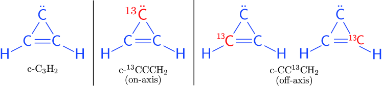
Figure 1: Molecular geometry of c-C₃H₂ and its ¹³C species

c-C₃H₂ is a carbon-chain related molecule, and is known to exist widely in interstellar clouds (e.g., Madden et al., 1989; Cox et al., 1989). It has two kinds of ¹³C isotopic species, as shown in Figure 1. The off-axis ¹³C species (referred to hereafter as c-$\mathrm{CC^{13}CH_{2}}$) is statistically favored by a factor of 2, because there are two equivalent carbon atoms in c-C₃H₂ for ¹³C substitution for this species. It was detected in TMC-1 and other sources (Madden et al., 1986; Gómez-González et al., 1986; Spezzano et al., 2013). On the other hand, detection of the on-axis ¹³C species (referred to hereafter as c-$\mathrm{{}^{13}CCCH_{2}}$) has not been reported in cold clouds as far as we know, although detection of one line was claimed by Gómez-González et al. (1986) toward the Galactic center cloud Sgr B2. During the spectral line surveys of L1527 with Nobeyama 45 m telescope (a legacy program of Nobeyama Radio Observatory) and IRAM 30 m telescope (the IRAM large program ASAI), we detected many spectral lines of the off-axis and on-axis ¹³C isotopic species as well as those of the main isotopologue. On the basis of these extensive datasets, we have explored the ¹³C abundance anomaly of c-C₃H₂ in L1527.

2 Observation

2.1 Observation with Nobeyama 45 m Telescope

The spectral line survey of the 3 mm band (80 GHz to 116 GHz) was carried out with Nobeyama 45 m telescope (referred to hereafter as NRO 45 m) toward L1527 from 2006 to 2011, as the legacy project of the Nobeyama Radio Observatory. Transition frequencies and quantum numbers of the observed lines for c-$\mathrm{C_{3}H_{2}}$ and its $\mathrm{{}^{13}C}$ species are listed in Tables 1–3. The observed position was $(\alpha_{2000},\ \delta_{2000})=(04^{\mathrm{h}}39^{\mathrm{m}}53\fs 89,\ 26\arcdeg 03\arcmin 11\farcs 0)$. In this observation, we used two SIS mixer receivers, S80 and S100, simultaneously in 2006–2008 and the dual-polarization sideband-separating SIS receiver T100H/V (Nakajima et al., 2008) in 2009–2011. The system temperatures varied from 250 to 350 K in 2006–2008 and from 150 to 250 K in 2009–2011. The pointing of the telescope was checked every $1\sim 1.5$ hours by observing nearby SiO maser sources (NML-Tau, Ori-KL), and was maintained to be better than 6″. The intensity scale was calibrated by the chopper-wheel method, and is estimated to be accurate within 20%. The main-beam efficiency is 0.43 in 2006–2008, 0.49 in 2009, 0.42 in 2010–2011, as reported in the NRO website. The beam size is 19″  at 86 GHz. In 2006–2011, we used a bank of acousto-optical radio spectrometers (AOSs) whose bandwidth, resolution, and channel spacing are 250 MHz, 250 kHz, and 125 kHz, respectively. In 2012, we used a bank of autocorrelators, SAM45, whose bandwidth, resolution, and channel spacing were set to be 500 MHz, 244 kHz, and 244 kHz, respectively. The frequency resolution corresponds to $\sim 0.8$ km s^-1 at 90 GHz. This resolution is not sufficient, because the typical line width toward this source is from $0.5$ to 0.8 km s^-1. However, we chose this resolution to cover the whole 3 mm band within the limited observation time. Although the lines are partly frequency-diluted, the integrated intensity is reliable. A position switching mode with the off-position, $(\alpha_{2000},\ \delta_{2000})=(04^{\mathrm{h}}42^{\mathrm{m}}35\fs 9,\ 25\arcdeg 53\arcmin 23\farcs 3)$, was employed in all the observations.

2.2 Observation with IRAM 30 m Telescope

Observations with IRAM 30 m telescope (referred to hereafter as IRAM 30 m) at Pico Veleta were performed in several runs between 2012 and 2013, as part of the ASAI (Astrochemical Surveys at IRAM) Large Program. The survey covers the spectral bands at 3 mm (80–112 GHz), 2 mm (130–173 GHz), and 1 mm (200–276 GHz). The beam size is 29″, 17″, and 12″  at 86, 145, and 210 GHz, respectively, as reported in the IRAM website. The wobbler switching mode was employed with a beam throw of 180″. This amount of the beam throw is enough, because most of the emission comes from the 15″–20″ diameter area around the protostar according to the interferometer observations combined with single-dish observations (Sakai et al., 2010b). The frontends were the broad-band EMIR receivers, and the backends were the FTS spectrometers in their 195 kHz resolution mode, corresponding to velocity resolutions of 0.21–0.73 km s^-1. The antenna temperature ($T_{\mathrm{A}}^{\ast}$) was converted to the main-beam brightness temperature ($T_{\mathrm{mb}}$) by dividing by $B_{\mathrm{eff}}/F_{\mathrm{eff}}$. Here, $B_{\mathrm{eff}}$ and $F_{\mathrm{eff}}$ are beam efficiency and forward efficiency, respectively. The $B_{\mathrm{eff}}/F_{\mathrm{eff}}$ value is 0.85, 0.80, and 0.67 at 86, 145, and 210 GHz, respectively.

3 Results

3.1 Overall results

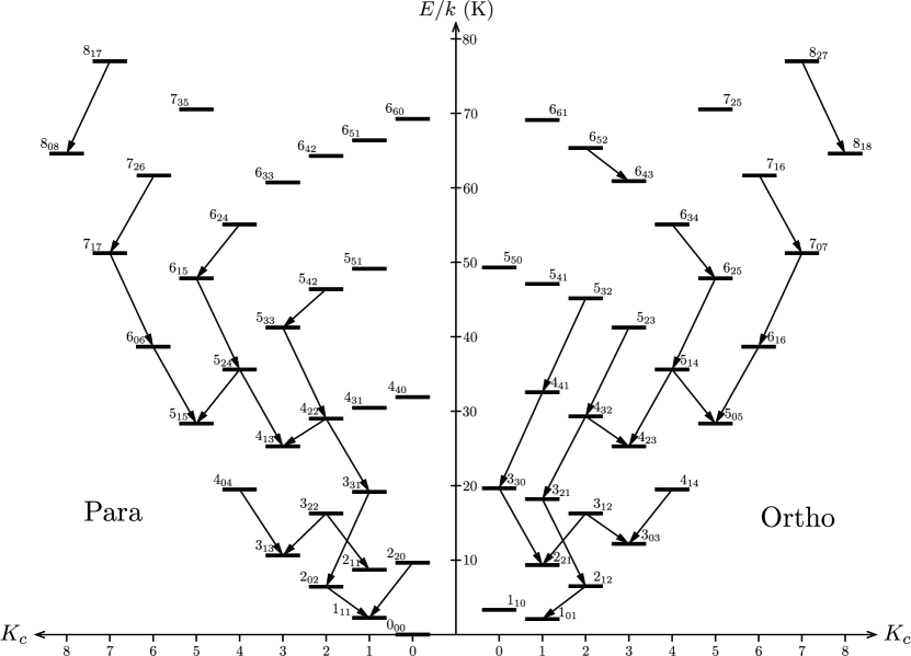
Figure 3: The energy level diagram of c-C₃H₂. The transitions observed in L1527 are shown by downward arrows.

In the Nobeyama observations, we detected 7 lines of c-C₃H₂ in the 3 mm band (Table 4). Later, we further detected 8, 9, and 17 lines in the 3 mm, 2 mm, and 1 mm bands in the ASAI observations. Examples of the observed spectra are shown in Figure 2, along with the best Gaussian fit to their profiles. In total, 41 lines of c-C₃H₂ were detected, among which 7 transitions were observed both in the Nobeyama and ASAI observations. Even high excitation lines of $8_{1,8}$–$8_{0,8}$ and $8_{2,7}$–$8_{1,8}$, whose upper state energies are as high as 77 K (53 cm^-1), were detected. The detected lines are summarized in Tables 1 and 4, and are also shown in the energy level diagram (Figure 3). Since c-C₃H₂ has a pair of equivalent H nuclei, the rotational levels are classified into the ortho and para species. Radiative and collisional interconversion between the ortho and the para species is strongly forbidden, and hence, the ortho and the para species behave as different molecular species. In our observations, 19 and 18 lines are detected for the ortho and para species, respectively, while the remaining 4 lines detected in the 1 mm band are blended lines of the ortho and para species.

In addition to the lines of normal species, we also detected the lines of the ¹³C isotopic species. The line parameters of c-$\mathrm{CC^{13}CH_{2}}$ and c-$\mathrm{{}^{13}CCCH_{2}}$ species (Figure 1) are summarized in Tables 2 and 3, respectively. For c-$\mathrm{CC^{13}CH_{2}}$, we detected 6 lines in the 3 mm band in the Nobeyama observations, and 2, 4, and 7 lines in the 3 mm, 2 mm, 1 mm bands, respectively, in the ASAI observations. In total, we detected 19 lines for c-$\mathrm{CC^{13}CH_{2}}$, as summarized in Tables 2 and 4. In contrast to the normal species, c-$\mathrm{CC^{13}CH_{2}}$ does not have the ortho and para classification, because the two hydrogen nuclei are no longer equivalent. For c-$\mathrm{{}^{13}CCCH_{2}}$, we detected 3 lines in the 3 mm band in the Nobeyama observations, and 2, 1, and 3 lines in the 3 mm, 2 mm, 1 mm bands, respectively, in the ASAI observations, as summarized in Tables 3 and 4. Hence, c-$\mathrm{{}^{13}CCCH_{2}}$ is definitively detected, as shown in Figure 2. This species has the ortho and para states as in the case of the normal species. It should be noted that c-$\mathrm{CC^{13}CH_{2}}$ is statistically favored by a factor of 2 in comparison with c-$\mathrm{{}^{13}CCCH_{2}}$, because two equivalent carbon atoms are available in c-C₃H₂ for ¹³C substitution for c-CC¹³CH₂ while only one for c-¹³CCCH₂ (Figure 1).

3.2 LTE analysis for c-C₃H₂

Assuming the local thermodynamic equilibrium (LTE) condition, we determine the rotation temperatures and the beam-averaged column densities of c-C₃H₂ and its ¹³C species by using the least-squares analysis with the following equations:

$$T_{\mathrm{b}}=\frac{h\nu}{k}\left[\frac{1}{\exp(h\nu/kT_{\mathrm{rot}})-1}-\frac{1}{\exp(h\nu/kT_{\mathrm{bg}})-1}\right](1-e^{-\tau}),$$

and

$$\tau=\frac{8\pi^{3}S\mu^{2}}{3h\Delta vU(T_{\mathrm{rot}})}\left[\exp\left(\frac{h\nu}{kT_{\mathrm{rot}}}\right)-1\right]\exp\left(-\frac{E_{\mathrm{u}}}{kT_{\mathrm{rot}}}\right)N,$$

where $T_{\mathrm{b}}$ is the brightness temperature, $h$ the Planck constant, $\nu$ the transition frequency, $k$ the Boltzmann constant, $T_{\mathrm{rot}}$ the rotation temperature, $T_{\mathrm{bg}}$ the cosmic microwave background temperature, $\tau$ the optical depth, $S$ the line strength, $\mu$ the dipole moment, $\Delta v$ the line width, $U(T_{\mathrm{rot}})$ the partition function, $E_{\mathrm{u}}$ the upper state energy, and $N$ the total column density. The partition function is numerically calculated from energies and degeneracies of the rotational levels, which are taken from the spectroscopy database, CDMS (Müller et al., 2005) (See also original spectroscopy references: Bogey et al. (1986); Vrtilek et al. (1987); Bogey et al. (1987); Spezzano et al. (2012).).

Because the size of the emitting region is comparable to or smaller than the telescope beam size, the effect of beam dilution has to be taken into account. This correction for the beam dilution is particularly important in this analysis, because the 1, 2 and 3 mm data, which result in different beam sizes, are used simultaneously. Furthermore, the correction is also necessary for the 3 mm data taken with the two different telescopes. The correction for the beam dilution is made by dividing the observed intensity by the beam dilution factor $\eta=\theta_{\mathrm{s}}^{2}/(\theta_{\mathrm{s}}^{2}+\theta_{\mathrm{b}}^{2}),$ where $\theta_{\mathrm{s}}$ and $\theta_{\mathrm{b}}$ denote the source diameter and the antenna beam width (FWHM), respectively. This correction factor assumes a Gaussian beam and a Gaussian distribution of the source emission. The FWHM beam widths are assumed to be $1.7\times 10^{3}/\nu$(GHz) and $2.4\times 10^{3}/\nu$(GHz) in arcseconds for NRO 45 m and IRAM 30 m, respectively, on the basis of the beam sizes mentioned in Sections 2.1 and 2.2. Sakai et al. (2010b) reported that c-$\mathrm{C_{3}H_{2}}$ is distributed within a diameter of 2000–3000 AU from the protostar, which corresponds to the size of 15″–20″. Thus, the size of the emitting region is assumed to be 20″. The intensities of the high excitation lines ($E_{\mathrm{u}}\gtrsim 30$ K) in the 3 mm band observed with NRO 45 m are brighter by a factor of 1.3–2.4 than those observed with IRAM 30 m, which further supports such a compact distribution. In the least-squares analysis, the ortho and para species are treated as different molecules, and the ortho-to-para ratio is taken as a fitting parameter. This analysis is possible owing to the large dataset of the observed line intensities. Relative weights of the data are determined by the errors of the line parameters including the uncertainty of the intensity calibration (20%). The total (ortho plus para) column density is derived to be $(1.08\pm 0.16)\times 10^{14}$ cm^-2. The ortho-to-para ratio is evaluated to be $3.1\pm 0.4$, which is comparable to the statistical weight of 3. This ratio is consistent with the previous report by Takakuwa et al. (2001) ($2.5\pm 0.5$). The rotation temperature is ($8.3\pm 0.3$) K, which is lower than that reported for C₄H₂ in L1527 of 12.3 K (Sakai et al., 2008). The errors denote the standard deviation of the fit.

We also estimated the column densities of the two ¹³C species, c-$\mathrm{{}^{13}CCCH_{2}}$ and c-$\mathrm{CC^{13}CH_{2}}$, by assuming LTE condition. The column density and the rotation temperature of c-$\mathrm{{}^{13}CCCH_{2}}$ are evaluated to be $(3.5\pm 0.7)\times 10^{11}$ cm^-2 and $(8.6\pm 1.5)$ K, respectively, by assuming the same ortho-to-para ratio as the normal species. On the other hand, the column density and the excitation temperature of c-$\mathrm{CC^{13}CH_{2}}$ are determined to be $(1.79\pm 0.19)\times 10^{12}$ cm^-2 and $(7.3\pm 0.4)$ K, respectively. The abundance ratio of [c-C₃H₂]/[c-$\mathrm{{}^{13}CCCH_{2}}$] is thus determined to be $310\pm 80$, whereas that of [c-C₃H₂]/[c-$\mathrm{CC^{13}CH_{2}}$] is $61\pm 11$. [c-$\mathrm{CC^{13}CH_{2}}$] represents the total abundance of the c-$\mathrm{CC^{13}CH_{2}}$ species without any correction for the statistical factor of 2 (Figure 1; Section 3.1). These results are higher than the ratios expected for the condition that ¹³C is randomly distributed among the three carbon atoms and the elemental abundance ratio of ¹²C/¹³C is 60–70, as shown in Table 5.

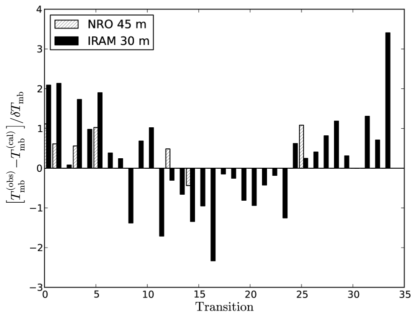
Figure 4: Residuals of the LTE fit divided by uncertainty of each line, arranged in ascending order of the upper-state energy.

Figure 4 shows the residuals in the least-squares fit divided by the uncertainty $\delta T$ of each line, $(T_{\mathrm{obs}}-T_{\mathrm{fit}})/\delta T$, where $T_{\mathrm{obs}}$ and $T_{\mathrm{fit}}$ are the observed intensity and the best-fit value, respectively. The uncertainty of the intensity $\delta T$ for each line is estimated by taking into account the Gaussian fitting error of the line profile and the calibration uncertainty. Figure 4 shows a slight systematic residuals in the fit. Intensities of the lines with high and low upper state energies systematically show positive residuals, while those of the lines with moderate upper state energies tend to have negative residuals. Such a systematic trend can also be seen, even if the different source sizes of 15″ and 30″ are assumed. This may indicate that the source includes two components having different rotation temperatures. The physical structure of the source (i.e. the gradient in the density and the temperature) may also play a role. However, the systematic residuals are eliminated by a non-LTE analysis described below, and we therefore consider that the systematic residuals mainly originate from imperfection of the LTE assumption.

3.3 LVG analysis for c-C₃H₂

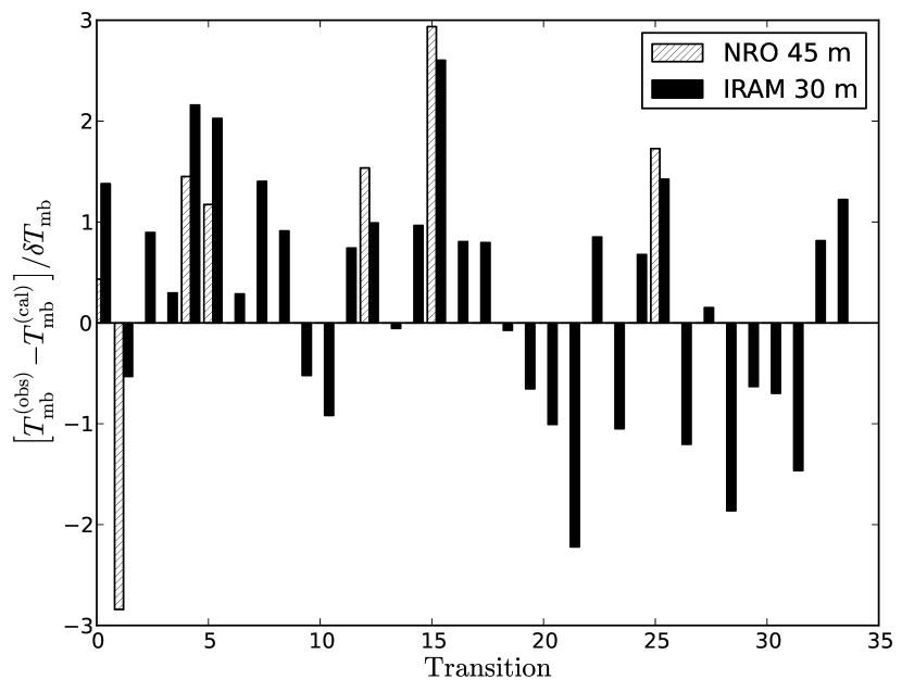
Figure 5: The same as Figure 4, but obtained by assuming the LVG condition.

We employ a large velocity gradient (LVG) analysis based on the non-LTE radiative transfer code Radex (van der Tak et al., 2007) for the analysis of the normal species. If the gas kinetic temperature is assumed to be 25 K (Sakai et al., 2010b), the H₂ density and the total column density of c-C₃H₂ are determined to be $(2.9\pm 0.5)\times 10^{5}$ cm^-3 and $(8.8\pm 1.1)\times 10^{13}$ cm^-2, respectively. Even if the gas kinetic temperature is assumed to be 10 K for reference, the total column density of c-C₃H₂ does not change very much ($(1.18\pm 0.11)\times 10^{14}$ cm^-2). Figure 5 shows the residuals of the fit for the gas kinetic temperature of 25 K, calculated in the same way as in Figure 4. The systematic errors seen in Figure 4 are now eliminated in Figure 5. Although the non-LTE analysis is favorable as seen here, the collisional cross sections are not reported for the ¹³C isotopic species. Hence, we cannot determine the abundance ratios of the ¹³C isotopic species relative to the normal species by using the non-LTE analysis. Since the total column density derived from the non-LTE analysis only differs from that derived from the LTE analysis by 20%, we employ the LTE results for discussions of the ¹²C/¹³C ratio of c-C₃H₂.

4 Discussion

4.1 Dilution of the ¹³C species

The ¹²C/¹³C ratios of c-C₃H₂ derived from the column densities are summarized in Table 5. The averaged ¹²C/¹³C ratio of c-C₃H₂ is calculated as

$$R_{\mathrm{av}}=\frac{3[\mathrm{c\mathchar 45\relax C_{3}H_{2}}]}{[\mathrm{c\mathchar 45\relax^{13}CCCH_{2}}]+[\mathrm{c\mathchar 45\relax CC^{13}CH_{2}}]}.$$ (1)

The numerical factor 3 is introduced because three carbon atoms are available for the ¹³C substitution. The $R_{\mathrm{av}}$ values are evaluated to be $150\pm 30$ under the LTE condition. As shown in Table 5, the ¹²C/¹³C ratios of c-C₃H₂ are thus found to be higher than those expected from the interstellar elemental abundance ratio of 60–70 (Lucas & Liszt, 1998; Milam et al., 2005). For comparison, we have also derived the ¹²C/¹³C ratio in L1527 by using the $J=1$–$0$ line data of C¹⁸O and ¹³C¹⁸O obtained in the ASAI and Nobeyama observations to be $68\pm 19$. The $R_{\mathrm{av}}$ value obtained above is also higher than this ratio.

In dense molecular clouds, the main reservoir of ¹³C is ¹³CO, which is the most abundant carbon-bearing molecule. As carbon-chain molecules are produced by reactions starting from C⁺, their ¹³C species are formed by the reaction from ¹³C⁺. Although the ¹³C⁺ ion is produced from ¹³CO with the reactions of He⁺, as ¹²C⁺ from ¹²CO, ¹³C⁺ will go back to ¹³CO by the following isotope exchange reaction (Langer et al., 1984; Roueff et al., 2015):

$$\mathrm{{}^{13}C^{+}+{}^{12}CO\rightarrow{}^{13}CO+{}^{12}C^{+}+35\ K.}$$ (2)

This is the most important reaction for ¹³C⁺, because the reaction with H₂ is a very slow radiative association. The electron recombination is also much slower than the reaction with ¹²CO. This exchange reaction is exothermic, and hence, its backward reaction is slow in cold clouds. Then, the ¹²C⁺/¹³C⁺ ratio tends to be higher in cold clouds. The ¹³C species of various molecules produced from ¹³C⁺ thus become less abundant. This mechanism was initially proposed by Langer et al. (1984). Woods & Willacy (2009) and Furuya et al. (2011) confirmed this trend by chemical model calculations. It should be noted that the isotope selective photodissociation, which could cause the ¹²C/¹³C isotope anomaly in photodissociation regions, is not important in our observations, because we are observing a dense part near the protostar.

Such a dilution process can occur even in the protostellar envelope of L1527, whose gas kinetic temperature is 25 K (Sakai et al., 2010b, 2014). In order to verify this, we consider the following relation under the steady-state approximation:

$$\frac{[\mathrm{{}^{13}C^{+}}]}{[\mathrm{{}^{12}C^{+}}]}=\frac{k_{\mathrm{b}}[\mathrm{{}^{13}CO}]}{k_{\mathrm{f}}[\mathrm{{}^{12}CO}]},$$ (3)

where $k_{\mathrm{f}}$ and $k_{\mathrm{b}}$ are the rate coefficients of the forward and backward reactions of (2), respectively, and $[X]$ denotes the abundance of $X$. These rate coefficients fulfill the following relation:

$$k_{\mathrm{b}}=k_{\mathrm{f}}\exp\left(-\frac{\Delta G}{kT}\right),$$ (4)

where $\Delta G$ represents the free energy difference between the right and left hand sides of the reaction (2). Since $k_{\mathrm{b}}/k_{\mathrm{f}}$ is evaluated to be 0.2 at 25 K, the dilution process of ¹³C⁺ is barely possible in the warm region of L1527.

L1527 is a warm-carbon-chain-chemistry source, where CH₄ evaporated from dust grains in the warm ($\gtrsim 25$ K) and the dense part near the protostar triggers efficient production of carbon-chain molecules including c-C₃H₂. CH₄ is thought to be formed by hydrogenation from the neutral carbon atoms depleted onto dust grains in the cold starless core phase and/or the less dense phase. The ¹²C/¹³C ratio of the carbon atom is also expected to be larger than the elemental ratio as the ¹²C⁺/¹³C⁺ ratio, because the neutral carbon atom (C) is formed from electron recombination of the carbon ion (C⁺). Hence, the ¹²C/¹³C ratio of CH₄ formed on dust grains would also be higher. This may also contribute to the dilution of the ¹³C species of c-C₃H₂.

4.2 Abundance difference between two ¹³C species

As described in the Introduction, it is reported that several carbon-chain molecules show the abundance anomaly of the ¹³C species. For CCH, CCS, C₃S, C₄H, and HC₃N, the ¹³C abundances for different carbon atoms in a single molecular species are different from one another. In order to compare the abundance of the two ¹³C species (Section 3.1), we calculate the $[\mathrm{c\mathchar 45\relax^{13}CCCH_{2}}]/[\mathrm{c\mathchar 45\relax CC^{13}CH_{2}}]$ ratio to be $0.20\pm 0.05$. If ¹³C were randomly substituted for the three carbon atoms, the [c-$\mathrm{{}^{13}CCCH_{2}}$]/[c-$\mathrm{CC^{13}CH_{2}}$] ratio would be 0.5. Hence, the observed ratio indicates that c-$\mathrm{CC^{13}CH_{2}}$ exists more favorably than c-$\mathrm{{}^{13}CCCH_{2}}$. It has been thought that the main production pathway for c-C₃H₂ is the electron recombination of $\mathrm{C_{3}H_{3}^{+}}$. This is because the cyclopropenyl cation $\mathrm{C_{3}H_{3}^{+}}$ is a major ionic species, which is produced by the gas-phase reactions starting from CH₄ (Sakai & Yamamoto, 2013). Since $\mathrm{C_{3}H_{3}^{+}}$ has three equivalent carbon atoms, c-C₃H₂ produced from $\mathrm{C_{3}H_{3}^{+}}$ cannot contribute to the abundance anomaly of ¹³C species. Hence, other reactions have to be considered as the dominant production pathway (e.g., $\mathrm{C_{2}H_{2}+CH\rightarrow C_{3}H_{2}+H}$).

Another possible reason for the abundance anomaly of the two ¹³C species is the exchange reaction between c-$\mathrm{{}^{13}CCCH_{2}}$ and c-$\mathrm{CC^{13}CH_{2}}$, although it is uncertain whether this reaction happens for the closed shell molecule, c-C₃H₂. The zero-point vibrational energies of c-$\mathrm{{}^{13}CCCH_{2}}$ and c-$\mathrm{CC^{13}CH_{2}}$ are evaluated to be lower than the normal species by 8.74 K and 53.2 K, respectively, by using the molecular constants by Dateo & Lee (1997). Hence, it would be possible that c-$\mathrm{CC^{13}CH_{2}}$ is enhanced relative to c-$\mathrm{{}^{13}CCCH_{2}}$, if the exchange reaction is possible. In case of ¹³CCH and C¹³CH, the reaction such as

$$\mathrm{{}^{13}CCH+H\rightarrow C{}^{13}CH+H}$$ (5)

is proposed (Sakai et al., 2010a). It is thus interesting to explore whether a similar process is possible for c-C₃H₂. It should be noted that the isotopologue with the lowest zero-point vibrational energy tends to have higher abundances for CCH, CCS, and C₃S, although this trend is uncertain for C₄H (Sakai et al., 2007, 2010a, 2013). This fact may suggest possible contribution of the position exchange reactions (Sakai et al., 2010a; Furuya et al., 2011). More detailed studies of these reactions as well as chemical model calculations for the ¹³C species in molecular clouds are awaited.

5 Concluding Remarks

In this study, we accurately determined the [c-C₃H₂]/[c-$\mathrm{{}^{13}CCCH_{2}}$] and [c-C₃H₂]/[c-$\mathrm{CC^{13}CH_{2}}$] ratios on the basis of the extensive data of the Nobeyama and ASAI observations. We found a significant dilution of the ¹³C species, and a significant difference between the [c-C₃H₂]/[c-$\mathrm{{}^{13}CCCH_{2}}$] and [c-C₃H₂]/[c-$\mathrm{CC^{13}CH_{2}}$] ratios, even when the statistical factor of 2 for the c-$\mathrm{CC^{13}CH_{2}}$ species is taken into account. This further confirms that the ¹³C anomaly is an important phenomenon in astrochemistry.

It should be noted that determination of the ¹²C/¹³C ratio requires accurate determination of the column density of the normal species. This was indeed possible in this study, where a large number of lines can be used to conduct a fine analysis. However, this is not always the case. On the other hand, the anomaly in the ¹²C/¹³C ratio among the different carbon atoms in a single molecule can be studied only by observations of the ¹³C species, which often emit optically thin lines. If the cause of the ¹²C/¹³C anomaly in a single molecule is established, it could be a new tracer to understand chemical processes and physical conditions of molecular clouds.

The anomalies of the ¹³C species found for c-C₃H₂ and other carbon-chain molecules might be related to the ¹³C anomaly in meteorites (Floss et al., 2006). Although the ¹²C/¹³C anomaly in dust forming regions of AGB stars (e.g., Milam et al., 2009; Kahane et al., 1992; Tomkin et al., 1976) mainly contributes to the anomaly in meteorites, the ¹²C/¹³C anomaly in cold molecular clouds may also be responsible. Hence, understanding the abundance anomaly of the ¹³C species and its evolution in star-forming regions is of particular importance to trace back from our planetary system to its interstellar origins.

Figure 2: Observed line profiles of c-C₃H₂ and its ¹³C species in L1527. The results of Gaussian fitting are also shown in red.

Table 1: Observed line parameters of c-C₃H₂ toward L1527

Frequency	Transition	o/p	$E_{\mathrm{u}}$	$\langle S\mu^{2}\rangle$	$\Delta V_{\mathrm{LSR}}$	$\Delta v$	rms	$T_{\mathrm{mb}}$	$\int T_{\mathrm{mb}}dv$	$\sigma_{\mathrm{LTE}}$	$\sigma_{\mathrm{LVG}}$	telescope
(GHz)			(K)	(Debye2)	(km s-1)	(km s-1)	(mK)	(K)	(K km s-1)
80.723180	$4_{2,2}$–$4_{1,3}$	p	28.8	19.5	$-0.07(4)$	1.72(9)	5.8	0.12(3)	$0.25(5)$	$0.48$	$1.54$	NRO
					$-0.09(6)$	0.81(10)	5.9	0.14(3)	$0.11(2)$	$-0.30$	$0.99$	IRAM
82.093544	$2_{0,2}$–$1_{1,1}$	p	6.4	14.6	$-0.15(13)$	1.40(3)	34.3	1.5(3)	$2.5(5)$	$1.11$	$0.43$	NRO
					$-0.030(4)$	0.820(11)	3.9	1.8(4)	$1.6(3)$	$2.09$	$1.38$	IRAM
82.966200	$3_{1,2}$–$3_{0,3}$	o	16.0	31.3	$-0.101(7)$	1.255(17)	15.2	1.1(2)	$1.6(3)$	$0.56$	$1.45$	NRO
					$-0.063(4)$	0.788(5)	3.5	1.4(3)	$1.2(2)$	$1.73$	$2.16$	IRAM
84.727688	$3_{2,2}$–$3_{1,3}$	p	16.1	10.3	$0.150(5)$	1.154(12)	5.5	0.52(11)	$0.67(13)$	$1.02$	$1.17$	NRO
					$-0.037(5)$	1.196(10)	2.7	0.42(8)	$0.54(11)$	$1.90$	$2.03$	IRAM
85.338894	$2_{1,2}$–$1_{0,1}$	o	6.4	48.1	$0.340(6)$	1.239(14)	21.1	2.8(6)	$3.8(8)$	$0.61$	$-2.84$	NRO
					$-0.070(5)$	1.065(16)	2.9	2.8(6)	$3.3(7)$	$2.14$	$-0.53$	IRAM
85.656431	$4_{3,2}$–$4_{2,3}$	o	29.1	56.2	$-0.010(9)$	1.16(2)	7.4	0.46(9)	$0.57(11)$	$-0.44$	$2.94$	NRO
					$-0.060(9)$	1.15(3)	2.1	0.26(5)	$0.33(7)$	$-1.34$	$2.60$	IRAM
87.435318	$5_{4,2}$–$5_{3,3}$	p	45.3	26.2	$-0.2(2)$	2.0(5)	10.5	0.032(9)	$0.045(19)$	$1.08$	$1.73$	NRO
					$0.00(11)$	1.9(3)	1.8	0.016(4)	$0.036(8)$	$0.25$	$1.42$	IRAM
90.344082	$6_{5,2}$–$6_{4,3}$	o	64.7	98.3	$-0.16(19)$	1.2(5)	3.8	0.014(5)	$0.017(7)$	$0.71$	$0.81$	IRAM
145.089606	$3_{1,2}$–$2_{2,1}$	o	16.0	40.0	$0.004(2)$	0.727(5)	12.8	3.0(6)	$2.3(5)$	$0.98$	$0.30$	IRAM
150.436555	$2_{2,0}$–$1_{1,1}$	p	9.7	6.8	$-0.136(2)$	0.634(8)	8.8	1.7(3)	$1.2(2)$	$0.080$	$0.89$	IRAM
150.820665	$4_{0,4}$–$3_{1,3}$	p	19.3	36.9	$-0.162(4)$	0.779(10)	8.2	2.3(5)	$1.9(4)$	$0.68$	$-0.52$	IRAM
150.851908	$4_{1,4}$–$3_{0,3}$	o	19.3	110.7	$-0.201(13)$	0.92(3)	8.3	3.3(7)	$3.2(6)$	$1.02$	$-0.92$	IRAM
150.954691	$6_{2,4}$–$6_{1,5}$	p	54.7	20.3	$-0.23(8)$	0.6(3)	9.3	0.05(2)	$0.025(9)$	$0.31$	$-0.63$	IRAM
151.039173	$6_{3,4}$–$6_{2,5}$	o	54.7	60.8	$-0.10(4)$	0.71(9)	8.8	0.10(2)	$0.085(20)$	$-0.010$	$-0.70$	IRAM
151.343878	$5_{1,4}$–$5_{0,5}$	o	35.4	32.4	$-0.065(8)$	0.811(17)	6.7	0.43(9)	$0.37(8)$	$-0.15$	$0.79$	IRAM
151.361105	$5_{2,4}$–$5_{1,5}$	p	35.4	10.8	$0.00(2)$	0.75(5)	6.4	0.14(3)	$0.11(2)$	$-0.94$	$-0.65$	IRAM
155.518303	$3_{2,2}$–$2_{1,1}$	p	16.1	17.8	$0.005(2)$	0.687(5)	8.2	2.0(4)	$1.5(3)$	$0.38$	$0.29$	IRAM
204.788926	$4_{2,2}$–$3_{3,1}$	p	28.8	11.2	$-0.036(7)$	0.761(16)	7.4	0.52(10)	$0.44(9)$	$-0.66$	$-0.054$	IRAM
216.278756	$3_{3,0}$–$2_{2,1}$	o	19.5	45.6	$-0.128(7)$	0.892(15)	5.2	2.0(4)	$1.9(4)$	$-1.71$	$0.74$	IRAM
217.822148	$6_{0,6}$–$5_{1,5}$, $6_{1,6}$–$5_{0,5}$	p/o	38.6	58.3	$-0.092(3)$	0.922(8)	4.4	2.5(5)	$2.5(5)$	$-0.42$	$-2.22$	IRAM
217.940046	$5_{1,4}$–$4_{2,3}$	o	35.4	110.3	$-0.057(2)$	0.863(5)	5.5	1.8(4)	$1.7(3)$	$-0.25$	$-0.073$	IRAM
218.160456	$5_{2,4}$–$4_{1,3}$	p	35.4	36.8	$-0.022(4)$	0.815(11)	6.5	0.73(15)	$0.63(13)$	$-0.81$	$-1.01$	IRAM
218.732732	$7_{2,6}$–$7_{1,7}$, $7_{1,6}$–$7_{0,7}$	p/o	61.2	11.0	$0.05(3)$	0.92(8)	4.4	0.071(15)	$0.084(18)$	$1.31$	$-1.46$	IRAM
227.169138	$4_{3,2}$–$3_{2,1}$	o	29.1	61.6	$-0.093(4)$	0.827(9)	8.4	1.8(4)	$1.6(3)$	$-0.95$	$0.96$	IRAM
244.222150	$3_{2,1}$–$2_{1,2}$	o	18.2	7.3	$-0.047(3)$	0.761(6)	6.0	1.5(3)	$1.2(2)$	$0.24$	$1.40$	IRAM
249.054368	$5_{2,3}$–$4_{3,2}$	o	41.0	76.3	$-0.050(4)$	0.791(10)	5.1	1.0(2)	$0.89(18)$	$-0.18$	$0.85$	IRAM
251.314367	$7_{1,7}$–$6_{0,6}$, $7_{0,7}$–$6_{1,6}$	p/o	50.7	69.0	$-0.014(3)$	0.830(8)	5.7	1.6(3)	$1.5(3)$	$1.19$	$-1.86$	IRAM
251.508709	$6_{1,5}$–$5_{2,4}$	p	47.5	47.4	$0.029(9)$	0.74(2)	6.0	0.41(8)	$0.35(7)$	$0.41$	$-1.20$	IRAM
251.527311	$6_{2,5}$–$5_{1,4}$	o	47.5	142.2	$-0.005(4)$	0.791(10)	6.4	1.1(2)	$1.0(2)$	$0.81$	$0.15$	IRAM
252.409837	$8_{1,7}$–$8_{0,8}$, $8_{2,7}$–$8_{1,8}$	p/o	76.5	11.1	$-0.05(6)$	0.94(14)	5.3	0.051(12)	$0.038(10)$	$3.41$	$1.22$	IRAM
254.987652	$5_{3,3}$–$4_{2,2}$	p	41.1	26.8	$0.048(8)$	0.752(18)	5.6	0.36(7)	$0.30(6)$	$-1.25$	$-1.04$	IRAM
260.479746	$5_{3,2}$–$4_{4,1}$	o	44.7	25.8	$0.00(11)$	0.83(3)	6.8	0.32(6)	$0.31(6)$	$0.62$	$0.68$	IRAM
261.831811	$3_{3,1}$–$2_{0,2}$	p	19.0	1.4	$0.02(3)$	0.68(6)	18.4	0.30(6)	$0.19(4)$	$-1.38$	$0.91$	IRAM
265.759481	$4_{4,1}$–$3_{3,0}$	o	32.2	89.8	$-0.076(5)$	0.879(13)	8.2	1.4(3)	$1.4(3)$	$-2.33$	$0.80$	IRAM

Note. — The numbers in parentheses represent the errors in unit of last significant digits.

Table 2: Observed line parameters of c-CC¹³CH₂ toward L1527

Frequency	Transition	$E_{\mathrm{u}}$	$\langle S\mu^{2}\rangle$	$\Delta V_{\mathrm{LSR}}$	$\Delta v$	rms	$T_{\mathrm{mb}}$	$\int T_{\mathrm{mb}}dv$	$\sigma_{\mathrm{LTE}}$	telescope
(GHz)		(K)	(Debye2)	(km s-1)	(km s-1)	(mK)	(K)	(K km s-1)
80.047537	$2_{0,2}$–$1_{1,1}$	6.3	27.8	$-0.07(2)$	1.25(5)	7.5	0.16(3)	$0.23(5)$	$1.68$	NRO
80.775347	$3_{1,2}$–$3_{0,3}$	15.7	21.0	$0.19(16)$	1.5(4)	6.4	0.021(6)	$0.036(11)$	$0.29$	NRO
83.474137	$3_{2,2}$–$3_{1,3}$	15.9	20.5	$-0.00(16)$	1.5(4)	6.8	0.022(7)	$0.033(12)$	$0.35$	NRO
				$0.00(2)$	1.1(5)	3.5	0.018(5)	$0.027(7)$	$0.053$	IRAM
84.185635	$2_{1,2}$–$1_{0,1}$	6.3	31.3	$0.015(10)$	1.18(2)	4.3	0.21(4)	$0.28(6)$	$1.65$	NRO
				$-0.08(2)$	0.78(5)	3.6	0.26(5)	$0.22(4)$	$2.29$	IRAM
114.897371	$3_{0,3}$–$2_{1,2}$	11.8	50.5	$0.00(4)$	0.90(6)	19.6	0.32(7)	$0.30(6)$	$0.80$	NRO
115.524356	$3_{1,3}$–$2_{0,2}$	11.8	50.7	$-0.00(6)$	0.78(7)	22.3	0.31(7)	$0.32(7)$	$-0.052$	NRO
140.432881	$3_{1,2}$–$2_{2,1}$	15.7	23.9	$-0.13(3)$	0.53(10)	7.3	0.15(4)	$0.081(18)$	$0.25$	IRAM
147.702239	$2_{2,0}$–$1_{1,1}$	9.6	13.9	$-0.18(3)$	0.65(5)	9.4	0.17(4)	$0.10(2)$	$0.021$	IRAM
148.114191	$4_{1,4}$–$3_{0,3}$	19.0	71.6	$-0.161(18)$	0.78(4)	6.9	0.18(4)	$0.14(3)$	$-0.40$	IRAM
153.894626	$3_{2,2}$–$2_{1,1}$	15.9	34.8	$-0.10(2)$	0.63(6)	9.2	0.16(4)	$0.13(3)$	$-0.83$	IRAM
212.457672	$3_{3,0}$–$2_{2,1}$	19.2	31.7	$-0.02(5)$	0.94(11)	7.3	0.081(18)	$0.083(19)$	$-3.06$	IRAM
213.843018	$6_{1,6}$–$5_{0,5}$, $6_{0,6}$–$5_{1,5}$	37.9	113.5	$0.02(3)$	0.96(6)	4.4	0.088(18)	$0.085(18)$	$0.66$	IRAM
213.872779	$5_{1,4}$–$4_{2,3}$	34.8	70.7	$0.06(5)$	0.79(11)	4.4	0.045(10)	$0.029(7)$	$0.11$	IRAM
214.313034	$5_{2,4}$–$4_{1,3}$	34.8	70.8	$-0.07(5)$	0.82(11)	4.2	0.052(12)	$0.060(13)$	$0.78$	IRAM
225.435934	$4_{3,2}$–$3_{2,1}$	28.6	40.3	$0.02(9)$	1.00(2)	7.9	0.051(14)	$0.044(14)$	$-0.027$	IRAM
237.998109	$3_{2,1}$–$2_{1,2}$	17.8	5.1	$-0.08(6)$	0.71(14)	4.3	0.037(10)	$0.019(6)$	$-0.53$	IRAM
246.723236	$7_{1,7}$–$6_{0,6}$, $7_{0,7}$–$6_{1,6}$	49.7	134.3	$0.21(6)$	0.70(14)	5.6	0.044(12)	$0.040(10)$	$1.25$	IRAM

Note. — The numbers in parentheses represent the errors in unit of last significant digits.

Table 3: Observed line parameters of c-¹³CCCH₂ toward L1527

Frequency	Transition	o/p	$E_{\mathrm{u}}$	$\langle S\mu^{2}\rangle$	$\Delta V_{\mathrm{LSR}}$	$\Delta v$	rms	$T_{\mathrm{mb}}$	$\int T_{\mathrm{mb}}dv$	$\sigma_{\mathrm{LTE}}$	telescope
(GHz)			(K)	(Debye2)	(km s-1)	(km s-1)	(mK)	(K)	(K km s-1)
81.150881	$2_{0,2}$–$1_{1,1}$	p	6.3	31.0	$0.10(18)$	1.3(4)	5.5	0.016(5)	$0.021(8)$	$0.84$	NRO
					$-0.00(3)$	0.9(3)	4.1	0.018(6)	$0.026(8)$	$1.17$	IRAM
82.303747	$2_{1,2}$–$1_{0,1}$	o	6.3	96.2	$-0.17(12)$	1.1(3)	12.6	0.048(14)	$0.049(16)$	$0.22$	NRO
					$-0.08(7)$	0.83(8)	3.9	0.064(14)	$0.060(13)$	$2.07$	IRAM
114.381212	$3_{0,3}$–$2_{1,2}$	o	11.8	159.0	$-0.15(11)$	1.1(2)	14.8	0.08(2)	$0.07(3)$	$0.30$	NRO
145.353129	$3_{1,2}$–$2_{2,1}$	o	15.7	96.1	$0.10(11)$	0.6(2)	10.3	0.044(16)	$0.033(13)$	$-0.80$	IRAM
211.613800	$3_{3,0}$–$2_{2,1}$	o	18.9	75.0	$0.02(7)$	0.69(17)	4.9	0.033(10)	$0.024(7)$	$-2.15$	IRAM
212.387110	$6_{0,6}$–$5_{1,5}$, $6_{1,6}$–$5_{0,5}$	p/o	37.6	117.2	$0.18(9)$	0.8(2)	6.5	0.039(12)	$0.026(8)$	$0.39$	IRAM
245.044421	$7_{1,7}$–$6_{0,6}$, $7_{0,7}$–$6_{1,6}$	p/o	49.4	138.6	$-0.04(10)$	1.2(2)	4.8	0.029(8)	$0.033(10)$	$2.72$	IRAM

Note. — The numbers in parentheses represent the errors in unit of last significant digits.

Table 4: Number of detected lines.

	NRO 45 m	IRAM 30 m
Species	3 mm	3 mm	2 mm	1 mm	Total
c-C3H2	7	8	9	17	41
c-CC13CH2	6	2	4	7	19
c-13CCCH2	3	2	1	3	9

Table 5: The observed ¹²C/¹³C ratios of c-C₃H₂.

Ratio	Observed	Expected
$\mathrm{[}$c-C3H${}_{2}\mathrm{]/[}$c-CC13CH2]	$61\pm 11$	30–35
$\mathrm{[}$c-C3H${}_{2}\mathrm{]/[}$c-13CCCH2]	$310\pm 80$	60–70
3[c-C3H${}_{2}\mathrm{]/([}$c-CC13CH2]+[c-13CCCH2])	$150\pm 30$	60–70
$\mathrm{[}$c-13CCCH${}_{2}\mathrm{]/[}$c-CC13CH2]	$0.20\pm 0.05$	0.5

References

- Bogey et al. (1986) Bogey, M., Demuynck, C., & Destombes, J. L. 1986, Chem. Phys. Lett., 125, 383
- Bogey et al. (1987) Bogey, M., Demuynck, C., Destombes, J. L., & Dubus, H. 1987, J. Mol. Spectrosc., 122, 313
- Cox et al. (1989) Cox, P., Walmsley, C. M., & Güsten, R. 1989, A&A, 209, 382
- Dateo & Lee (1997) Dateo, C. E., & Lee, T. J. 1997, Spectrochim. Acta, A53, 1065.
- Floss et al. (2006) Floss, C., Stadermann, F. J., Bradley, J. P., Dai, Z. R., Bajt, S., Graham, G., & Lea, A. S. 2006, Geochim. Cosmochim. Acta, 70, 2371
- Furuya et al. (2011) Furuya, K., Aikawa, Y., Sakai, N., & Yamamoto, S. 2011, ApJ, 731, 38
- Gómez-González et al. (1986) Gómez-González, J., Guélin, M., Cernicharo, J., Kahane, C., & Bogey, M. 1986, A&A, 168, L11
- Kahane et al. (1992) Kahane, C., Cernicharo, J., Gómez-González, J., & Guélin, M. 1992, A&A, 256, 235
- Langer et al. (1984) Langer, W. D., Graedel, T. E., Frerking, M. A., & Armentrout, P. B. 1984, ApJ, 277, 581
- Liszt & Ziurys (2012) Liszt, H. S. & Ziurys, L. M. 2012, ApJ, 747, 55
- Lucas & Liszt (1998) Lucas, R., & Liszt, H. 1998, A&A, 337, 246
- Madden et al. (1986) Madden, S. C., Irvine, W. M., & Matthews, H. E. 1986, ApJ, 311, L27
- Madden et al. (1989) Madden, S. C., Irvine, W. M., Matthews, H. E., Friberg, P., & Swade D. A. 1989, AJ, 97, 1403
- Milam et al. (2005) Milam, S. N., Savage, C., Brewster, M. A., Ziurys, L. M., & Wyckoff, S. 2005, ApJ, 634, 1126
- Milam et al. (2009) Milam, S. N., Woolf, N. J., & Ziurys, L. M. 2009, ApJ, 690, 837
- Müller et al. (2005) Müller, H. S. P., Schlöder, F., Stutzki, J., & Winnewisser, G. 2005, JMoSt, 742, 215
- Nakajima et al. (2008) Nakajima, T., Sakai, T., Asayama, S., et al. 2008, PASJ, 60, 435
- Roueff et al. (2015) Roueff, E., Loison, J. C., & Hickson, K. M. 2015, arXiv: 1501.01141v2
- Sakai et al. (2007) Sakai, N., Ikeda, M., Morita, M., Sakai, T., Takano, S., Osamura, Y., & Yamamoto, S. 2007, ApJ, 663, 1174
- Sakai et al. (2008) Sakai, N., Sakai, T., Hitora, T., & Yamamoto, S. 2008, ApJ, 672, 371
- Sakai et al. (2010a) Sakai, N., Saruwatari, O., Sakai, T., Takano, S., & Yamamoto, S. 2010a, A&A, 512, A31
- Sakai et al. (2010b) Sakai, N., Sakai, T., Hitora, T., & Yamamoto, S. 2010b, ApJ, 722, 1633
- Sakai et al. (2014) Sakai, N., Sakai, T., Hirota, T., et al. 2014, Nature, 507, 78
- Sakai et al. (2013) Sakai, N., Takano, S., Sakai, T., Shiba, S., Sumiyoshi, S., Endo, Y., & Yamamoto, S. 2013, JPC, 117, 9831
- Sakai & Yamamoto (2013) Sakai, N. & Yamamoto, S. 2013, ChRv, 113, 8981
- Spezzano et al. (2012) Spezzano, S., Tamassia, F., Thorwirth, S., Thaddeus, P., Gottlieb, C. A., & McCarthy, M. C. 2012, ApJS, 200, 1
- Spezzano et al. (2013) Spezzano, S., Brünken, S., Schilke, P., et al. 2013, ApJ, 769, L19
- Takakuwa et al. (2001) Takakuwa, S., Kawaguchi, K., Mikami, H., & Saito, M. 2001, PASJ, 53, 251
- Takano et al. (1998) Takano, S., Masuda, A., Hirahara, Y., et al. 1998, A&A, 329, 1156
- Tomkin et al. (1976) Tomkin, J., Luck, R. E., & Lambert, D. L. 1976, ApJ, 210, 694
- van der Tak et al. (2007) van der Tak, F. F. S., Black, J. H., Schöier, F. L., Jansen, D. J., & van Dishoeck, E. F. 2007, A&A, 468, 627
- Woods & Willacy (2009) Woods, P. M., & Willacy, K. 2009, ApJ, 693, 1360
- Vrtilek et al. (1987) Vrtilek, J. M., Gottlieb, C. A., & Thaddeus, P. 1987, ApJ, 314, 716