An optimal approximation of Rosenblatt sheet by multiple Wiener integrals^∗

Abstract.

Let $Z^{\alpha,\beta}$ be the Rosenblatt sheet with the representation

$$Z^{\alpha,\beta}(t,s)=\int^{t}_{0}\int^{s}_{0}\int^{t}_{0}\int^{s}_{0}Q^{\alpha}(t,y_{1},y_{2})Q^{\beta}(s,u_{1},u_{2})B(dy_{1},du_{1})B(dy_{2},du_{2})$$

where $B$ is a Brownian sheet, $\frac{1}{2}<\alpha,\beta<1$, $Q^{\alpha}$ and $Q^{\beta}$ are the given kernel. In this paper, we contruct multiple Wiener integrals of the form

$$\int^{t}_{0}\int^{s}_{0}\int^{t}_{0}\int^{s}_{0} [k_{1}(y_{1},y_{2})^{-\frac{1}{2}\alpha}(u_{1},u_{2})^{-\frac{1}{2}\beta}+k_{2}(y_{1}\vee y_{2})^{\frac{1}{2}\alpha}(y_{1}\wedge y_{2})^{-\frac{1}{2}\alpha}|y_{1}-y_{2}|^{\alpha-1}$$

$$\cdot(u_{1}\vee u_{2})^{\frac{1}{2}\beta}(u_{1}\wedge u_{2})^{-\frac{1}{2}\beta}|u_{1}-u_{2}|^{\beta-1}]B(dy_{1},du_{1})B(dy_{2},du_{2}),~{}~{}k_{1},k_{2}\geq 0,$$

and obtain an optimal approximation of $Z^{\alpha,\beta}(t,s)$.

Department of Mathematics, Anhui Normal University, Wuhu 241000, China.

1. Introduction

Self-similar processes are stochastic processes that are invariant in distribution under a suitable scaling of time and space. This property is crucial in applications such as network traffic analysis, mathematical finance, astrophysics, hydrology and image processing. For this reason, their analysis has long constituted an important research direction in probability theory. The Hermite process is an interesting class of self-similar processes with long range dependence, it is given as limits of the so called Non-Central Limit Theorem  studied in Dobrushin and Major [6], Taqqu [17]. Let us briefly recall the general context.

Denote by $H_{j}(x)$ the Hermite polynomial of order $j$ defined by

$$H_{j}(x)=(-1)^{j}e^{\frac{x^{2}}{2}}\frac{d^{j}}{dx^{j}}e^{\frac{-x^{2}}{2}},\quad j=1,2,...$$

with $H_{0}(x)=1$, and let the Borel function $g:\mathbb{R}\rightarrow\mathbb{R}$ satisfy $E(g(\xi_{0}))=0,E(g(\xi_{0})^{2})<\infty$ and

$$g(x)=\sum^{\infty}_{j=0}c_{j}H_{j}(x),\quad c_{j}=\frac{1}{j!}E[g(\xi_{0})H_{j}(\xi_{0})].$$

The Hermite rank of $g$ is defined by

$$k=\min\{j:c_{j}\neq 0\},$$

Clearly, $k\geq 1$ since $E[g(\xi_{0})]=0$.

Let $g$ be a function of Hermite rank $k$ and let $(\xi_{n})_{n\in\mathbb{N}}$ be a stationary centered Gaussian sequence with $E(\xi^{2}_{n})=1$ which exhibits long range dependence in the sense that the correlation function satisfies

(1.1) $$r(n):=E(\xi_{0}\xi_{n})=n^{\frac{2H-2}{k}}L(n),$$

where $k\geq 1$ is an integer, $H\in(\frac{1}{2},1)$ and $L$ is a slowly varying function at infinity. Then, the Non Central Limit Theorem implies that the stochastic processes

$$\frac{1}{n^{H}}\sum^{[nt]}_{j=1}g(\xi_{j}),$$

converges, as $n\rightarrow\infty$, in the sense of finite dimensional distributions to the process

(1.2) $$Z_{H}^{k}(t)=c(H,k)\int_{\mathbb{R}^{k}}\int^{t}_{0}\left(\prod^{k}_{j=1}(s-y_{j})_{+}^{-(\frac{1}{2}+\frac{1-H}{k})}\right)dsdB(y_{1})...dB(y_{k}),$$

where $x_{+}=\max\{x,0\}$ and the above integral is a Wiener-Itô multiple integral with respect to the standard Brownian motion $(B(y))_{y\in\mathbb{R}}$ excluding the diagonals $\{y_{i}=y_{j}\},i\neq j$, $c(H,k)$ is a positive normalization constant depending only on $H$ and $k$ such that $E(Z_{H}^{k}(1))^{2}=1$. The process $(Z_{H}^{k}(t))_{t\geq 0}$ is called as the Hermite process of order $k$, it is $H$ self-similar and has stationary increments. The class of Hermite processes includes fractional Brownian motion ($k=1$) which is the only Gaussian process in this class. Their practical aspects are striking: they provide a wide class of processes from which to model long memory, selfsimilarity, and Hölder-regularity, allowing significant deviation from fractional Brownian motion and other Gaussian processes. Since they are non-Gaussian and self-similar with stationary increments, the Hermite processes can also be an input in models where self-similarity is observed in empirical data which appears to be non-Gaussian. For $k\geq 2$, the process (1.2) is not Gaussian. When $k=2$, the process (1.2) is known as the Rosenblatt process (see Taqqu [16]). More works for the Hermite process and Rosenblatt process can be found in Albin [2], Leonenko and Ahn [8], Abry and Pipiras [1], Maejima and Tudor [9], Tudor [19], Chronopoulou et al. [5], Tudor and Viens [20], Torres and Tudor [18], Shieh and Xiao [15], Pipiras and Taqqu [13], Maejima and Tudor [10, 11], Chen, Sun and Yan [4], Garzón, Torres and Tudor [7], Tudor [21], Yan, Li and Wu [22], Shen, Yin and Zhu [14] and the reference therein.

Motivated by all these results, in this paper, we will prove the optimal approximation theorem of Rosenblatt sheet based on the multiple Wiener integrals of form

$$\int^{t}_{0}\int^{s}_{0}\int^{t}_{0}\int^{s}_{0} [k_{1}(y_{1},y_{2})^{-\frac{1}{2}\alpha}(u_{1},u_{2})^{-\frac{1}{2}\beta}+k_{2}(y_{1}\vee y_{2})^{\frac{1}{2}\alpha}(y_{1}\wedge y_{2})^{-\frac{1}{2}\alpha}|y_{1}-y_{2}|^{\alpha-1}$$

$$\cdot(u_{1}\vee u_{2})^{\frac{1}{2}\beta}(u_{1}\wedge u_{2})^{-\frac{1}{2}\beta}|u_{1}-u_{2}|^{\beta-1}]B(dy_{1},du_{1})B(dy_{2},du_{2}),~{}t,s>0$$

with $k_{1},k_{2}>0$. Recall that Rosenblatt sheet with parameter $\frac{1}{2}<\alpha,\beta<1$ admits an integral representation of the form (see Tudor [21]), for $t\in[0,T],s\in[0,S]$

$$\begin{split}Z^{\alpha,\beta}(t,s)&=d_{\alpha}d_{\beta}\int^{t}_{0}\int^{s}_{0}\int^{t}_{0}\int^{s}_{0}\int^{t}_{y_{1}\vee y_{2}}\frac{\partial K^{\alpha^{\prime}}}{\partial x}(x,y_{1})\frac{\partial K^{\alpha^{\prime}}}{\partial x}(x,y_{2})dx\\ &\quad\times\int^{s}_{u_{1}\vee u_{2}}\frac{\partial K^{\beta^{\prime}}}{\partial y}(y,u_{1})\frac{\partial K^{\beta^{\prime}}}{\partial y}(y,u_{2})dyB(dy_{1},du_{1})B(dy_{2},du_{2}),\\ &:=\int^{t}_{0}\int^{s}_{0}\int^{t}_{0}\int^{s}_{0}Q_{\alpha}(t,y_{1},y_{2})Q_{\beta}(s,u_{1},u_{2})B(dy_{1},du_{1})B(dy_{2},du_{2})\\ \end{split}$$

where $B$ is a standard Brownian sheet and $K$ is the deterministic kernel given by

(1.3) $$K^{H}(t,s)=c_{H}s^{\frac{1}{2}-H}\int^{t}_{s}(u-s)^{H-\frac{3}{2}}u^{H-\frac{1}{2}}du\quad\textmd{for}\quad t>s,$$

with $c_{H}=\sqrt{\frac{H(2H-1)}{B(2-2H,H-\frac{1}{2})}}$, $B(\cdot,\cdot)$ represents the Beta function, $H^{\prime}=\frac{H+1}{2}$ and $d_{H}=\frac{1}{H+1}\sqrt{\frac{H}{2(2H-1)}}$ is a normalizing constant. Denote

$$Q_{H}(t,y_{1},y_{2})=d_{H}1_{[0,t]}(y_{1})1_{[0,t]}(y_{2})\int^{t}_{y_{1}\vee y_{2}}\frac{\partial K^{H^{\prime}}}{\partial x}(x,y_{1})\frac{\partial K^{H^{\prime}}}{\partial x}(x,y_{2})dx.$$

In general, for every Borel measurable function $\zeta\in L^{2}([0,T]^{2}\times[0,S]^{2})$ the stochastic integral

$$M_{t,s}(\zeta):=\int^{t}_{0}\int^{s}_{0}\int^{t}_{0}\int^{s}_{0}\zeta(y_{1},y_{2},u_{1},u_{2})B(dy_{1},du_{1})B(dy_{2},du_{2}),t\in[0,T],s\in[0,S]$$

is well-defined, and the optimal approximation problem is to estimate

(1.4) $$\inf_{\zeta\in L^{2}([0,T]^{2}\times[0,S]^{2})}\sup_{t\in[0,T],s\in[0,S]}E(Z^{\alpha,\beta}(t,s)-M_{t,s}(\zeta))^{2}.$$

Noting that if the above minimum is attained at the function $\zeta^{*}$, then $\zeta^{*}>0$ a.e.. In fact, we have

$$E [Z^{\alpha,\beta}(t,s)-M_{t,s}(\zeta)]^{2}=\frac{1}{2}t^{2\alpha}s^{2\beta}+2\int^{t}_{0}\int^{s}_{0}\int^{t}_{0}\int^{s}_{0}\zeta^{2}(y_{1},y_{2},u_{1},u_{2})du_{2}dy_{2}du_{1}dy_{1}$$

$$\quad-4\int^{t}_{0}\int^{s}_{0}\int^{t}_{0}\int^{s}_{0}Q^{\alpha}(t,y_{1},y_{2})Q^{\beta}(s,u_{1},u_{2})\zeta(y_{1},y_{2},u_{1},u_{2})du_{2}dy_{2}du_{1}dy_{1}$$

for all $t,s\geq 0$.

If $\zeta^{*}(y_{1},y_{2},u_{1},u_{2})\leq 0$, then

$$\sup_{t\in[0,T],s\in[0,S]}E[Z^{\alpha,\beta}(t,s)-M_{t,s}(\zeta^{*})]^{2}\geq\sup_{t\in[0,T],s\in[0,S]}E[Z^{\alpha,\beta}(t,s)-M_{t,s}(|\zeta^{*}|)]^{2}.$$

This gives the contradiction. Hence, we can assume that $k_{1},k_{2}>0$ and study the optimal approximation problem

(1.5) $$\inf_{\zeta\in\mathcal{K}}\sup_{t\in[0,T],s\in[0,S]}E[Z^{\alpha,\beta}(t,s)-M_{t,s}(\zeta)]^{2}$$

where

$$\mathcal{K}=\{\zeta(y_{1},y_{2},u_{1},u_{2})= k_{1}(y_{1},y_{2})^{-\frac{1}{2}\alpha}(u_{1},u_{2})^{-\frac{1}{2}\beta}+k_{2}(y_{1}\vee y_{2})^{\frac{1}{2}\alpha}(y_{1}\wedge y_{2})^{-\frac{1}{2}\alpha}|y_{1}-y_{2}|^{\alpha-1}$$

$$\quad\cdot(u_{1}\vee u_{2})^{\frac{1}{2}\beta}(u_{1}\wedge u_{2})^{-\frac{1}{2}\beta}|u_{1}-u_{2}|^{\beta-1},k_{1},k_{2}>0\},$$

since $Q_{H}(t,y_{1},y_{2})\leq C_{H,T}\{(y_{1},y_{2})^{-\frac{1}{2}H}+(y_{1}\vee y_{2})^{\frac{1}{2}H}(y_{1}\wedge y_{2})^{-\frac{1}{2}H}|y_{1}-y_{2}|^{H-1}\}.$ For $k\in\mathcal{K},$ denote

$$f(t,s,k_{1},k_{2}):=2E[Z^{\alpha,\beta}(t,s)-M_{t,s}(\zeta)]^{2},t,s\geq 0.$$

The similar approximation for the fractional Brownian motion and Rosenblatt process are first considered by Banna and Mishura [3], Mishura and Banna [12] and Yan, Li and Wu [22], respectively.

The rest of this paper is organized as follows. Section 2 give the representation of the function $f(t,s,k_{1},k_{2})=2E(Z^{\alpha,\beta}(t,s)-M_{t,s}(\zeta))^{2}$ for $\zeta\in\mathcal{K}$. In Section 3, we consider the function $\sup_{t\in[0,T],s\in[0,S]}f(t,s,k_{1},k_{2})$ in the compact rectangle interval $[0,T]\times[0,S]$. In Section 4 and Section 5, we consider the optimal approximation in the two case $\Delta\leq 0$ and $\Delta>0$, respectively. Two special cases be considered in Section 6.

2. The representation of $f(t,s,k_{1},k_{2})$

In this section, we will give the representation of $f(t,s,k_{1},k_{2})=2E[Z^{\alpha,\beta}(t,s)-M_{t,s}(\zeta)]^{2}$ for $\zeta\in\mathcal{K}$.

Theorem 2.1.

Let

$$a(k_{2})=1+\frac{4k_{2}^{2}}{\alpha\beta}B(1-\alpha,2\alpha-1)B(1-\beta,2\beta-1)-\frac{8k_{2}}{\alpha\beta}C_{2}(\alpha)C_{2}(\beta),$$

$$b(k_{2})=C_{1}(\alpha)C_{1}(\beta)-4k_{2}B(1-\alpha,\alpha)B(1-\beta,\beta),$$

where $C_{1}(\alpha)=d_{\alpha}c^{2}_{\alpha^{\prime}}B^{2}(1-\alpha,\frac{1}{2}\alpha)$, and

$$C_{2}(\alpha)=d_{\alpha}c^{2}_{\alpha^{\prime}}\int_{0}^{1}\int_{0}^{s}r^{-\alpha}(1-s)^{\frac{1}{2}\alpha-1}(1-r)^{\frac{1}{2}\alpha-1}(s-r)^{\alpha-1}drds,$$

for all $k_{1},k_{2}\geq 0$ and $\frac{1}{2}<\alpha,\beta<1.$ Then we have

$$f(t,s,k_{1},k_{2})=a(k_{2})t^{2\alpha}s^{2\beta}-8k_{1}b(k_{2})ts+4k_{1}^{2}\frac{t^{2-2\alpha}s^{2-2\beta}}{(1-\alpha)^{2}(1-\beta)^{2}},~{}~{}t\in[0,T],s\in[0,S].$$

Remark 1. As an immediate result we have $a(k_{2})\geq 0$ and

(2.1) $$b^{2}(k_{2})(1-\alpha)^{2}(1-\beta)^{2}\leq\frac{1}{4}a(k_{2})\\$$

for all $\alpha,\beta\in(\frac{1}{2},1)$ , since $f(t,s,k_{1},k_{2})\geq 0$. Notice that $a(k_{2})$ is also a quadratic equation in $k_{2}$, we get

$$\frac{4}{\alpha\beta}C_{2}^{2}(\alpha)C_{2}^{2}(\beta)\leq B(1-\alpha,2\alpha-1)B(1-\beta,2\beta-1)$$

for all $\frac{1}{2}<\alpha,\beta<1$.

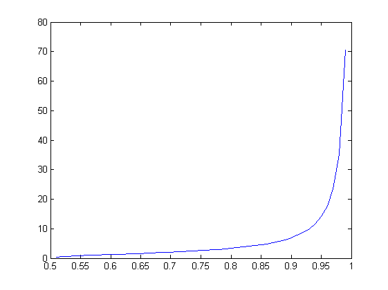
Figure 1. $\alpha\mapsto C_{1}(\alpha)$

2. Using the constant $C_{1},C_{2}$ we give the main results and at the end of this paper we give the numerical of these constants (see Figure 1,2,3, 4.)

Proof.

It is easy to calculate that

$$\int^{t}_{0}\int^{s}_{0}\int^{t}_{0}\int^{s}_{0} Q^{\alpha}(t,y_{1},y_{2})Q^{\beta}(s,u_{1},u_{2})(y_{1}y_{2})^{-\frac{1}{2}\alpha}(u_{1}u_{2})^{-\frac{1}{2}\beta}du_{2}dy_{2}du_{1}dy_{1}$$

$$=\int^{t}_{0}\int^{t}_{0}Q^{\alpha}(t,y_{1},y_{2})(y_{1},y_{2})^{-\frac{1}{2}\alpha}dy_{1}dy_{2}\int^{s}_{0}\int^{s}_{0}Q^{\beta}(s,u_{1},u_{2})(u_{1},u_{2})^{-\frac{1}{2}\beta}du_{1}du_{2}$$

$$=d_{\alpha}c^{2}_{\alpha^{\prime}}\int^{t}_{0}\int^{t}_{0}\int^{t}_{y_{1}\vee y_{2}}(y_{1}y_{2})^{-\alpha}u^{\alpha}(u-y_{1})^{\frac{1}{2}\alpha-1}(u-y_{2})^{\frac{1}{2}\alpha-1}dudy_{1}dy_{2}$$

$$\quad\times d_{\beta}c^{2}_{\beta^{\prime}}\int^{s}_{0}\int^{s}_{0}\int^{s}_{u_{1}\vee u_{2}}(u_{1}u_{2})^{-\beta}u^{\beta}(u-u_{1})^{\frac{1}{2}\beta-1}(u-u_{2})^{\frac{1}{2}\beta-1}dudy_{1}dy_{2}$$

$$=d_{\alpha}c^{2}_{\alpha^{\prime}}d_{\beta}c^{2}_{\beta^{\prime}}B^{2}(1-\alpha,\frac{1}{2}\alpha)B^{2}(1-\beta,\frac{1}{2}\beta)ts=C_{1}(\alpha)C_{1}(\beta)ts,$$

and

$$\int^{t}_{0}\int^{s}_{0}\int^{t}_{0}\int^{s}_{0} Q^{\alpha}(t,y_{1},y_{2})Q^{\beta}(s,u_{1},u_{2})(y_{1}\vee y_{2})^{\frac{1}{2}\alpha}(y_{1}\wedge y_{2})^{-\frac{1}{2}\alpha}|y_{1}-y_{2}|^{\alpha-1}$$

$$\qquad\cdot(u_{1}\vee u_{2})^{\frac{1}{2}\beta}(u_{1}\wedge u_{2})^{-\frac{1}{2}\beta}|u_{1}-u_{2}|^{\beta-1}du_{2}dy_{2}du_{1}dy_{1}$$

$$=d_{\alpha}c^{2}_{\alpha^{\prime}}[\int^{t}_{0}\int^{u}_{0}\int^{u}_{0}(y_{1}y_{2})^{-\frac{1}{2}\alpha}u^{\alpha}(u-y_{1})^{\frac{1}{2}\alpha-1}(u-y_{2})^{\frac{1}{2}\alpha-1}$$

$$\qquad\cdot(y_{1}\vee y_{2})^{\frac{1}{2}\alpha}(y_{1}\wedge y_{2})^{-\frac{1}{2}\alpha}|y_{1}-y_{2}|^{\alpha-1}dy_{1}dy_{2}du]$$

$$\quad\times d_{\beta}c^{2}_{\beta^{\prime}}[\int^{s}_{0}\int^{u}_{0}\int^{u}_{0}(u_{1}u_{2})^{-\frac{1}{2}\beta}u^{\beta}(u-u_{1})^{\frac{1}{2}\beta-1}(u-u_{2})^{\frac{1}{2}\beta-1}$$

$$\qquad\cdot(u_{1}\vee u_{2})^{\frac{1}{2}\beta}(u_{1}\wedge u_{2})^{-\frac{1}{2}\beta}|u_{1}-u_{2}|^{\beta-1}du_{1}du_{2}du]$$

$$=\frac{C_{2}(\alpha)}{\alpha}t^{2\alpha}\frac{C_{2}(\beta)}{\beta}t^{2\beta}.$$

Then for all $t\in[0,T],s\in[0,S]$, we have,

$$\int^{t}_{0}\int^{s}_{0}\int^{t}_{0}\int^{s}_{0} Q^{\alpha}(t,y_{1},y_{2})Q^{\beta}(s,u_{1},u_{2})\zeta(y_{1},y_{2},u_{1},u_{2})du_{2}dy_{2}du_{1}dy_{1}$$

$$=k_{1}C_{1}(\alpha)C_{1}(\beta)ts+k_{2}\frac{C_{2}(\alpha)C_{2}(\beta)}{\alpha\beta}t^{2\alpha}s^{2\beta}.$$

On the other hand,

$$\int^{t}_{0}\int^{s}_{0} \int^{t}_{0}\int^{s}_{0}\zeta^{2}(y_{1},y_{2},u_{1},u_{2})du_{2}dy_{2}du_{1}dy_{1}$$

$$=\int^{t}_{0}\int^{s}_{0}\int^{t}_{0}\int^{s}_{0}k_{1}^{2}(y_{1}y_{2})^{-\alpha}(u_{1}u_{2})^{-\beta}du_{2}dy_{2}du_{1}dy_{2}$$

$$\quad+\int^{t}_{0}\int^{s}_{0}\int^{t}_{0}\int^{s}_{0}k_{2}^{2}(y_{1}\vee y_{2})^{\alpha}(y_{1}\wedge y_{2})^{-\alpha}|y_{1}-y_{2}|^{2\alpha-2}$$

$$\qquad\qquad\qquad\cdot(u_{1}\vee u_{2})^{\beta}(y_{1}\wedge u_{2})^{-\beta}|u_{1}-u_{2}|^{2\beta-2}du_{2}dy_{2}du_{1}dy_{2}$$

$$\quad+\int^{t}_{0}\int^{s}_{0}\int^{t}_{0}\int^{s}_{0}2k_{1}k_{2}(y_{1}y_{2})^{-\frac{1}{2}\alpha}(y_{1}\vee y_{2})^{\frac{1}{2}\alpha}(y_{1}\wedge y_{2})^{-\frac{1}{2}\alpha}|y_{1}-y_{2}|^{\alpha-1}$$

$$\qquad\qquad\qquad\cdot(u_{1}u_{2})^{-\frac{1}{2}\beta}(u_{1}\vee u_{2})^{\frac{1}{2}\beta}(u_{1}\wedge u_{2})^{-\frac{1}{2}\beta}|u_{1}-u_{2}|^{\beta-1}du_{2}dy_{2}du_{1}dy_{2}$$

$$:=I_{1}+I_{2}+I_{3},$$

where

$$I_{1} =k_{1}^{2}\int^{t}_{0}\int^{t}_{0}(y_{1}y_{2})^{-\alpha}dy_{1}dy_{2}\int^{s}_{0}\int^{s}_{0}(u_{1}u_{2})^{-\beta}du_{1}du_{2}$$

$$=\frac{t^{2-2\alpha}s^{2-2\beta}}{(1-\alpha)^{2}(1-\beta)^{2}}k_{1}^{2}.$$

$$I_{2} =k_{2}^{2}(\int^{t}_{0}\int^{t}_{0}(y_{1}\vee y_{2})^{\alpha}(y_{1}\wedge y_{2})^{-\alpha}|y_{1}-y_{2}|^{2\alpha-2}dy_{1}dy_{2})$$

$$\qquad\qquad\cdot(\int^{s}_{0}\int^{s}_{0}(u_{1}\vee u_{2})^{\beta}(y_{1}\wedge u_{2})^{-\beta}|u_{1}-u_{2}|^{2\beta-2}du_{1}du_{1})$$

$$=k_{2}^{2}\left[\int^{t}_{0}\int^{y_{2}}_{0}y_{2}^{\alpha}y_{1}^{-\alpha}(y_{2}-y_{1})^{2\alpha-2}dy_{1}dy_{2}+\int^{t}_{0}\int^{t}_{y_{2}}y_{1}^{\alpha}y_{2}^{-\alpha}(y_{1}-y_{2})^{2\alpha-2}dy_{1}dy_{2}\right]$$

$$\qquad\cdot\left[\int^{s}_{0}\int^{u_{2}}_{0}u_{2}^{\beta}u_{1}^{-\beta}(u_{2}-u_{1})^{2\beta-2}du_{1}du_{2}+\int^{u}_{0}\int^{s}_{u_{2}}u_{1}^{\beta}u_{2}^{-\beta}(u_{1}-u_{2})^{2\beta-2}du_{1}du_{2}\right]$$

$$=k_{2}^{2}(2\int^{t}_{0}y_{2}^{2\alpha-1}dy_{2}\int^{1}_{0}u^{-\alpha}(1-u)^{2\alpha-2}du)\cdot(2\int^{s}_{0}u_{2}^{2\beta-1}du_{2}\int^{1}_{0}u^{-\beta}(1-u)^{2\beta-2}du)$$

$$=\frac{k_{2}^{2}}{\alpha\beta}B(1-\alpha,2\alpha-1)B(1-\beta,2\beta-1)t^{2\alpha}s^{2\beta}.$$

$$I_{3} =2k_{1}k_{2}(\int^{t}_{0}\int^{t}_{0}(y_{1}y_{2})^{-\frac{1}{2}\alpha}(y_{1}\vee y_{2})^{\frac{1}{2}\alpha}(y_{1}\wedge y_{2})^{-\frac{1}{2}\alpha}|y_{1}-y_{2}|^{\alpha-1}dy_{1}dy_{2})$$

$$\qquad\cdot(\int^{s}_{0}\int^{s}_{0}(u_{1}u_{2})^{-\frac{1}{2}\beta}(u_{1}\vee u_{2})^{\frac{1}{2}\beta}(u_{1}\wedge u_{2})^{-\frac{1}{2}\beta}|u_{1}-u_{2}|^{\beta-1}du_{1}du_{2})$$

$$=2k_{1}k_{2}(\int^{t}_{0}\int^{y_{2}}_{0}y_{1}^{-\alpha}(y_{2}-y_{1})^{\alpha-1}dy_{1}dy_{2}+\int^{t}_{0}\int_{y_{2}}^{t}y_{2}^{-\alpha}(y_{1}-y_{2})^{\alpha-1}dy_{1}dy_{2})$$

$$\qquad\cdot(\int^{s}_{0}\int^{u_{2}}_{0}u_{1}^{-\beta}(u_{2}-u_{1})^{\beta-1}du_{1}du_{2}+\int^{s}_{0}\int_{u_{2}}^{s}u_{2}^{-\beta}(u_{1}-u_{2})^{\beta-1}du_{1}du_{2})$$

$$=2k_{1}k_{2}(2\int^{t}_{0}dy_{1}\int^{1}_{0}u^{-\alpha}|1-u|^{\alpha-1}du)\cdot(2\int^{s}_{0}du_{1}\int^{1}_{0}u^{-\beta}|1-u|^{\beta-1}du)$$

$$=8k_{1}k_{2}B(1-\alpha,\alpha)B(1-\beta,\beta)ts.$$

Hence,

$$\int^{t}_{0}\int^{s}_{0}\int^{t}_{0}\int^{s}_{0}\zeta^{2}(y_{1},y_{2},u_{1},u_{2})du_{2}dy_{2}du_{1}dy_{1}=\frac{k_{1}^{2}}{(1-\alpha)^{2}(1-\beta)^{2}}t^{2-2\alpha}s^{2-2\beta}$$

$$\quad+\frac{k_{2}^{2}}{\alpha\beta}B(1-\alpha,2\alpha-1)B(1-\beta,2\beta-1)t^{2\alpha}s^{2\beta}+8k_{1}k_{2}B(1-\alpha,\alpha)B(1-\beta,\beta)ts,$$

for all $\zeta\in\mathcal{K}$. It follows that

$$f(t,s,k_{1},k_{2}) =2E(Z^{\alpha,\beta}(t,s)-M_{t,s}(\zeta))^{2}$$

$$=t^{2\alpha}s^{2\beta}+4\int^{t}_{0}\int^{s}_{0}\int^{t}_{0}\int^{s}_{0}\zeta^{2}(y_{1},y_{2},u_{1},u_{2})du_{2}dy_{2}du_{1}dy_{1}$$

$$-8\int^{t}_{0}\int^{s}_{0}\int^{t}_{0}\int^{s}_{0}Q^{\alpha}(t,y_{1},y_{2})Q^{\beta}(s,u_{1},u_{2})\zeta(y_{1},y_{2},u_{1},u_{2})du_{2}dy_{2}du_{1}dy_{1}$$

$$=a(k_{2})t^{2\alpha}s^{2\beta}-8k_{1}b(k_{2})ts+4k_{1}^{2}\frac{t^{2-2\alpha}s^{2-2\beta}}{(1-\alpha)^{2}(1-\beta)^{2}}.$$

This completes the proof.
∎

3. The maximum value of $f(t,s,k_{1},k_{2})$

In this section, in order to obtain the optimal approximation with $k_{1},k_{2}>0$. We need to find the maximum value point $P_{0}(t_{0},s_{0})$ in the open rectangle interval $(0,T)\times(0,S)$, and the maximum value point at the boundary of rectangle interval $[0,T]\times[0,S]$. Thus, we can get the $\sup\limits_{t\in[0,T],s\in[0,S]}f(t,s,k_{1},k_{2}).$

Lemma 3.1.

The function $f(t,s,k_{1}.k_{2})$ at the open rectangle interval $(0,T)\times(0,S)$ can’t get the maximum value point $P_{0}(t_{0},s_{0})$, $t_{0}\in(0,T),s_{0}\in(0,S)$.

Proof.

If the function $f(t,s,k_{1},k_{2})$ have maximum value point $P_{0}(t_{0},s_{0})$, $t_{0}\in(0,T),s_{0}\in(0,S)$, then $P_{0}(t_{0},s_{0})$ must be the stagnation point of the function

$$(t,s)\mapsto f(t,s,k_{1},k_{2}).$$

That is,

$$\frac{\partial f(t,s,k_{1},k_{2})}{\partial t}|_{P_{0}(t_{0},s_{0})}=0,~{}~{}~{}\frac{\partial f(t,s,k_{1},k_{2})}{\partial s}|_{P_{0}(t_{0},s_{0})}=0,$$

Solving equations set:

$$\frac{\partial f(t,s,k_{1},k_{2})}{\partial t} =2t^{1-2\alpha}s^{2-2\beta}(\alpha a(k_{2})t^{4\alpha-2}s^{4\beta-2}$$

$$\quad-4k_{1}b(k_{2})t^{2\alpha-1}s^{2\beta-1}+\frac{4k_{1}^{2}}{(1-\alpha)(1-\beta)^{2}})=0,$$

$$\frac{\partial f(t,s,k_{1},k_{2})}{\partial s} =2t^{2-2\alpha}s^{1-2\beta}(\beta a(k_{2})t^{4\alpha-2}s^{4\beta-2}$$

$$\quad-4k_{1}b(k_{2})t^{2\alpha-1}s^{2\beta-1}+\frac{4k_{1}^{2}}{(1-\alpha)^{2}(1-\beta)})=0.$$

Let $x=t^{2\alpha-1}s^{2\beta-1},$ elementary calculation can obtain

$$x=\frac{k_{1}}{b(k_{2})(1-\alpha)^{2}(1-\beta)^{2}},$$

and

$$\sqrt{a(k_{2})}=2b(k_{2})(1-\alpha)(1-\beta).$$

Hence, we have

$$f(t_{0},s_{0},k_{1},k_{2})=t_{0}s_{0}[a(k_{2})\frac{k_{1}}{b(k_{2})(1-\alpha)^{2}(1-\beta)^{2}}-4k_{1}b(k_{2})]=0.$$

But $f(\varepsilon,\varepsilon,0,0)=\varepsilon^{2}>0$, for any $\varepsilon>0$. That is contradiction. Therefore, the function $f(t,s,k_{1},k_{2})$ at the open rectangle interval$(0,T)\times(0,S)$ can’t get the maximum value point $P_{0}(t_{0},s_{0})$, $t_{0}\in(0,T),s_{0}\in(0,S)$. ∎

At the boundary $0\times[0,S]$, and $[0,T]\times 0$, we have $f(t,s,k_{1},k_{2})=0$. So, we need to consider the case of extremum value point on the boundary $T\times[0,S]$ and $[0,T]\times S$, with $k_{1},k_{2}>0$. We only think about the case of the boundary $T\times[0,S]$. In the same way, we can get case of the boundary $[0,T]\times S$.

It follows from Theorem 2.1, we know that

(3.1) $$f(T,s,k_{1},k_{2})=a(k_{2})T^{2\alpha}s^{2\beta}-8k_{1}b(k_{2})Ts+4k_{1}^{2}\frac{T^{2-2\alpha}s^{2-2\beta}}{(1-\alpha)^{2}(1-\beta)^{2}},$$

for all $s\in[0,S]$. Differentiating (3.1) with respect to $s$ leads to

(3.2) $$f_{s}(T,s,k_{1},k_{2})=2\beta a(k_{2})T^{2\alpha}s^{2\beta-1}-8k_{1}b(k_{2})T+\frac{8k_{1}^{2}}{(1-\alpha)^{2}(1-\beta)}T^{2-2\alpha}s^{1-2\beta}.$$

Let $f_{s}(T,s,k_{1},k_{2})=0$ and $x=k_{1}s^{1-2\beta}$, which implies that

(3.3) $$F(x):=\beta a(k_{2})T^{2\alpha}-4b(k_{2})Tx+\frac{4T^{2-2\alpha}x^{2}}{(1-\alpha)^{2}(1-\beta)}=0$$

and the discriminant $\Delta$ of the quadratic function $F(x)$ is

$$\Delta=16T^{2}((b(k_{2}))^{2}-\frac{\beta a(k_{2})}{(1-\alpha)^{2}(1-\beta)}).$$

If $\Delta\leq 0$, then

(3.4) $$\begin{split}\sup_{s\in[0,S]}f(T,s,k_{1},k_{2})&=f(T,S,k_{1},k_{2})\\ &=T^{2\alpha}S^{2\beta}a(k_{2})-8k_{1}b(k_{2})TS+4k_{1}^{2}\frac{T^{2-2\alpha}S^{2-2\beta}}{(1-\alpha)^{2}(1-\beta)^{2}}.\end{split}$$

Using the same method, on the boundary $[0,T]\times S$, we have

$$\sup_{t\in[0,T]}f(t,S,k_{1},k_{2})=f(T,S,k_{1},k_{2}).$$

If $\Delta>0$, then the equation (3.3) has two real roots as follows

$$x_{1}=\frac{(1-\alpha)^{2}(1-\beta)}{2T^{1-2\alpha}}(b(k_{2})+\sqrt{b^{2}(k_{2})-\frac{\beta a(k_{2})}{(1-\alpha)^{2}(1-\beta)}}),$$

and

$$x_{2}=\frac{(1-\alpha)^{2}(1-\beta)}{2T^{1-2\alpha}}(b(k_{2})-\sqrt{b^{2}(k_{2})-\frac{\beta a(k_{2})}{(1-\alpha)^{2}(1-\beta)}}),$$

which says $s_{1}=k_{1}^{\frac{1}{2\alpha-1}}x_{1}^{-\frac{1}{2\alpha-1}}$, and $s_{2}=k_{1}^{\frac{1}{2\alpha-1}}x_{2}^{-\frac{1}{2\alpha-1}}$ are two stagnation points of the function $s\mapsto f(T,s,k_{1},k_{2})$. Hence, $s_{1},s_{2}$ are the points of local maximum and minimum, respectively, since the monotonicity of the function $s\mapsto f(T,s,k_{1},k_{2})$. This implies that

(3.5) $$\begin{split}&\sup_{s\in[0,S]}f(T,s,k_{1},k_{2})=f(T,S,k_{1},k_{2}),\qquad\textmd{if}\quad s_{1}\geq S,\\ &\sup_{s\in[0,S]}f(T,s,k_{1},k_{2})=\max\{f(T,s_{1},k_{1},k_{2}),f(T,S,k_{1},k_{2})\},\qquad\textmd{if}\quad s_{1}<S.\end{split}$$

Using the same method, on the boundary $[0,T]\times S$, we can find a $t_{1}$, such that

(3.6) $$\begin{split}&\sup_{t\in[0,T]}f(t,S,k_{1},k_{2})=f(T,S,k_{1},k_{2}),\qquad\textmd{if}\quad t_{1}\geq T,\\ &\sup_{t\in[0,T]}f(t,S,k_{1},k_{2})=\max\{f(t_{1},S,k_{1},k_{2}),f(T,S,k_{1},k_{2})\},\qquad\textmd{if}\quad t_{1}<T.\end{split}$$

4. The optimal approximation, case $\Delta\leq 0$

Theorem 4.1.

If $\Delta\leq 0$, then we have

$$\inf_{\zeta\in\mathcal{K}}\sup_{T\times[0,S]}f(t,s,k_{1},k_{2})=T^{2\alpha}S^{2\beta}a(k^{*}_{2})-8k^{*}_{1}b(k^{*}_{2})TS+4(k^{*}_{1})^{2}\frac{T^{2-2\alpha}S^{2-2\beta}}{(1-\alpha)^{2}(1-\beta)^{2}},$$

where

$$\mathcal{K}=\{\zeta(y_{1},y_{2},u_{1},u_{2})= k^{*}_{1}(y_{1},y_{2})^{-\frac{1}{2}\alpha}(u_{1},u_{2})^{-\frac{1}{2}\beta}+k^{*}_{2}(y_{1}\vee y_{2})^{\frac{1}{2}\alpha}(y_{1}\wedge y_{2})^{-\frac{1}{2}\alpha}|y_{1}-y_{2}|^{\alpha-1}$$

$$\quad\cdot(u_{1}\vee u_{2})^{\frac{1}{2}\beta}(u_{1}\wedge u_{2})^{-\frac{1}{2}\beta}|u_{1}-u_{2}|^{\beta-1},k_{1},k_{2}>0\}$$

and $(k_{1}^{*},k_{2}^{*})$ is the stagnation point of the function

$$(k_{1},k_{2})\mapsto f(T,S,k_{1},k_{2}),$$

here

(4.1) $$\begin{split}k_{1}^{*}=&\frac{4B(1-\alpha,\alpha)B(1-\beta,\beta)C_{2}(\alpha)C_{2}(\beta)-B(1-\alpha,2\alpha-1)B(1-\beta,2\beta-1)C_{1}(\alpha)C_{1}(\beta)}{8\alpha\beta(1-\alpha)^{2}(1-\beta)^{2}B^{2}(1-\alpha,\alpha)B^{2}(1-\beta,\beta)-B(1-\alpha,2\alpha-1)B(1-\beta,2\beta-1)}\\ &\quad\times(1-\alpha)^{2}(1-\beta)^{2}T^{2\alpha-1}S^{2\beta-1},\end{split}$$

(4.2) $$k_{2}^{*}=\frac{C_{2}(\alpha)C_{2}(\beta)-4\alpha\beta(1-\alpha)^{2}(1-\beta)^{2}B(1-\alpha,\alpha)B(1-\beta,\beta)C_{1}(\alpha)C_{1}(\beta)}{B(1-\alpha,2\alpha-1)B(1-\beta,2\beta-1)-8\alpha\beta(1-\alpha)^{2}(1-\beta)^{2}B^{2}(1-\alpha,\alpha)B^{2}(1-\beta,\beta)}.$$

Proof.

It follows from equation (3.4), when $\Delta\leq 0$,

$$\sup_{s\in[0,S]}f(T,s,k_{1},k_{2})=T^{2\alpha}S^{2\beta}a(k_{2})-8k_{1}b(k_{2})TS+4(k_{1})^{2}\frac{T^{2-2\alpha}S^{2-2\beta}}{(1-\alpha)^{2}(1-\beta)^{2}}\\$$

for all $k_{1},k_{2}\geq 0$. Let now $(k_{1}^{*},k_{2}^{*})$ be the stagnation point of the function

$$(k_{1},k_{2})\mapsto f(T,S,k_{1},k_{2}).$$

An elementary calculation can obtain $k_{1}^{*},k_{2}^{*}$ which can be denoted by (4.1) and (4.2), and the Hessian matrix $\mathbf{H}$ as follows

$$\mathbf{H}=\left(\begin{array}[]{ccc}\frac{\partial^{2}f(T,S,k_{1}k_{2})}{\partial k_{1}^{2}}&\frac{\partial^{2}f(T,S,k_{1}k_{2})}{\partial k_{1}\partial k_{2}}\\ \frac{\partial^{2}f(T,S,k_{1}k_{2})}{\partial k_{2}\partial k_{1}}&\frac{\partial^{2}f(T,S,k_{1}k_{2})}{\partial k_{2}^{2}}\\ \end{array}\right)$$

and

$$\frac{\partial^{2}f(T,S,k_{1}k_{2})}{\partial k_{1}^{2}}=\frac{8T^{2-2\alpha}S^{2-2\beta}}{(1-\alpha)^{2}(1-\beta)^{2}}>0,$$

$$\frac{\partial^{2}f(T,S,k_{1}k_{2})}{\partial k_{1}\partial k_{2}} =\frac{\partial^{2}f(T,S,k_{1}k_{2})}{\partial k_{2}\partial k_{1}}$$

$$=32TSB(1-\alpha,\alpha)B(1-\beta,\beta),$$

$$\frac{\partial^{2}f(T,S,k_{1}k_{2})}{\partial k_{2}^{2}}=\frac{8T^{2\alpha}S^{2\beta}}{\alpha\beta}B(1-\alpha,2\alpha-1)B(1-\beta,2\beta-1).$$

So,

$$|\mathbf{H}|=64T^{2}S^{2}(\frac{B(1-\alpha,2\alpha-1)B(1-\beta,2\beta-1)}{\alpha(1-\alpha)^{2}\beta(1-\beta)^{2}}-16B^{2}(1-\alpha,\alpha)B^{2}(1-\beta,\beta))>0$$

for all $\frac{1}{2}<\alpha,\beta<1$, since $B^{2}(1-\alpha,\alpha)<\frac{B(1-\alpha,2\alpha-1)}{1-\alpha}$. This means that the minimal value of $(k_{1},k_{2})\mapsto f(T,S,k_{1},k_{2})$ is achieved at point $(k_{1}^{*},k_{2}^{*})$. This completes the proof. ∎

5. The optimal approximation, case $\Delta>0$

Lemma 5.1.

If $\Delta>0$, then we have

$$s_{1}(k_{1}^{*},k_{2}^{*})<S,$$

and

$$s_{2}(k_{1}^{*},k_{2}^{*})<S,$$

where $(k_{1}^{*},k_{2}^{*})$ is the stagnation point of the function $(k_{1},k_{2})\mapsto\sup_{s\in[0,S]}f(T,s,k_{1},k_{2})$.

Proof.

We split the proof in two steps.
Step one. It is easy to obtain that,

(5.1) $$\frac{2}{s_{1}^{2\beta-1}}>\frac{1}{s_{1}^{2\beta-1}}+\frac{1}{s_{2}^{2\beta-1}}=\frac{x_{1}+x_{2}}{k_{1}}=\frac{b(k_{2})(1-\alpha)^{2}(1-\beta)}{T^{1-2\alpha}k_{1}}.$$

since $s_{2}>s_{1}$. Hence, when $k_{1}=k_{1}^{*}$ and $k_{2}=k_{2}^{*}$,

(5.2) $$\begin{split}\frac{b(k_{2}^{*})(1-\alpha)^{2}(1-\beta)}{T^{1-2\alpha}k^{*}_{1}}&=\frac{(C_{1}(\alpha)C_{1}(\beta)-4k^{*}_{2}B(1-\alpha,\alpha)B(1-\beta,\beta))(1-\alpha)^{2}(1-\beta)}{T^{1-2\alpha}k^{*}_{1}}\\ &=\frac{S^{1-2\beta}}{1-\beta}>\frac{2}{S^{2\beta-1}}\end{split}$$

for $\beta\in(\frac{1}{2},1)$. This proves that $s_{1}(k_{1}^{*},k_{2}^{*})<S$.
Step two.

$$\frac{\partial f(T,s,k_{1}^{*},k_{2}^{*})}{\partial s}=2\beta a(k_{2}^{*})T^{2\alpha}s^{2\beta-1}-8k^{*}_{1}b(k^{*}_{2})T+\frac{8(k^{*}_{1})^{2}}{(1-\alpha)^{2}(1-\beta)}T^{2-2\alpha}s^{1-2\beta}$$

$$=2\beta a(k_{2}^{*})T^{2\alpha}s^{2\beta-1}-8\frac{b(k_{2}^{*})(1-\alpha)^{2}(1-\beta)^{2}}{T^{1-2\alpha}s^{1-2\beta}}b(k^{*}_{2})T+\frac{8(\frac{b(k_{2}^{*})(1-\alpha)^{2}(1-\beta)^{2}}{T^{1-2\alpha}s^{1-2\beta}})^{2}}{(1-\alpha)^{2}(1-\beta)}T^{2-2\alpha}s^{1-2\beta}$$

$$=2\beta T^{2\alpha}s^{2\beta-1}(a(k_{2}^{*})-4b^{2}(k_{2}^{*})(1-\alpha)^{2}(1-\beta)^{2}),$$

since,

$$k^{*}_{1}=\frac{b(k_{2}^{*})(1-\alpha)^{2}(1-\beta)^{2}}{T^{1-2\alpha}S^{1-2\beta}},~{}~{}~{}\textmd{and}~{}~{}~{}4b^{2}(k_{2}^{*})\leq\frac{a(k_{2}^{*})}{(1-\alpha)^{2}(1-\beta)^{2}}.$$

Hence,

$$\frac{\partial f(T,s,k_{1}^{*},k_{2}^{*})}{\partial s}|_{s=S}>0.$$

Thus, $S<s_{1}$ or $S>s_{2}$. By step one, we know $S>s_{1}$, so $s_{2}(k_{1}^{*},k_{2}^{*})<S$. ∎

Lemma 5.2.

Denote

$$h(k_{1},k_{2})=f(T,s_{1},k_{1},k_{2})-f(T,S,k_{1},k_{2}).$$

Then the equation $h(k_{1},k_{2})=0$ has two solutions $k_{1}^{{}^{\prime}}$ and $\overline{k_{1}}$, which satisfy $0<k_{1}^{{}^{\prime}}<\overline{k_{1}}$, $\frac{\partial h}{\partial k_{1}}|_{k_{1}=k_{1}^{{}^{\prime}}}>0$ and $\frac{\partial h}{\partial k_{1}}|_{k_{1}=\overline{k_{1}}}=0.$

Proof.

By Theorem 2.1 , we have

$$f(T,s_{1},k_{1},k_{2}) =T^{2\alpha}s_{1}^{2\beta}a(k_{2})-8k_{1}b(k_{2})Ts_{1}+4k_{1}^{2}\frac{T^{2-2\alpha}s_{1}^{2-2\beta}}{(1-\alpha)^{2}(1-\beta)^{2}}$$

$$=T^{2\alpha}(\frac{k_{1}}{x_{1}})^{\frac{2\beta}{2\beta-1}}a(k_{2})-8k_{1}b(k_{2})T(\frac{k_{1}}{x_{1}})^{\frac{1}{2\beta-1}}+4k_{1}^{2}\frac{T^{2-2\alpha}(\frac{k_{1}}{x_{1}})^{\frac{2-2\beta}{2\beta-1}}}{(1-\alpha)^{2}(1-\beta)^{2}}$$

$$:=k_{1}^{\frac{\beta}{\beta-\frac{1}{2}}}\varphi(k_{2})=k_{1}^{\frac{2\beta}{2\beta-1}}\varphi(k_{2}).$$

Let $h(k_{1},k_{2})=0$, which implies that

(5.3) $$k_{1}^{\frac{2\beta}{2\beta-1}}\varphi(k_{2})=T^{2\alpha}S^{2\beta}a(k_{2})-8k_{1}b(k_{2})TS+4k_{1}^{2}\frac{T^{2-2\alpha}S^{2-2\beta}}{(1-\alpha)^{2}(1-\beta)^{2}}=f(T,S,k_{1},k_{2}).\\$$

Differentiating (5.3) with respect to $k_{1}$

(5.4) $$\frac{2\beta}{2\beta-1}k_{1}^{\frac{1}{2\beta-1}}\varphi(k_{2})=-8b(k_{2})TS+8k_{1}\frac{T^{2-2\alpha}S^{2-2\beta}}{(1-\alpha)^{2}(1-\beta)^{2}}.\\$$

multiplying by $\frac{2\beta}{(2\beta-1)k_{1}}$ on both side of (5.3) leads to

(5.5) $$\frac{2\beta}{2\beta-1}k_{1}^{\frac{1}{2\beta-1}}\varphi(k_{2})=\frac{2\beta a(k_{2})T^{2\alpha}S^{2\beta}}{(2\beta-1)k_{1}}-\frac{16\beta b(k_{2})TS}{2\beta-1}+8\beta k_{1}\frac{T^{2-2\alpha}S^{2-2\beta}}{(2\beta-1)(1-\alpha)^{2}(1-\beta)^{2}}.\\$$

It follows that

$$-8b(k_{2})TS +8k_{1}\frac{T^{2-2\alpha}S^{2-2\beta}}{(1-\alpha)^{2}(1-\beta)^{2}}$$

$$=\frac{2\beta a(k_{2})T^{2\alpha}S^{2\beta}}{(2\beta-1)k_{1}}-\frac{16\beta b(k_{2})TS}{2\beta-1}+8\beta k_{1}\frac{T^{2-2\alpha}S^{2-2\beta}}{(2\beta-1)(1-\alpha)^{2}(1-\beta)^{2}}.$$

This implies that

(5.6) $$(4\beta-4)T^{2-2\alpha}S^{2-2\beta}k_{1}^{2}+4b(k_{2})TS(1-\alpha)^{2}(1-\beta)^{2}k_{1}-\beta a(k_{2})(1-\alpha)^{2}(1-\beta)^{2}T^{2\alpha}S^{2\beta}=0.$$

This is a quadratic equation in $k_{1}$ with the two roots

$$\overline{k_{1}}=\frac{b(k_{2})(1-\alpha)^{2}(1-\beta)^{2}+\sqrt{D}}{2(1-\beta)T^{1-2\alpha}S^{1-2\beta}},$$

$$\underline{k_{1}}=\frac{b(k_{2})(1-\alpha)^{2}(1-\beta)^{2}-\sqrt{D}}{2(1-\beta)T^{1-2\alpha}S^{1-2\beta}},$$

since

$$D=b^{2}(k_{2})(1-\alpha)^{4}(1-\beta)^{4}-\beta a(k_{2})(1-\beta)^{3}(1-\alpha)^{2}>0.$$

It is easy to check that $\overline{k_{1}}$ is the solution to the equation set

$$\left\{\begin{array}[]{ll}h(k_{1},k_{2})=0,\\ \frac{\partial h}{\partial k_{1}}(k_{1},k_{2})=0.\end{array}\right.$$

In the follows, we will prove that $\underline{k_{1}}$ is not the solution of the equation $h(k_{1},k_{2})=0$. In fact,

$$h(\underline{k_{1}},k_{2})=f(T,s_{1},\underline{k_{1}},k_{2})-f(T,S,\underline{k_{1}},k_{2})$$

$$=x_{2}^{\frac{2\beta}{2\beta-1}}\varphi(k_{2})S^{2\beta}-a(k_{2})T^{2\alpha}S^{2\beta}+8b(k_{2})TS^{2\beta}x_{2}-\frac{4T^{2-2\alpha}}{(1-\alpha)^{2}(1-\beta)^{2}}x_{2}^{2}S^{2\beta}$$

$$=S^{2\beta}(x_{2}^{\frac{2\beta}{2\beta-1}}\varphi(k_{2})-a(k_{2})T^{2\alpha}+8b(k_{2})Tx_{2}-\frac{4T^{2-2\alpha}}{(1-\alpha)^{2}(1-\beta)^{2}}x_{2}^{2})$$

$$=\frac{2\beta-1}{1-\beta}S^{2\beta}((\frac{x_{2}}{x_{1}})^{\frac{2\beta}{2\beta-1}}(4b(k_{2})Tx_{1}-a(k_{2})T^{2\alpha})-(4b(k_{2})Tx_{2}-a(k_{2})T^{2\alpha})),$$

since

$$\varphi(k_{2})=a(k_{2})T^{2\alpha}x_{1}^{-\frac{2\beta}{2\beta-1}}-8b(k_{2})x_{1}^{\frac{1}{2\beta-1}}+\frac{4T^{2-2\alpha}}{(1-\alpha)^{2}(1-\beta)^{2}}x_{1}^{2\beta-2}.$$

By (3.3), we have

$$x_{1}+x_{2}=b(k_{2})T^{2\alpha-1}(1-\alpha)^{2}(1-\beta),\qquad x_{1}x_{2}=\frac{1}{4}\beta a(k_{2})T^{4\alpha-2}(1-\alpha)^{2}(1-\beta),$$

since $x_{1},x_{2}$ are the root of equation $\beta a(k_{2})T^{2\alpha}-4b(k_{2})Tx+\frac{4T^{2-2\alpha}x^{2}}{(1-\alpha)^{2}(1-\beta)}=0.$ Thus,

$$\frac{4b(k_{2})Tx_{1}}{a(k_{2})T^{2\alpha}}=\beta\frac{x_{1}+x_{2}}{x_{2}},\qquad\frac{4b(k_{2})Tx_{2}}{a(k_{2})T^{2\alpha}}=\beta\frac{x_{1}+x_{2}}{x_{1}}.$$

Let $x=\frac{x_{2}}{x_{1}}\in(0,1)$. Then

$$( \frac{x_{2}}{x_{1}})^{\frac{2\beta}{2\beta-1}}(4b(k_{2})Tx_{1}-a(k_{2})T^{2\alpha})-(4b(k_{2})Tx_{2}-a(k_{2})T^{2\alpha})$$

$$=a(k_{2})T^{2\alpha}((\frac{x_{2}}{x_{1}})^{\frac{2\beta}{2\beta-1}}(\frac{\beta(x_{1}+x_{2})}{x_{2}}-1)-(\frac{\beta(x_{1}+x_{2})}{x_{1}}-1))$$

$$=a(k_{2})T^{2\alpha}(x^{\frac{2\beta}{2\beta-1}}(\beta x^{-1}+\beta-1)-\beta-\beta x+1)$$

$$:=a(k_{2})T^{2\alpha}\phi(x).$$

It is easy to check $\phi(x)>0$. In fact, $\phi(0)=1-\beta$, $\phi(1)=0$, and $\phi^{{}^{\prime}}(0)=-\beta$, $\phi^{{}^{\prime}}(1)=0$

$$\phi^{{}^{\prime\prime}}(x)=\frac{2\beta(1-\beta)}{(2\beta-1)^{2}}x^{\frac{2-2\beta}{2\beta-1}}(x^{\frac{1-2\beta}{2\beta-1}}-1)>0$$

for all $x\in(0,1)$ since $2\beta>1$. This shows that the function $\phi(x)$ is convex on $(0,1)$ and $\phi^{{}^{\prime}}(x)$ is increasing strictly on $(0,1)$, which implies $\phi^{{}^{\prime}}(x)<0$. It follows that $\phi^{{}^{\prime}}(x)$ is decreasing strictly on $(0,1)$ and

$$\phi(x)>\phi(1)=0$$

for all $x\in(0,1)$, Thus, $h(\underline{k_{1}},k_{2})>0$.
On the other hand, $h(0,k_{2})=-a(k_{2})T^{2\alpha}S^{2\beta}<0$, it follows that the equation

$$h(k_{1},k_{2})=f(T,s_{1},k_{1},k_{2})-f(T,S,k_{1},k_{2})=0$$

admits a root, denoted by $k_{1}^{{}^{\prime}}$, on $(0,\underline{k_{1}})$. Noting that the $k_{1}\mapsto f(T,s_{1},k_{1},k_{2})$ is convex and increasing, we find that the equation

$$h(k_{1},k_{2})=f(T,s_{1},k_{1},k_{2})-f(T,S,k_{1},k_{2})=0$$

admits two roots at most since the function $k_{1}\mapsto f(T,S,k_{1},k_{2})$ is a quadratic function. Thus, $k_{1}^{{}^{\prime}}$ is unique in $(0,\underline{k_{1}})$ and $\frac{\partial h}{\partial k_{1}}|_{k_{1}=k_{1}^{{}^{\prime}}}>0$. ∎

Now, we consider $\sup_{s\in[0,S]}f(T,s,k_{1},k_{2})$ at the case $\Delta>0$.

Theorem 5.1.

If $\Delta>0$, $k_{1}^{{}^{\prime}}$ is given in Lemma 5.2. We have

$$\max\{f(T,s_{1},k_{1},k_{2}),f(T,S,k_{1},k_{2})\}=f(T,S,k_{1}^{{}^{\prime}},k_{2}).$$

Proof.

By Lemma 5.1, we have

$$\sup_{s\in[0,S]}f(T,s,k_{1},k_{2})=\max\{f(T,s_{1},k_{1},k_{2}),f(T,S,k_{1},k_{2})\}.$$

It follows from Lemma 5.2 that

$$\max\{f(T,s_{1},k_{1},k_{2}),f(T,S,k_{1},k_{2})\}=f(T,s_{1},k_{1},k_{2})1_{\{k_{1}>k_{1}^{{}^{\prime}}\}}+f(T,S,k_{1},k_{2})_{\{k_{1}<k_{1}^{{}^{\prime}}\}},$$

which implies that

$$\max\{f(T,s_{1},k_{1},k_{2}),f(T,S,k_{1},k_{2})\}=f(T,S,k_{1}^{{}^{\prime}},k_{2}),$$

since $k_{1}\mapsto f(T,s_{1},k_{1},k_{2})$ is increasing and $f(T,S,k_{1},k_{2})$ is decreasing for $k_{1}<k_{1}^{{}^{\prime}}$. ∎

Remark 3. By Theorem 5.1 and (3.5), we have

$$\sup_{s\in[0,S]}f(T,s,k_{1},k_{2})=f(T,S,k_{1}^{{}^{\prime}},k_{2}),$$

where $k_{1}^{{}^{\prime}}\in(0,\underline{k_{1}})$.
Use the same method, on the boundary $[0,T]\times S$, there also exists a $k_{1}^{{}^{\prime\prime}}>0$, such that

$$\sup_{t\in[0,T]}f(t,S,k_{1},k_{2})=f(T,S,k_{1}^{{}^{\prime\prime}},k_{2}).$$

From all above, we have

$$\sup_{t\in[0,T],s\in[0,S]}f(t,s,k_{1},k_{2})=\max\{f(T,S,k_{1}^{{}^{\prime}},k_{2}),f(T,S,k_{1}^{{}^{\prime\prime}},k_{2})\}$$

Theorem 5.2.

1)If $f(T,S,k_{1}^{{}^{\prime}},k_{2})>f(T,S,k_{1}^{{}^{\prime\prime}},k_{2})$. Then minimal value

$$\inf_{\zeta\in\mathcal{K}}\sup_{t\in[0,T],s\in[0,S]}f(t,s,k_{1},k_{2})$$

is achieved at point $(T,S,k_{1}^{{}^{\prime}},k_{2}^{{}^{\prime}})$ and equals to $f(T,S,k_{1}^{{}^{\prime}},k_{2}^{{}^{\prime}})$.
2)If $f(T,S,k_{1}^{{}^{\prime}},k_{2})<f(T,S,k_{1}^{{}^{\prime\prime}},k_{2})$. Then minimal value

$$\inf_{\zeta\in\mathcal{K}}\sup_{t\in[0,T],s\in[0,S]}f(t,s,k_{1},k_{2})$$

is achieved at point $(T,S,k_{1}^{{}^{\prime\prime}},k_{2}^{{}^{\prime\prime}})$ and equals to $f(T,S,k_{1}^{{}^{\prime\prime}},k_{2}^{{}^{\prime\prime}})$.

Proof.

1). If $f(T,S,k_{1}^{{}^{\prime}},k_{2})>f(T,S,k_{1}^{{}^{\prime\prime}},k_{2})$, then

$$\sup_{t\in[0,T],s\in[0,S]} f(t,s,k_{1},k_{2})=f(T,S,k_{1}^{{}^{\prime}},k_{2})$$

$$=T^{2\alpha}S^{2\beta}a(k_{2})-8k^{{}^{\prime}}_{1}b(k_{2})TS+4(k^{{}^{\prime}}_{1})^{2}\frac{T^{2-2\alpha}S^{2-2\beta}}{(1-\alpha)^{2}(1-\beta)^{2}}$$

$$=(\frac{4T^{2\alpha}S^{2\beta}}{\alpha\beta}B(1-\alpha,2\alpha-1)B(1-\beta,2\beta-1))k_{2}^{2}$$

$$\quad+(32k_{1}^{{}^{\prime}}TSB(1-\alpha,\alpha)B(1-\beta,\beta)-\frac{8C_{2}(\alpha)C_{2}(\beta)}{\alpha\beta}T^{2\alpha}S^{2\beta})k_{2}$$

$$\quad+T^{2\alpha}S^{2\beta}-8k_{1}^{{}^{\prime}}TSC_{1}(\alpha)C_{1}(\beta)+\frac{4(k_{1}^{{}^{\prime}})^{2}}{(1-\alpha)^{2}(1-\beta)^{2}}T^{2-2\alpha}S^{2-2\beta}.$$

This is a quadratic equation of $k_{2}$, and $\frac{4T^{2\alpha}S^{2\beta}}{\alpha\beta}B(1-\alpha,2\alpha-1)B(1-\beta,2\beta-1)>0$. It is easy to find that, when

$$k^{{}^{\prime}}_{2}=\frac{C_{2}(\alpha)C_{2}(\beta)-4\alpha\beta k_{1}^{{}^{\prime}}T^{1-2\alpha}S^{1-2\beta}B(1-\alpha,\alpha)B(1-\beta,\beta)}{B(1-\alpha,2\alpha-1)B(1-\beta,2\beta-1)},$$

we have

$$\inf_{\zeta\in\mathcal{K}}\sup_{t\in[0,T]s\in[0,S]}f(t,s,k_{1},k_{2}) =\inf_{\zeta\in\mathcal{K}}f(T,S,k^{{}^{\prime}}_{1},k_{2})=f(T,S,k_{1}^{{}^{\prime}},k_{2}^{{}^{\prime}}).$$

2). If $f(T,S,k_{1}^{{}^{\prime}},k_{2})<f(T,S,k_{1}^{{}^{\prime\prime}},k_{2})$, we have

$$\inf_{\zeta\in\mathcal{K}}\sup_{t\in[0,T]s\in[0,S]}f(t,s,k_{1},k_{2}) =\inf_{\zeta\in\mathcal{K}}f(T,S,k^{{}^{\prime\prime}}_{1},k_{2})$$

$$=f(T,S,k_{1}^{{}^{\prime\prime}},k_{2}^{{}^{\prime\prime}}),$$

where

$$k^{{}^{\prime\prime}}_{2}=\frac{C_{2}(\alpha)C_{2}(\beta)-4\alpha\beta k_{1}^{{}^{\prime\prime}}T^{1-2\alpha}S^{1-2\beta}B(1-\alpha,\alpha)B(1-\beta,\beta)}{B(1-\alpha,2\alpha-1)B(1-\beta,2\beta-1)}.$$

This completes the proof. ∎

6. Two special cases

In this section we consider two special classes of the approximation function $\zeta\in\mathcal{K}$ First, if $k_{2}=0$, we only consider the boundary $T\times[0,S]$.

Theorem 6.1.

Let $\mathcal{K}_{1}=\{\zeta(y_{1},y_{2},u_{1},u_{2})=k(y_{1}y_{2})^{-\frac{1}{2}\alpha}(u_{1}u_{2})^{-\frac{1}{2}\beta},k>0\}$.
(1)If $C^{2}_{1}(\alpha)C^{2}_{1}(\beta)-\frac{\beta}{(1-\beta)(1-\alpha)^{2}}\leq 0$, then

$$\inf_{\zeta\in\mathcal{K}_{2}}\sup_{t\in[0,T],s\in[0,S]}2E(Z^{\alpha,\beta}(t,s)-M_{t,s}(\zeta))^{2}=T^{2\alpha}S^{2\beta}(1-4C^{2}_{1}(\alpha)C^{2}_{1}(\beta)(1-\alpha)^{2}(1-\beta)^{2})$$

with $k=\frac{C_{1}(\alpha)C_{1}(\beta)(1-\alpha)^{2}(1-\beta)^{2}}{T^{1-2\alpha}S^{1-2\beta}}$.
(2)If $C^{2}_{1}(\alpha)C^{2}_{1}(\beta)-\frac{\beta}{(1-\beta)(1-\alpha)^{2}}>0$, then

$$\inf_{\zeta\in\mathcal{K}_{2}}\sup_{t\in[0,T],s\in[0,S]}2E(Z^{\alpha,\beta}(t,s)-M_{t,s}(\zeta))^{2}=f(T,S,k_{1}^{{}^{\prime}},0)$$

where $\zeta(y_{1},y_{2},u_{1},u_{2})=k_{1}^{{}^{\prime}}(y_{1}y_{2})^{-\frac{1}{2}\alpha}(u_{1}u_{2})^{-\frac{1}{2}\beta}$ and $k_{1}^{{}^{\prime}}$ is the smallest root of the equation $f(T,s_{1},k,0)-f(T,S,k,0)=0$.

Proof.

For $\zeta\in\mathcal{K}_{1}$ we have

$$2E(Z^{\alpha,\beta}(t,s)-M_{t,s}(\zeta))^{2} =f(t,s,k,0)$$

$$=t^{2\alpha}s^{2\beta}-8k_{1}C_{1}(\alpha)C_{1}(\beta)ts+\frac{4(k_{1})^{2}}{(1-\alpha)^{2}(1-\beta)^{2}}t^{2-2\alpha}s^{2-2\beta}$$

and $\Delta_{1}=64k^{2}T^{2}[C^{2}_{1}(\alpha)C^{2}_{1}(\beta)-\frac{\beta}{(1-\beta)(1-\alpha)^{2}}]$, which competes the proof. ∎

Second, we consider the case $k_{1}=0$.

Theorem 6.2.

Let

$$\mathcal{K}_{2}=\{\zeta(y_{1},y_{2},u_{1},u_{2}) =k(y_{1}\vee y_{2})^{\frac{1}{2}\alpha}(y_{1}\wedge y_{2})^{-\frac{1}{2}\alpha}|y_{1}-y_{2}|^{\alpha-1}$$

$$\quad\cdot(u_{1}\vee u_{2})^{\frac{1}{2}\beta}(u_{1}\wedge u_{2})^{-\frac{1}{2}\beta}|u_{1}-u_{2}|^{\beta-1},k>0\}$$

we have

$$\inf_{\zeta\in\mathcal{K}_{2}} \sup_{t\in[0,T],s\in[0,S]}2E(Z^{\alpha,\beta}(t,s)-M_{t,s}(\zeta))^{2}$$

$$=(1-\frac{4C^{2}_{2}(\alpha)C^{2}_{2}(\beta)}{\alpha\beta B(1-\alpha,2\alpha-1)B(1-\beta,2\beta-1)})T^{2\alpha}S^{2\beta}$$

with $k^{*}=\frac{C_{2}(\alpha)C_{2}(\beta)}{B(1-\alpha,2\alpha-1)B(1-\beta,2\beta-1)}$.

Proof.

By Theorem 2.1, we have

$$\inf_{\zeta\in\mathcal{K}_{2}}\sup_{t\in[0,T],s\in[0,S]}2E(Z^{\alpha,\beta}(t,s)-M_{t,s}(\zeta))^{2} =\inf_{\zeta\in\mathcal{K}_{2}}a(k)T^{2\alpha}S^{2\beta}.$$

The function

$$a(k)=1+\frac{4k^{2}}{\alpha\beta}B(1-\alpha,2\alpha-1)B(1-\beta,2\beta-1)-\frac{8k}{\alpha\beta}C_{2}(\alpha)C_{2}(\beta)$$

is a quadratic equation in $k$, then

$$\inf_{\zeta\in\mathcal{K}_{2}}a(k)T^{2\alpha}S^{2\beta} =a(k^{*})T^{2\alpha}S^{2\beta}$$

$$=(1-\frac{4C^{2}_{2}(\alpha)C^{2}_{2}(\beta)}{\alpha\beta B(1-\alpha,2\alpha-1)B(1-\beta,2\beta-1)})T^{2\alpha}S^{2\beta}$$

with $k^{*}=\frac{C_{2}(\alpha)C_{2}(\beta)}{B(1-\alpha,2\alpha-1)B(1-\beta,2\beta-1)}$.
and

$$\zeta(y_{1},y_{2},u_{1},u_{2}) =\frac{C_{2}(\alpha)C_{2}(\beta)(y_{1}\vee y_{2})^{\frac{1}{2}\alpha}(y_{1}\wedge y_{2})^{-\frac{1}{2}\alpha}|y_{1}-y_{2}|^{\alpha-1}}{B(1-\alpha,2\alpha-1)B(1-\beta,2\beta-1)}$$

$$\quad\cdot(u_{1}\vee u_{2})^{\frac{1}{2}\beta}(u_{1}\wedge u_{2})^{-\frac{1}{2}\beta}|u_{1}-u_{2}|^{\beta-1}$$

where $y_{1},y_{2}>0$ and $u_{1},u_{2}>0$. This completes the proof. ∎

Acknowledgements. The authors would like to thanks Professor Litan Yan, for stimulating discussions.

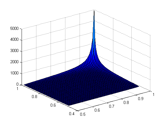
Figure 2. $(\alpha,\beta)\mapsto C_{1}(\alpha)C_{1}(\beta)$

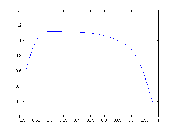
Figure 3. $\alpha\mapsto C_{2}(\alpha)$

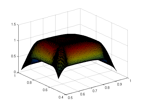
Figure 4. $(\alpha,\beta)\mapsto C_{2}(\alpha)C_{2}(\beta)$

References

- [1] P. Abry and V. Pipiras, Wavelet-based synthesis of the Rosenblatt process. Signal Process. 86 (2006) 2326–2339.
- [2] J. M. P. Albin, On extremal theory for self similar processes. Ann. Probab. 26 (1998) 743–793.
- [3] O. L. Banna and Y. S. Mishura, Approximation of fractional Brownian motion with associated hurst index separated from 1 by stochastic integral of linear power functions. Theor. Stoch. Proc. 30(2008) 1-16.
- [4] C. Chen, L. Sun and L. Yan, An approximation to the Rosenblatt process using martingale differences. Statist. Probab. Lett. 82 (2012) 748-757.
- [5] A. Chronopoulou, C. Tudor and F. Viens, Variations and Hurst index estimation for a Rosenblatt process using longer filters. Electron. J. Stat. 3 (2009) 1393-1435.
- [6] R. L. Dobrushin and P. Major, Non-central limit theorems for non-linear functionals of Gaussian fields. Z. Wahrscheinlichkeitstheorie verw. Gebiete. 50 (1979) 27-52.
- [7] J. Garzón, S. Torres and C. A. Tudor, A strong convergence to the Rosenblatt process, J. Math. Anal. Appl. 391 (2012), 630-647.
- [8] N. N. Leonenko and V. V. Ahn, Rate of convergence to the Rosenblatt distribution for additive functionals of stochastic processes with long-range dependence. J. Appl. Math. Stoch. Anal. 14 (2001) 27–46.
- [9] M. Maejima and C. A. Tudor, Wiener integrals with respect to the Hermite process and a non central limit theorem. Stoch. Anal. Appl. 25 (2007) 1043–1056.
- [10] M. Maejima and C. A. Tudor, Selfsimilar processes with stationary increments in the second Wiener chaos. Probab. Math. Statist. 32 (2012) 167–186.
- [11] M. Maejima and C. A. Tudor, On the distribution of the Rosenblatt process. Statist. Probab. Lett. 83 (2013) 1490–1495.
- [12] Y. S. Mishura and O. L. Banna, Approximation of fractional Brownian motion by wiener integrals. Theor. Probab. Math. Statist. 79(2009) 107-116.
- [13] V. Pipiras and M. S. Taqqu, Regularization and integral representations of Hermite processes. Statist. Probab. Lett. 80 (2010) 2014–2023.
- [14] G. Shen, X. Yin and D. Zhu, Weak convergence to the Rosenblatt sheet. Front. Math. China (2015) DOI:10.1007/s11464-015-0458-y.
- [15] N.-R. Shieh and Y. Xiao, Hausdorff and packing dimensions of the images of random fields. Bernoulli 16 (2010) 926-952.
- [16] M. Taqqu, Weak convergence to the fractional Brownian motion and to the Rosenblatt. Z. Wahrschein lichkeitstheor. Verwandte Geb. 31 (1975) 287-302.
- [17] M. Taqqu, Convergence of integrated processes of arbitrary Hermite rank. Z. Wahrscheinlichkeitstheorie verw. Gebiete 50 (1979) 53-83.
- [18] S. Torres and C. Tudor, Donsker type theorem for the Rosenblatt process and a binary market model. Stoch. Anal. Appl. 27 (2009) 555-573.
- [19] C. Tudor, Analysis of the Rosenblatt process. ESAIM Probab. Stat. 12 (2008) 230-257.
- [20] C. Tudor and F. Viens, Variations and estimators for the selfsimilarity order through Malliavin calculus. Ann. Probab. 37 (2009) 2093-2134.
- [21] C. Tudor, Analysis of Variations for Self-similar Processes. Berlin, Springer (2013).
- [22] L. Yan, Y. Li, and D. Wu, Appproximating the Rosenblatt process by multiple Wiener integrals. Electron. Commun. Probab. 20 (2015), 1-16.