Limit Theorems for Empirical Rényi Entropy and Divergence with Applications to Molecular Diversity Analysis

Abstract

Quantitative methods for studying biodiversity have been traditionally rooted in the classical theory of finite frequency tables analysis. However, with the help of modern experimental tools, like high throughput sequencing, we now begin to unlock the outstanding diversity of genomic data in plants and animals reflective of the long evolutionary history of our planet. This molecular data often defies the classical frequency/contingency tables assumptions and seems to require sparse tables with very large number of categories and highly unbalanced cell counts, e.g., following heavy tailed distributions (for instance, power laws). Motivated by the molecular diversity studies, we propose here a frequency-based framework for biodiversity analysis in the asymptotic regime where the number of categories grows with sample size (an infinite contingency table). Our approach is rooted in information theory and based on the Gaussian limit results for the effective number of species (the Hill numbers) and the empirical Renyi entropy and divergence. We argue that when applied to molecular biodiversity analysis our methods can properly account for the complicated data frequency patterns on one hand and the practical sample size limitations on the other. We illustrate this principle with two specific RNA sequencing examples: a comparative study of T-cell receptor populations and a validation of some preselected molecular hepatocellular carcinoma (HCC) markers.

keywords Hill number, Central limit theorem, Next generation sequencing, Triangular arrays, T-cell receptors

AMS classification 60F05 60G42 94A17

1 Introduction

Developing effective methods for quantifying and comparing empirical diversity of various biological populations is one of the fundamental problems of modern life sciences as it has direct impact on our understanding of the basic operating principles of our planet’s ecosystem and its evolution (cf., eg., Berkov et al, 2014). In the course of its 3.5 billion years of evolutionary history, nature has developed an outstanding bio- and molecular diversity among the Earth’s species of plants and animals. Indeed, it is estimated that there are currently about 8.7 million eukaryotic species on earth, both marine and terrestrial, 88% of which are still waiting to be described (Mora et al, 2011). The diversity at the molecular level is perhaps even more spectacular, as it occurs at different levels of biological organization: within one individual (e.g., through RNA, DNA, proteins, and metabolites), between individuals of the same and related species, within and between species and ecosystems, as well as throughout evolution (see, e.g., Campbell, 2003). For instance, the number of different molecular types of human T-cells is estimated at $10^{18}$ (Janeway, 2005) which only slightly less that the currently estimated number of stellar objects in the known universe (the latter believed to be of the order $10^{21}$).

Whereas the power of modern computing has allowed us to make steady progress towards building ever more robust empirical measures of biodiversity based on a variety of considerations (see, e.g., Presley et al, 2014), the most relevant to our discussion here are the measures borrowed from the field of information theory. They include among others the Hill number (or the effective number of species) and the related concept of the Renyi entropy (see, e.g., the recent review Chiu et al (2014) and references therein). Although originally proposed for quantifying ecological diversity in the macro-scale ecosystems (Chao et al, 2010), the use of the empirical Renyi entropy as a descriptor of diversity was also adopted for molecular populations in de Andrade and Wang (2011). Since then the Renyi-type measures were applied to problems of molecular populations ranging from analyzing regulatory variants and testing genome-wide associations (Sun and Hu, 2013; Sadee et al, 2014) to comparing different T-cell populations (Cebula et al, 2013; Rempala and Seweryn, 2013). Despite their growing usage in biodiversity studies of both macro- and molecular- level populations, it appears that some important statistical properties of the Renyi-type measures have not been yet sufficiently understood, especially in the context of frequency-based analysis and large sample behavior.

Currently, standard methods of obtaining molecular level data on the transcriptome (RNA) abundance rely on the so-called next-generation sequencing (NGS) technology and especially the high-throughput RNA sequencing or RNA-seq (Wang et al, 2009). However, the molecular count data from NGS often elude standard statistical analysis due to the fact that exhaustive sampling of the DNA and RNA fragments for the purpose of sequence reconstruction is not feasible and that the sequencing errors increase with sampling intensity or sequencing depth (O’Rawe et al, 2015). It has been therefore generally conceded (Oh et al, 2014) that the standard, fixed-dimension, non-parametric frequency/contingency table analysis (see, e.g., Agresti 2002) does not readily apply to the NGS data and that a different, infinite-size contingency table framework, more reflective of the current sequencing technology, appears necessary. Due to the nature of the NGS methods, such framework should be based on the large sample (high-throughput) considerations but, at the same time, should also account for the increase in the number of sequencing errors with increasing sample size as well as for the under-sampling bias.

Motivated by the questions on comparing biodiversity in molecular data (especially arriving from the NGS experiments) in the current paper we establish some large sample results for the empirical Renyi entropy and divergence in order to bridge the gap between current heuristic approaches and a more formal statistical theory of large samples. To this end, we derive herein several central limit theorems (CLTs) which yield approximate confidence bounds for the (Renyi) entropy-based measures of diversity and similarity in the setting of an infinite contingency table. Our CLT results complement both the law of large number theorems in Rempala and Seweryn (2013) as well as the CLT for the plugin estimates of the Shannon entropy Zhang and Zhang (2012) and the Kullback-Leibler divergence estimates (Paninski, 2003; Zhang and Grabchak, 2014). Since in the NGS experiments one typically expects to under-sample the transcriptome, we focus here on the Renyi entropy exponent (which below is denoted by $\alpha$) less than one, so as to up-weight the contributions of the lower counts and our CLT results are restricted to this case. The extensions to arbitrary exponents are straightforward but not considered here. In order to provide examples of the types of applications motivating the mathematical results, we analyze two real biological datasets from two different types of NGS experiments. In the first experiment, described in the study Cebula et al (2013), one compares multiple T-cell receptors populations taken from mice before and after treatment with antibiotics. The goal of the second experiment is the elucidation of differences in gene expression profiles between cancer and control tissues in individuals with hepatocellular carcinoma, as described in Chan et al (2014). In both presented examples the NGS datasets are analyzed and de-noised by applying a multi-stage process developed on the basis of our theoretical results.

As already indicated above, the problem of empirically estimating entropy and divergence has been extensively studied in the statistical and machine learning literature over past several decades, both in the context of discrete and continuous distributions. See, for instance, the monograph by Pardo (2005) or the review in Krishnamurthy et al (2014) for more details. In the general case of Renyi’s entropy and closely related Tsallis’ entropy of a fixed continuos distribution $f$ in ${\mathbb{R}}^{m}$, a class of consistent estimators was proposed in Leonenko et al (2008) based on the $k$-th nearest-neighbor distances computed from the appropriate random samples of size $n$ from $f$. The idea was later also extended to the Renyi entropy functionals in Källberg et al (2012) and it appears that similar results could be expected to hold in the discrete case as well. The main difference between these types of results and what is considered here is that in our setting the discrete density function $f$ is allowed to change as the sample size $n$ increases. Additionally, although in the current and that we only analyze the basic empirical frequency (the so-called plug-in) estimates.

The paper is organized as follows. In the next section (Section 2) we outline the relevant mathematical concepts along with the necessary notation. In Section 3 we state the main theoretical results of the paper, namely the CLTs for the Hill number (or the Tsallis entropy) and the Renyi entropy and divergence in the asymptotic regime when the diversity of the population (i.e., the number of different types) grows with the sample size. The results for the simpler case (Theorems 1 and 2) when Renyi entropy statistics admit linear approximations are established via the intermediate CLT results for the corresponding power sums which are closely related to the CLTs for Hill’s numbers and Tsallis’ entropies. These results are also included as parts of formulations of Theorems 1 and 2. In case of the uniform distribution for the Renyi entropy as well as the equal-marginals bivariate distribution for the Renyi divergence, the power sum CLTs are no longer valid (there is no linear approximation available) and other methods are required to establish weak convergence to Gaussian variates under slightly more stringent conditions. These results are presented as Theorems 3 and 4 in Section 3. As it turns out, the key ingredient needed to establish Theorems 3 and 4 is the CLT result for two Pearson-type chi-square statistics in an infinite contingency table. This latter result is of interest in itself and is presented as Lemma 2 in Section 3. In the following Section 4, we provide some simulation-based examples of the asymptotic behavior of estimates from Section 3 in the case (relevant for our applications) of power law distributions under various sampling scenarios. These examples illustrate in particular how the CLTs of Section 3 may hold or not, depending on the relations between the dimensions of the relevant contingency tables and the empirical sample sizes. In the second part of Section 4 we also discuss in detail the two biological examples of NGS data analysis and show how the results of Section 3 may be used to analyze biodiversity of T-cell receptors and to profile the multiple sets of transcriptomes. The final Section 5 offers a summary and brief conclusions. The proofs of all more complicated results are provided in the appendix along with some auxiliary technical lemmas.

2 Power Sums, Entropy and Divergence

Consider a triangular array of bivariate row-wise independent random variables $Z_{n,k}$ for $k=1,\ldots,n$ which in each row are equidistributed with the random variable $Z_{n}=(X_{n},Y_{n})$ such that $P(X_{n}=i,Y_{n}=j)=p_{ij}^{(n)}$ for $i,j=1,\ldots,m_{n}$. Below we suppress the index $n$ when possible, writing e.g., $m,Z_{k},Z,p_{ij}$, etc. for simplicity.

Let $\alpha>0$ and for any probability distribution ${\bm{p}}=(p_{i})_{i=1}^{m}$ define

$${\cal S}_{\alpha}({\bm{p}})=\sum_{i=1}^{m}{p}_{i}^{\alpha}.$$ (2.1)

Similarly, for any pair of distributions ${\bm{p}}=(p_{i})_{i=1}^{m}$ and ${\bm{q}}=(q_{i})_{i=1}^{m}$ define

$${\cal S}_{\alpha}({\bm{p}},{\bm{q}})=\sum_{i=1}^{m}{p}_{i}^{\alpha}q_{i}^{1-\alpha}.$$ (2.2)

(Note that ${\cal S}_{1}\equiv 1$). The well-known special case of the above is $\alpha=1/2$, which results in a symmetric index ${\cal S}_{1/2}({\bm{p}},{\bm{q}})={\cal S}_{1/2}({\bm{q}},{\bm{p}})$ often referred to as the Bhattacharyya coefficient (see, e.g., Nielsen and Boltz, 2011).

Recall (Renyi, 1961) that for a given distribution ${\bm{p}}$ its Renyi entropy $\mathcal{H}_{\alpha}$ is defined as

$$\mathcal{H}_{\alpha}({\bm{p}})=\frac{1}{1-\alpha}\log\left(\sum p_{i}^{\alpha}\right)=\frac{1}{1-\alpha}\log{\cal S}_{\alpha}({\bm{p}})$$

and that for a pair of distributions $({\bm{p}},{\bm{q}})$ their Renyi divergence $\mathcal{D}_{\alpha}$ is defined as

$$\mathcal{D}_{\alpha}({\bm{p}},{\bm{q}})=\frac{1}{\alpha-1}\log{\cal S}_{\alpha}({\bm{p}},{\bm{q}}).$$

Note that the sign change in the normalizing constant is needed in order to ensure non-negativity of $\mathcal{H}_{\alpha}$ and $\mathcal{D}_{\alpha}$. The special case of $\mathcal{D}_{\alpha}$ with $\alpha=1/2$ is referred to as the Bhattacharyya distance, and may be expressed in terms of the Mahalanobis distance (see, e.g., Nielsen and Boltz, 2011), whereas the linear approximation of $\mathcal{H}_{\alpha}({\bm{p}})$ given by

$$\mathcal{T}({\bm{p}})=\frac{1}{1-\alpha}({\cal S}_{\alpha}({\bm{p}})-1).$$ (2.3)

is sometimes referred to as the Tsallis entropy and has important applications in the field of statistical mechanics (Tsallis, 1988). Note that for our current purposes, we will only consider the quantities $\mathcal{D}_{\alpha},\mathcal{H}_{\alpha}$, and $\mathcal{T}$ for $\alpha$ satisfying $0<\alpha<1$.

In what follows the summation symbol without subscripts ($\sum$) will indicate summation with respect to the index $i$ ($i=1,\ldots,m$) whereas ${\bm{p}}=(p_{i})_{i=1}^{m}$ and ${\bm{q}}=(q_{i})_{i=1}^{m}$ will (typically) denote the marginal distributions of the bivariate variable $Z=(X,Y)$ whose distribution is denoted by $(p_{ij})_{i,j=1}^{m}$. Additionally, the uniform distribution on $m$ points will be denoted by ${\bm{u}}$. An important relation between the Renyi entropy and the Renyi divergence is

$$\mathcal{H}_{\alpha}({\bm{p}})=\log m-\mathcal{D}_{\alpha}({\bm{p}},{\bm{u}}).$$ (2.4)

We note also the following monotonicity property of $\mathcal{D}_{\alpha}$ and $\mathcal{H}_{\alpha}$ with respect to the index $\alpha$.

Lemma 1.

For $0<\alpha<\beta<1$ we have $\mathcal{D}_{\alpha}({\bm{p}},{\bm{q}})\leq{\cal D}_{\beta}({\bm{p}},{\bm{q}})$ and thus, in view of (2.4), also $\mathcal{H}_{\alpha}({\bm{p}})\geq{\cal H}_{\beta}({\bm{p}})$.

Proof.

Note that for $x\geq 0$ the function $x\rightarrow x^{\frac{\alpha-1}{\beta-1}}$ is strictly convex for $0<\alpha<\beta<1$. Therefore, by Jensen’s inequality

$$\mathcal{D}_{\alpha}({\bm{p}},{\bm{q}}) =\frac{1}{\alpha-1}\log\sum p_{i}^{\alpha}q_{i}^{1-\alpha}=\frac{1}{\alpha-1}\log\sum p_{i}\left(\frac{q_{i}}{p_{i}}\right)^{(1-\beta)\frac{\alpha-1}{\beta-1}}$$

$$\leq\frac{1}{\beta-1}\log\sum p_{i}\left(\frac{q_{i}}{p_{i}}\right)^{(1-\beta)}={\cal D}_{\beta}({\bm{p}},{\bm{q}}).$$

∎

Example 2.1 (Hill’s Number).

For given $0<\alpha<1$ the measure of diversity of a distribution ${\bm{p}}$ also known as the effective number of classes may be defined as (see, e.g., Jost, 2007; Chao et al, 2012; Rempala and Seweryn, 2013) $ENC_{\alpha}({\bm{p}})=\exp(\mathcal{H}_{\alpha}({\bm{p}}))={\cal S}_{\alpha}({\bm{p}})^{1/(1-\alpha)}$. It follows then from Lemma 1 that for any $0<\alpha<\beta<1$ we have $ENC_{\alpha}({\bm{p}})\geq ENC_{\beta}({\bm{p}})$. (As it turns out, this inequality may be in fact extended to arbitrary positive $\alpha<\beta$).

2.1 Low Diversity Condition and Projection Variables

The notion of an infinite-dimension contingency table brought up in the introduction may be now formally introduced simply as a requirement that for $n$-size sample from $(p_{ij})_{i,j=1}^{m}$ we have $m\to\infty$ as $n\to\infty$. Throughout the paper, let $a\wedge b$ denote $\min(a,b)$ for any real $a,b$ and let $a_{n}\sim b_{n}$ (resp. $a_{n}\sim O(b_{n})$) denote $a_{n}/b_{n}\to 1$ (resp. $A<\limsup_{n}a_{n}/b_{n}<B$ for some finite $A,B$) as $n\to\infty$ for any real sequences $a_{n},b_{n}$. Throughout the paper we consider only the low diversity (LD) schemes in which the marginals ${\bm{p}},{\bm{q}}$, of $Z$ satisfy the following LD condition.

$$(np_{\ast})^{-1}=o(n^{-\tau})\quad\text{for some}\quad\tau>0,$$ (2.5)

where $p_{\ast}=\min_{i}(p_{i})\wedge\min_{i}(q_{i})$. Note that since $p_{\ast}\leq 1/m$ then (2.5) implies in particular $m/n=o(n^{-\tau})$. As it turns out, for many distributions ${\bm{p}}$ the two conditions are in fact equivalent, as seen in the following.

Example 2.2 (Power Law Model).

Let ${\bm{p}}={\bm{q}}$ and assume that $p_{i}=H^{-1}(\beta,m)/(i^{\beta}l(i))$, $(i=1,\ldots,m)$ where $\beta>0$, $l(x)$ is a non-decreasing slowly varying function (see, e.g., Soulier 2009, chapter 1), and $H^{-1}(\beta,m)=1/\sum_{i=1}^{m}({i^{\beta}l(i)})^{-1}$ is the normalizing constant. Note that if $0<\beta<1$ then $H^{-1}(\beta,m)\sim(1-\beta)l(m)/m^{1-\beta}$ and (2.5) is implied by $m/n=o(n^{-\tau})$ since

$$(n\min_{i}p_{i})^{-1}\sim(1-\beta)^{-1}\frac{m^{\beta}l(m)}{nm^{\beta-1}l(m)}=(1-\beta)^{-1}\frac{m}{n}.$$

For any $0<\alpha<1$ and a given pair $(m,n)$, let us define two random variables which will play an important role in the following section. Let $W_{n}^{(\alpha)}$ be defined as

$$P(W_{n}^{(\alpha)}=\alpha p_{i}^{\alpha-1})=p_{i}$$ (2.6)

for $i=1,\ldots,m$. Similarly, define also $V_{n}^{(\alpha)}$ as

$$P\left(V_{n}^{(\alpha)}=\alpha\left(\frac{q_{i}}{p_{i}}\right)^{1-\alpha}+(1-\alpha)\left(\frac{p_{j}}{q_{j}}\right)^{\alpha}\right)=p_{ij}$$ (2.7)

for $i,j=1,\ldots,m$. In the following, for the reasons discussed below, we refer to (2.6) and (2.7) as the projection variables or simply projections.

Remark 2.1.

Note that

$$EW_{n}^{(\alpha)}=\alpha{\cal S}_{\alpha}({\bm{p}})$$

and $VarW_{n}^{(\alpha)}=0$ iff $p_{i}=1/m$ for all $i$, that is, ${\bm{p}}=(p_{i})={\bm{u}}$ is a uniform distribution on $m$ support points (this case is often referred to as a maximal diversity model or a pure noise model). Similarly,

$$EV_{n}^{(\alpha)}={\cal S}_{\alpha}({\bm{p}},{\bm{q}})$$

and it is also easy to see that $VarV_{n}^{(\alpha)}=0$ iff $p_{i}=q_{i}$ for all $i$, that is, ${\bm{p}}={\bm{q}}$.

As it turns out, both cases ${\bm{p}}={\bm{u}}$ and ${\bm{p}}={\bm{q}}$ require special consideration in the asymptotic analysis of $\mathcal{H}_{\alpha}$ and $\mathcal{D}_{\alpha}$. In view of the remark above they may be referred to as the cases of “degenerate” (zero variance) projections.

Example 2.3 (Noise–and–Signal and Pure Noise Models).

A distribution concentrated on $m+1$ support points, such that $p_{0}>0$ and $p_{i}=(1-p_{0})/m$ for $1\leq i\leq m$, may be considered as a simple model of signal contamination. Note that in this case we have $P(W_{n}^{(\alpha)}=\alpha p_{0}^{\alpha-1})=p_{0}$, $P(W_{n}^{(\alpha)}=\alpha m^{1-\alpha}(1-p_{0})^{\alpha-1})=1-p_{0}$ and

$$VarW_{n}^{(\alpha)}=\alpha^{2}\left(m^{1-\alpha}(1-p_{0})^{\alpha}\left(\frac{p_{0}}{1-p_{0}}\right)^{1/2}-p_{0}^{\alpha}\left(\frac{1-p_{0}}{p_{0}}\right)^{1/2}\right)^{2}.$$

For the pure noise model $p_{0}=0$, in which case the support reduces to $m$ points, and the above formula is not valid. However, as already pointed out before, in this case we may show directly that $VarW_{n}^{(\alpha)}=0$.

3 Limit Theorems

Let $N(0,1)$ denote the standard Gaussian random variable and $\Rightarrow$ denote the usual weak convergence in the space of probability distributions. Define also the plug-in $n$-sample estimates of ${\bm{p}}$ and ${\bm{q}}$ as, respectively, $\hat{\bm{p}}=(\hat{p}_{i})_{i=1}^{m},$ where $\hat{p}_{i}=\sum_{k=1}^{n}I(X_{k}=i)/n$ and $\hat{{\bm{q}}}=(\hat{q}_{i})_{i=1}^{m},$ where $\hat{q}_{i}=\sum_{k=1}^{n}I(Y_{k}=i)/n$. Here and elsewhere in the paper $I(\cdot)$ denotes the indicator function. As it turns out, two distinct sets of CLTs may be derived depending on whether the variables $W_{n}^{(\alpha)}$ and $V_{n}^{(\alpha)}$ are degenerate (that is, their respective variances vanish) or not. For the non-degenerate case the appropriate CLTs may be established by expanding on the usual projection and Taylor’s expansion arguments (see, e.g., Shao, 2003, chapter 1). This is the simpler case to consider and we discuss it first.

3.1 CLTs for Non-Degenerate Projections

The first two CLT results for the empirical (plug-in) Renyi entropy and divergence and their corresponding power sums are provided in Theorems 1 and 2 below. Their respective hypotheses $(iii)$ may be viewed as complementing the analogous results established for the Shannon entropy and the Kullback-Leibler divergence (Paninski, 2003; Zhang and Zhang, 2012; Zhang and Grabchak, 2014). Note also that ${\cal S}_{\alpha}=(ENC_{\alpha})^{1-\alpha}$ where the Hill number $ENC_{\alpha}$ is defined in Example 1. The proofs are deferred to the appendix.

Recall that for any square integrable random variable $X$, such that $EX\neq 0$, we define its coefficient of variation as ${\cal CV}(X)=(VarX)^{1/2}|EX|^{-1}$.

Theorem 1 (Renyi Entropy CLT).

Let $W_{n}^{(\alpha)}$ be a sequence of random variables defined by (2.6) with $\inf_{n}\mathcal{CV}(W_{n}^{(\alpha)})>0$ and let

$$\sum p_{i}^{\alpha-1}(nVarW_{n}^{(\alpha)})^{-1/2}\to 0\quad\text{for}\ m,n\to\infty.$$ (3.1)

Then, under the LD condition (2.5), as $m,n\to\infty$

• ${\cal S}_{\alpha}(\hat{\bm{p}})/{\cal S}_{\alpha}({\bm{p}})\to 1$ in probability,

• $\sqrt{n}({\cal S}_{\alpha}(\hat{\bm{p}})-{\cal S}_{\alpha}({\bm{p}}))/(VarW_{n}^{(\alpha)})^{1/2}\Rightarrow N(0,1),$

• $\sqrt{n}\,(1/\alpha-1)(\mathcal{H}_{\alpha}(\hat{\bm{p}})-\mathcal{H}_{\alpha}({\bm{p}}))/\mathcal{CV}(W_{n}^{(\alpha)})\Rightarrow N(0,1).$

Remark 3.1.

Note that the first two assertions of the theorem may be equivalently stated in terms of the convergence of the Tsallis plug-in entropy defined by (2.3).

Remark 3.2.

Note that the condition (3.1) is typically stronger than (2.5). Indeed, taking $\alpha>1/2$ and the power law model from Example 2 with $0<\beta<1$ we obtain $\sum p_{i}^{\alpha}\sim(1-\beta)^{\alpha}\,m^{1-\alpha}/(1-\alpha\beta)$ and $\sum p_{i}^{2\alpha-1}\sim(1-\beta)^{2\alpha-1}\,m^{2-2\alpha}/(1-2\alpha\beta+\beta)$. Consequently, for some constant $C>1$

$$\frac{C\sum p_{i}^{\alpha-1}}{\sqrt{n(\sum p_{i}^{2\alpha-1}-(\sum p_{i}^{\alpha})^{2})}}\geq\frac{m}{\sqrt{n}}\frac{(\max_{i}p_{i})^{\alpha-1}}{m^{1-\alpha}}\geq\frac{m}{\sqrt{n}}$$

for large $m,n$ and (3.1) implies (2.5) with $\tau=1/2$. Similarly, (possibly for different $C>1$)

$$\frac{\sum p_{i}^{\alpha-1}}{\sqrt{n(\sum p_{i}^{2\alpha-1}-(\sum p_{i}^{\alpha})^{2})}}\leq\frac{Cm}{\sqrt{n}}\frac{(\min_{i}p_{i})^{\alpha-1}}{m^{1-\alpha}}\leq C\frac{m}{\sqrt{n}}$$

and therefore in this case (3.1) is seen to be actually equivalent to (2.5) with $\tau=1/2$.

Remark 3.3 (Plug-in Bias).

Note that, in view of Jensen’s inequality applied to the strictly concave function $x\rightarrow x^{\alpha}$ for $x>0$ and $0<\alpha<1$, we have $E{\cal S}_{\alpha}(\hat{\bm{p}})/{\cal S}_{\alpha}({\bm{p}})\leq 1$. This and the assertion $(i)$ above imply together that under the assumptions of Theorem 1 the relative bias of ${\cal S}_{\alpha}(\hat{\bm{p}})$ satisfies $E{\cal S}_{\alpha}(\hat{\bm{p}})/{\cal S}_{\alpha}({\bm{p}})-1\to~{}0$ as $n,m\to\infty$. The standard inequality $\log x\leq x-1$ valid for $x>0$ implies then that the bias of the plug-in entropy estimate satisfies

$$E\mathcal{H}_{\alpha}(\hat{\bm{p}})-\mathcal{H}_{\alpha}({\bm{p}})\to 0\qquad\text{as}\quad n,m\to\infty.$$ (3.2)

Unfortunately, as may be seen from the proof of Theorem 1 in the appendix, a more careful analysis of the tail events for the plug-in estimate than the one currently performed is needed in order to actually establish a convergence rate in (3.2).

Turning now to our second result, note that the relation (2.4) suggests that CLT of Theorem 1 could be also extended to the Renyi divergence. The proof is again based on the Taylor expansion method where now the projection variable (2.6) is replaced by (2.7).

Theorem 2 (Renyi Divergence CLT).

Let $V_{n}^{(\alpha)}$ be a sequence of random variables defined by (2.7) with $\inf_{n}\mathcal{CV}(V_{n}^{(\alpha)})>0$ and let

$$\left(\sum\left({q_{i}}/{p_{i}}\right)^{1-\alpha}+\sum\left({p_{i}}/{q_{i}}\right)^{\alpha}\right)(nVarV_{n}^{(\alpha)})^{-1/2}\to 0\quad\text{for}\ m,n\to\infty.$$ (3.3)

Then, under the LD condition (2.5), as $m,n\to\infty$

• $\displaystyle{{\cal S}_{\alpha}(\hat{\bm{p}},\hat{{\bm{q}}})/{\cal S}_{\alpha}({\bm{p}},{\bm{q}})\to 1}$ in probability,

• $\displaystyle{\sqrt{n}({\cal S}_{\alpha}(\hat{\bm{p}},\hat{{\bm{q}}})-{\cal S}_{\alpha}({\bm{p}},{\bm{q}}))/(VarV_{n}^{(\alpha)})^{1/2}\Rightarrow N(0,1)},$

• $\displaystyle{\sqrt{n}\,(\alpha-1)(\mathcal{D}_{\alpha}(\hat{\bm{p}},\hat{{\bm{q}}})-\mathcal{D}_{\alpha}({\bm{p}},{\bm{q}}))/\mathcal{CV}(V_{n}^{(\alpha)})\Rightarrow N(0,1).}$

Remark 3.4 (Plug-in Bias).

Note that, similarly as in Remark 3.3, we have $E{\cal S}_{\alpha}(\hat{\bm{p}},\hat{{\bm{q}}})/{\cal S}_{\alpha}({\bm{p}},{\bm{q}})\leq 1$ and, by a similar argument as before, Theorem 2$(i)$ implies

$$E\mathcal{D}_{\alpha}(\hat{\bm{p}},\hat{{\bm{q}}})-\mathcal{D}_{\alpha}({\bm{p}},{\bm{q}})\to~{}0\qquad\text{as}\ n,m\to\infty.$$

Example 3.1 (Symmetric Divergence for Power Laws).

Consider the symmetric divergence ${\cal D}_{1/2}({\bm{p}},{\bm{q}})$ with independent marginals, which often is the case of interest in NGS applications. Note that in this situation $VarV_{n}^{(1/2)}=1/2-(\sum\sqrt{p_{i}q_{i}})^{2}/2$. Suppose additionally that $p_{i}=H^{-1}(\beta_{1},m)/(i^{\beta_{1}}l_{1}(i))$ and $q_{i}=H^{-1}(\beta_{2},m)/(i^{\beta_{2}}l_{2}(i))$, $(i=1,\ldots,m)$ where the notation is as in Example 2 with $0<\beta_{1}\neq\beta_{2}<1$. Then

$$VarV_{n}^{(1/2)}\sim\frac{1}{2}-\frac{\sqrt{(1-\beta_{1})(1-\beta_{2})}}{2-\beta_{1}-\beta_{2}}$$

and, consequently, (3.3) is seen as equivalent to $m/\sqrt{n}\to 0$ (cf. also Remark 3.2 above).

With some additional effort, the two CLT results of this section may be extended to degenerate projections. This is discussed in the next section.

3.2 CLTs for Degenerate Projections

In case of a degenerate projection, the linear term of the power sum Taylor’s expansion disappears (cf. formula (B.6) in the appendix) and the condition (3.1) is no longer needed. However, the LD assumption (2.5) has to be slightly strengthened in order to establish the asymptotic results for the leading (quadratic) term of the appropriate expansion.

3.2.1 Chi-Square Statistic CLT

The following lemma describing the chi-square statistic CLT may be of independent interest for models of sparse contingency tables. For a recent discussion of a normal approximation to the chi-square statistic in such settings, see, e.g., Horgan and Murphy (2013). Here we apply the chi-square CLT formulated below to obtain weak limits for the quadratic terms in the entropy and divergence Taylor’s expansions leading to Theorems 3 and 4 described in the next subsection. To begin, consider a pair of distributions $({\bm{p}},{\bm{q}})$ and a set of positive weights ${\bm{r}}=(r_{i})_{i=1}^{m}$ and define the corresponding chi-square ($\chi^{2}$) distance function as

$${\cal X}^{2}_{\bm{r}}({\bm{p}},{\bm{q}})=n\sum\frac{(p_{i}-q_{i})^{2}}{r_{i}}.$$

Note that, for instance, the $\chi^{2}$-distance statistic between the empirical marginals $(\hat{\bm{p}},\hat{{\bm{q}}})$ is obtained by setting $r_{i}=p_{i}+q_{i}$

$${\cal X}^{2}_{\bm{r}}(\hat{\bm{p}},\hat{{\bm{q}}})=n\sum\frac{(\hat{p}_{i}-\hat{q}_{i})^{2}}{p_{i}+q_{i}}$$

and the Pearson $\chi^{2}$-statistic is obtained by setting $r_{i}=p_{i}$

$${\cal X}^{2}_{\bm{p}}(\hat{\bm{p}},{\bm{p}})=n\sum\frac{(\hat{p}_{i}-p_{i})^{2}}{p_{i}}.$$ (3.4)

Below we denote ${\cal X}^{2}_{\bm{u}}(\hat{\bm{u}},{\bm{u}})=:{\cal X}^{2}_{\bm{u}}$.

Lemma 2.

Let $(p_{ij})_{i,j=1}^{m}$ be the bivariate distribution of $Z=(X,Y)$ with $X$ and $Y$ having marginals $(p_{i})_{i=1}^{m}$ and $(q_{i})_{i=1}^{m}$ where $p_{i}=q_{i}>0$. Assume $m\to\infty$ as $n\to\infty$ and

$$(mn)^{-1}\sum\max(p_{i}^{-1},p_{i}^{-2}m^{-1})\to 0,$$ (3.5)

Then as $n\to\infty$

• $\displaystyle{\frac{{\cal X}^{2}_{\bm{p}}(\hat{\bm{p}},{\bm{p}})-m}{\sqrt{2m}}\Rightarrow N(0,1)},$
  and if additionally

  $$\sup_{n}\max_{ij}\frac{p_{ij}}{p_{i}p_{j}}=B<\infty$$ (3.6)

  then also

• $\displaystyle{\frac{{\cal X}^{2}_{2{\bm{p}}}(\hat{\bm{p}},\hat{{\bm{q}}})-\mu_{n}}{\sqrt{2}\gamma_{n}}\Rightarrow N(0,1)},$
  where

  $$\mu_{n} =\sum_{i}(1-p_{ii}/p_{i})$$

  $$\gamma_{n}^{2} =\sum_{i}\frac{(p_{i}-p_{ii})^{2}}{p_{i}^{2}}+\sum_{1\leq i\neq j\leq m}\frac{(p_{ij}+p_{ji})^{2}}{4p_{i}p_{j}}.$$ (3.7)

Remark 3.5.

Note that for ${\cal X}_{{\bm{u}}}^{2}$ the condition (3.5) simplifies to $m/n\to 0$.

Remark 3.6.

Note that under the assumption (3.6) we have $m-2B\leq\gamma_{n}^{2}\leq m+B^{2}$ and therefore $\gamma_{n}^{2}\sim m$. In particular, if $p_{ij}=p_{i}p_{j}$ then $\mu_{n}=\gamma_{n}^{2}=m-1$.

The proof of the result may be found in the appendix. Its application is discussed next.

3.2.2 Pure Noise and Equal Marginals CLTs

The first result covers the case of Renyi entropy when ${\bm{p}}={\bm{u}}$. The proof is outlined in the appendix. Recall that for real $a$ and integer $k$ we define $\binom{a}{k}=a(a-1)\cdots(a-k+1)/k!$

Theorem 3 (Uniform Entropy CLT).

Assume $m\to\infty$ as $n\to\infty$ and $m^{2}/n=o(n^{-\tau})$ for $\tau>0$. Then

• $\frac{n\binom{\alpha}{2}^{-1}[m^{\alpha-1}{\cal S}_{\alpha}(\hat{\bm{u}})-1]-m}{\sqrt{2m}}\Rightarrow N(0,1)$

• $\frac{n[\mathcal{H}_{\alpha}(\hat{\bm{u}})-\log m-(1-\alpha)^{-1}{\log(1+\binom{\alpha}{2}\frac{m}{n}})]}{\alpha\sqrt{m/2}}\Rightarrow N(0,1).$

Our second CLT result is the following theorem for Renyi divergence when ${\bm{p}}={\bm{q}}$. The proof is again deferred to the appendix.

Theorem 4 (Degenerate Divergence CLT).

Let $(p_{ij})_{i,j=1}^{m}$ be the bivariate distribution of $Z=(X,Y)$ with $X$ and $Y$ having marginals ${\bm{p}}=(p_{i})_{i=1}^{m}$ and ${\bm{q}}=(q_{i})_{i=1}^{m}$ where $p_{i}=q_{i}>0$. Let $\mu_{n}$ and $\gamma_{n}^{2}$ be given by (3.7). Assume $m\to\infty$ as $n\to\infty$ and that (3.6) holds, as well as that

$$\max\left\{\frac{1}{nm\min p_{i}^{2}},\frac{m}{n\min p_{i}}\right\}=o(n^{-\tau}).$$ (3.8)

Then

• $\frac{n(\alpha(\alpha-1))^{-1}[{\cal S}_{\alpha}(\hat{\bm{p}},\hat{{\bm{q}}})-1]-\mu_{n}}{\sqrt{2}\gamma_{n}}\Rightarrow N(0,1)$

• $\frac{n[\mathcal{D}_{\alpha}(\hat{\bm{p}},\hat{{\bm{q}}})-(\alpha-1)^{-1}\log(1+\alpha(\alpha-1)\frac{\mu_{n}}{n})]}{\alpha\sqrt{2}\gamma_{n}}\Rightarrow N(0,1).$

Remark 3.7.

Note that for ${\bm{p}}={\bm{q}}={\bm{u}}$ the condition (3.8) reduces to $m^{2}/n=o(n^{-\tau})$ required in Theorem 3.

3.2.3 Random Sample Size

When analyzing NGS data some part of the sequences reads is frequently removed for technical reasons, for instance, due to poor amplification or reading errors (see next section). In such cases one effectively deals with a molecular sample of random size. Our CLT results derived earlier may be extended to this case as well, with the help of following simple result described in Theorem 5 below. Its various versions have been discussed, for instance, in the context of random allocations (see, e.g., Kolchin et al, 1978).

Theorem 5 (Randomized Sample CLT).

Let $(Z_{n})_{n=1}^{\infty}$ be a sequence of bivariate variables supported on an $m_{n}\times m_{n}$ integer lattice with distribution $(p_{ij})_{i,j=1}^{m_{n}}$. Let $(\hat{Z}_{n})=(\hat{p}_{ij})_{i,j=1}^{m_{n}}$ $(n=1,2,3,\ldots,)$ be the sequence of the empirical estimates, each based on an iid sample of (deterministic) size $n$. Suppose that the statistic ${\cal G}_{n}={\cal G}_{n}(\hat{p}_{ij})$ satisfies $b_{n}({\cal G}_{n}-a_{n})\Rightarrow N(0,1)$ as $n\to\infty$ with some non-random $(a_{n},b_{n})$. Let $(\nu_{n})_{n=1}^{\infty}$ be a sequence of random variables independent of $(\hat{Z}_{n})_{n=1}^{\infty}$ and following the binomial distributions $bin(n,\tau_{n})$ with $0<\inf_{n}\tau_{n}\leq\sup_{n}\tau_{n}<1$. Then also

$$b_{\nu_{n}}({\cal G}_{\nu_{n}}-a_{\nu_{n}})\Rightarrow N(0,1).$$

Proof.

Denote by ${\cal G}_{n_{k}}$ the random variable ${\cal G}_{\nu_{k}}$ conditional on the event $\nu_{k}=n_{k}$ and by $\Phi$ the distribution function of the standard normal random variable. By assumption, for any real $x$ we have $P({\cal G}_{n_{k}}\leq x)\to\Phi(x)$ provided that $n_{k}\to\infty$ as $k\to\infty$. Let $\varepsilon>0$ be sufficiently small and define $C_{\varepsilon}(k_{0})=\{n_{k}:k(\tau_{k}-\varepsilon)\leq n_{k}\leq k(\tau_{k}+\varepsilon),k>k_{0}\}$. Note that by the weak law of large numbers $P(\nu_{k}\in C_{\varepsilon}(k_{0}))\to 1$ as $k_{0}\to\infty$. Therefore

$$P({\cal G}_{\nu_{k}}\leq x,\nu_{k}\in C_{\varepsilon}(k_{0})) =\sum_{n_{k}\in C_{\varepsilon}(k_{0})}P({\cal G}_{n_{k}}\leq x)P(\nu_{k}=n_{k})$$

$$=(\Phi(x)+\delta(k_{0}))P(\nu_{k}\in C_{\varepsilon}(k_{0}))$$

where $\delta(k_{0})\to 0$ as $k_{0}\to\infty$. Accordingly, as $k_{0}\to\infty$ the left-hand side converges to $\lim_{k}P({\cal G}_{\nu_{k}}\leq x)$ and the right-hand side to $\Phi(x)$ and the result follows. ∎

4 Examples and NGS Applications

We start by providing some numerical examples illustrating that, in general, the CLT results discussed above do not hold without assumptions on the relative rate of $m$ and $n$. Next, we show two examples of applicability of our results to analyzing biodiversity of NGS data. The first one is concerned with comparing the diversity of T-cell receptor populations in transgenics mice, whereas the second one aims at identifying the hepatocellular carcinoma transcription profiles in humans. For the purpose of the T-cell receptors example, we propose a sequential statistical procedure of NGS signal filtering based on our CLT results from the previous sections. We begin by pointing out to some subtleties in the CLT results discussed in Section 3.

4.1 Power Law and Pure Noise Models

Consider the power law model from Example 2 in Section 2.1 with $\beta=1$ and $l(x)\equiv 1$. Note that in this case $(n\min_{i}p_{i})^{-1}\sim m\log m/\,n$ as well as $\sum p_{i}^{\alpha-1}(nVarW_{n}^{(\alpha)})^{-1/2}\sim O(m(\log^{2\alpha}m/n)^{1/2})$ and therefore the assumptions of Theorem 1 are satisfied as soon as

$$n^{\tau-1}m\to 0$$ (4.1)

for some $\tau>1/2$. Similarly, the assumption (3.5) of Lemma 2 is satisfied as soon as

$$\log^{2}\!m\,\frac{m}{n}\to 0.$$ (4.2)

In Figure 1 we illustrate the convergence results of Theorem 1$(iii)$ and Lemma 2$(i)$ for this power law model and $\alpha=0.5$. The panels of Figure 1 presents the sample vs standard normal quantile (QQ) plots for the normalized Renyi entropy statistic and the normalized Pearson statistic (3.4) based on $B=5000$ samples from the power law distribution, each with $m=1000$ and three different values of $n=m^{1+\varepsilon}$ ($\varepsilon=-0.5,0.5,1.5$). As seen from the plots, in the absence of (4.1) the CLT result for the Renyi entropy (cf. Theorem 1$(iii)$) does not hold. Moreover, the middle panel QQ plot indicates that for large $m,n$ satisfying $n=m^{3/2}$ the discrepancy between distribution of the entropy function and its plug-in estimate appears in a form of deterministic shift, indicating the presence of substantial asymptotic bias and hence the lack of convergence (3.2). Similarly, when (4.2) is not satisfied than the Pearson statistic CLT given in Lemma 2$(i)$ fails with the middle panel again indicating that the bias of the estimate does not vanish when $m$ is too large relative to $n$.

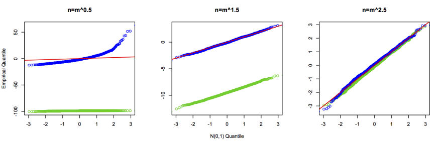
Figure 1: Projection CLTs. Normal QQ plots for the normalized Renyi entropy (Theorem 1$(iii)$, lower (green) curve) and normalized Pearson $\chi^{2}$ statistic (Lemma 2$(i)$, upper (blue) curve) for the power law distribution $p_{i}=1/i$. The panels shows quantile plots with different values of $n=m^{1+\varepsilon}$ ($\varepsilon=-0.5,0.5,1.5$) and $m=1000$. The solid (red) line gives quantiles of the standard normal distribution for reference.

For comparison, we also considered the uniform distribution (pure noise) model $p_{i}=1/m$. Note that it may be viewed as a degenerate power law where $\beta=0$ and $l(x)\equiv 1$. Recall that according to Theorem 3 $(ii)$ and Lemma 2 $(i)$, the sufficient conditions for the respective CLTs are $m^{2}/n^{1-\tau}\to 0$ and $m/n\to 0$ (see Remark 3.5 for the latter one). The necessity of these conditions is illustrated in the panels of Figure 2 where we again present the (normal) QQ plots for the Renyi ($\alpha=0.5$) and the Pearson statistics for the same values of $B,n$ and $m$ as in Figure 1. As seen from these plots, only in the last panel, when $m^{2}/n\approx 0$, we get good CLT approximation for both statistics. These results appear consistent with our theoretical results from Theorem 3 and Lemma 2.

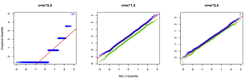
Figure 2: Degenerate Projection CLTs. Normal QQ plots for the normalized uniform Renyi entropy (Theorem 3$(ii)$, represented by the lower (green) curve) and the normalized Pearson $\chi^{2}$-statistic (Lemma 2 $(i)$, represented by the upper (blue) curve) with $p_{i}=m^{-1}$. The panels shows quantile plots with different values of $n=m^{1+\varepsilon}$ ($\varepsilon=-0.5,0.5,1.5$) and $m=1000$. The solid (red) line gives the quantiles of the standard normal distribution for reference. Note that the normalized Renyi entropy is undefined for the first panel.

Although not presented here due to space considerations, similar examples based on the bivariate power laws may be used to illustrate the necessity of the assumptions of type (3.3) and (3.8) in the CLT results for divergence in Theorems 2$(iii)$ and 4$(ii)$.

4.2 Applications to NGS Data

Our CLT results described in Section 3 were originally motivated by questions rising in NGS data analysis. Below we describe two examples which adhere to the following basic framework. Denote by $\bm{\varepsilon}_{1},\bm{\varepsilon}_{2}$ two independent noise distributions each on $m$ support points, and assume that a pair $({\bm{p}},{\bm{q}})$ of marginal distributions may be represented as

$$({\bm{p}},{\bm{q}})=\lambda(\tilde{\bm{p}},\tilde{\bm{q}})+(1-\lambda)(\bm{\varepsilon}_{1},\bm{\varepsilon}_{2})$$ (4.3)

where $(\tilde{\bm{p}},\tilde{\bm{q}})$ is a pair of marginal distributions having no common support points with $(\bm{\varepsilon}_{1},\bm{\varepsilon}_{2})$ and $\lambda$ is the mixing proportion (or prior probability of signal). We assume that each $\bm{\varepsilon}$ is a simple finite mixture of $K$ uniform distributions on separate support. Note that the noise-and-signal model from Example 2.3 in Section 2.1 may be viewed as a (univariate) special case of (4.3) with $K=1$. In the first example below we took $K=2$.

	Antibiotic ($\tilde{\bm{p}}$)	Control ($\tilde{\bm{q}}$)
$n$	39,084	39,084
$m$	165	165
$k_{m}$	17	17
$\hat{\lambda}$	0.46	0.46
$\hat{\beta}$	0.869(0.05)	0.971(0.05)
${\cal H}_{1/2}$	4.81 (4.79, 4.82)	4.64 (4.63, 4.67)
$ENC_{1/2}$	122.73 (120.30, 123.97)	103.54 (102.51, 106.70)
${\cal D}_{1/2}$	0.155 (0.147, 0.163)

Table 1: Results of TCR data analysis. The mixture model (4.3) with heavy-tailed power laws fitted to two sets of TCR counts derived from mouse MLN before and after an antibiotic treatment as described in Cebula et al (2013). The empirical Renyi entropy, the Hill number and the Renyi diversity CIs (in parenthesis) are obtained from the CLT results of Theorems 1 and 2.

Algorithm 1(NGS Diversity Analysis with $\mathcal{D}_{\alpha}$ or ${\cal S}_{\alpha}$)  

• Exponent ($\alpha$) selection. Use problem-specific criteria (e.g. sample coverage, see Rempala and Seweryn (2013)) to identify the appropriate $\alpha$ value. If no prior knowledge exist, the value $\alpha=1/2$ (the Bhattacharyya distance) may be often used.

• Noise filtering. Identify the number of mixture components $K$ and the cut-off count(s) $k_{m}$ for the support of $\bm{\varepsilon}_{i}$ in (4.3) with a sequential (starting from the lowest empirical frequency) procedure based on Lemma 2$(i)$ with ${\bm{p}}=\bm{\varepsilon}_{i}$ ($i=1,2$). The values of $\lambda$ is then estimated as the proportion of a sample falling into the $m$ ’noise’ categories.

• Equality testing. For a pre-determined value of $\alpha$, test the hypothesis $H_{0}:\tilde{\bm{p}}=\tilde{\bm{q}}$ by comparing the observed value of $\mathcal{D}_{\alpha}$ (alternatively, ${\cal S}_{\alpha}$) with the asymptotic normal distribution in Theorem 4.

• Difference quantification. If $H_{0}$ is not rejected, conclude that $\mathcal{D}_{\alpha}\equiv 0$ (${\cal S}_{\alpha}\equiv 1$). Otherwise, apply Theorem 2 to obtain confidence bounds for $\mathcal{D}_{\alpha}$ (${\cal S}_{\alpha}$).

4.2.1 T-Cell Receptor Populations

In this example we apply Algorithm 1 to measure similarity between a pair of T-cell receptor (TCR) populations based on the observed NGS counts of receptor-specific nucleotide sequences. With the current NGS technology, the two main difficulties in comparing TCR populations are to adjust the under-sampling bias due to unobserved rare types and the ‘ghost‘ types created due to the sequencing errors (Wang et al, 2014). The first problem may be often alleviated by applying diversity criteria, like the Renyi entropy and divergence, which allow for the sample-based up-weighting of rare counts (see Rempala and Seweryn 2013). The second one requires typically additional assumptions, in order to perform analysis as outlined in Algorithm 1$(ii)$. A recent detailed overview of the TCR diversity analysis methods was presented by Rempala and Seweryn (2013) and earlier on, in a more general context of biodiversity, by Hsieh et al (2006) and Magurran (2005). For illustration, we analyze here two populations derived from the mesenteric lymph nodes (MLN) of a TCR mini-mouse before and after an antibiotic treatment. The details of the experiments and a dataset description are given in Cebula et al (2013). For the current analysis it is important to note that, since the experimental groups consisted of different animals, we may consider two experimental groups as independent. The total combined sample size (or sequencing depths) was $n=72,030$, with initial $m_{0}=6,336$ receptor types. After performing step $(ii)$ of Algorithm 1 $m=165$ types were identified as “signal” based on the cut-off $k_{m}=17$ in both populations. The signal population corresponded to the remaining sample size of $38,896$ or about 54% of the original NGS counts. We used $\mathcal{D}_{\alpha}$ with $\alpha=1/2$ as the diversity measure in step $(iii)$-$(iv)$ of Algorithm 1. Based on Theorem 2, the asymptotic $P$-value for testing $H_{0}:\tilde{\bm{p}}=\tilde{\bm{q}}$ was found to be less than $10^{-4}$ and hence the hypothesis of equal diversity of the two populations was rejected (see Algorithm 1$(iii)$).

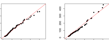
Figure 3: Power law fit for TCR data. QQ plot of the TCR data against quantiles of a power law distribution with $\beta_{1}=0.87$ ($SE=.05$) and $\beta_{2}=0.97$ ($SE=.05$) values fitted via the least squares method.

To compare this finding with a more standard parametric analysis, we additionally fitted, with the least squares method, the counts of $165$ receptor types in two populations to the power law distributions. Since the respective exponent values for the two fitted populations were found to be different, with $\beta_{1}=.87$ (for antibiotic treated mice) and $\beta_{2}=.97$ (for untreated), the parametric analysis confirmed the findings of Algorithm 1. For illustration, the plots of the fitted power law quantiles versus the empirical ones are presented in Figure 3. Additionally, the diversity of each of the TCR populations in terms of its respective Renyi entropy ${\cal H}_{1/2}$ and the Hill number $ENC_{1/2}$ as well as the diversity difference measured by the Renyi divergence ${\cal D}_{1/2}$ are listed in Table 1, along with the corresponding asymptotic confidence intervals obtained via Theorems 1 and 2. As seen from the values in Table 1, although the diversity of each of the NGS populations was relatively similar in terms of the two populations count patterns, it differed in terms of the specific TCR types expressed.

4.2.2 Gene Expression Profiling

Beyond Algorithm 1, the results of Section 3 may be applied to facilitate various other biodiversity analysis, for instance, in simultaneous comparison of several pairs of molecular samples. We illustrate this with an NGS data example from the recent hepatocellular carcinoma (HCC) study in Chan et al (2014) which we obtained through the gene expression omnibus (GEO) database. The GEO dataset consists of HCC tumor-infected ($T$) and healthy liver ($N$) tissue samples from three individuals denoted below as follows in relation to their original database designations $T1=HCC448T,T2=HCC473T,T3=HCC510T$ and $N1=HCC448N,N2=HCC473N,N3=HCC510N$. For this dataset one of the questions of research interest was whether the expression profiles of genes associated with regulation of cell proliferation and programmed cell death differ across $T$ and $N$ samples as well as across individuals (cf., e.g., Kong et al 2013). To address this specific question, in contrast with the previous TCR example, we were thus only interested in a pre-selected subset of the NGS counts. The final values of $m=1332$ and $n$ between 1.2 and 1.9 million reads were obtained after aligning the pre-selected NGS fragments to the HG19 reference genome with the Tophat2/Bowtie2 software (Kim et al, 2013) and performing the transcript annotation with the Ensembl genome browser (www.ensembl.org). After the final fragments-to-counts conversion, our data analysis was performed in three steps. First, the null hypothesis of the tissue homogeneity $H_{0}^{all}=\{T_{1}=N_{1}=T_{2}=N_{2}=T_{3}=N_{3}\}$ was tested (and rejected) based on the result of Theorem 4 and the corresponding asymptotic $p$-value obtained from the $\chi^{2}(3)$ distribution. Next, the hypothesis of the across-individuals homogeneity was tested by evaluating three pairwise null hypothesis $H_{0}^{ij}=\{{\cal D}_{1/2}(T_{i},N_{i})={\cal D}_{1/2}(T_{j},N_{j})]\},$ $1\leq i<j\leq 3$ (each rejected) based on Theorem 4. Finally, having rejected the homogeneity hypothesis we have used the result of Theorem 2 to quantify the differences between the three sets of $T$ and $N$ tissue samples. The details of the analysis are presented in Table 2. As seen from the numerical results, it seems that despite the large individual differences between patients, the set of $m=1332$ genes associated with cell proliferation and death may be used to distinguish between T-type and N-type samples in HCC patients.

Hypothesis	Statistic	$P$-value	${\cal D}_{1/2}$ Value (CI)
$H_{0}^{all}$	$\sum w_{i}[{\cal D}_{1/2}(i)-\mu_{i}]^{2}$	$<0.001$	NA
$H_{0}^{1,2}$	${\cal D}_{1/2}(1)-{\cal D}_{1/2}(2)$	$<0.01$	${\cal D}_{1/2}(1)$=0.553 (0.551, 0.555)
$H_{0}^{2,3}$	${\cal D}_{1/2}(2)-{\cal D}_{1/2}(3)$		${\cal D}_{1/2}(2)$=0.292 (0.291, 0.294)
$H_{0}^{3,1}$	${\cal D}_{1/2}(3)-{\cal D}_{1/2}(1)$		${\cal D}_{1/2}(3)$= 0.346 (0.345 0.348)

Table 2: The $95\%$ confidence intervals for the pairwise symmetric Renyi Divergence ${\cal D}_{1/2}$ between the tumor and control (healthy) tissues from three individuals based on the profile of expression of pre-selected $m=1332$ transcripts related to cell proliferation. Here ${\cal D}_{1/2}(i)$ denotes ${\cal D}_{1/2}(T_{i},N_{i}).$

5 Summary and Conclusions

We derived two sets of limit theorems for the Renyi entropy and divergence statistics. The first set of results holds for lineralizeable statistics (their first order Taylor approximations exist) whereas the second one holds in the degenerate case (when the first order approximations vanish) and requires analyzing the quadratic terms in the Taylor expansions. Our Renyi entropy limit theorems complement those obtained elsewhere for the Shannon entropy and divergence.

Based on the CLT results we have proposed here a new framework for analyzing molecular diversity of molecular (especially NGS) data based on the idea of analyzing the frequency/contingency tables where cell counts are highly unbalanced (for instance, as arriving from mixtures of heavy tailed, power-law type and uniform distributions) and the number of cells or, equivalently, the counts distribution support size $m$, increases with the sample size $n$. For analyzing such tables, we suggested using the empirical Renyi entropy and divergence as the statistical measures of, respectively, diversity and pairwise similarity of different molecular sub-populations.

In the two examples of NGS analysis we have shown how the Renyi entropy methods may be used for filtering out low frequency noise and for establishing valid confidence bounds in pairwise divergence analysis for pre-selected transcripts. However, it was also seen that in order to apply our CLT results the number of transcripts had to be small relative to the sequencing depth. For the special class of heavy-tailed power law distributions, our results in particular indicate that the appropriate entropy CLTs are valid (and thus so is our proposed analysis framework) when, roughly speaking, $m/\sqrt{n}\to 0$ and not otherwise. As such restriction may be often limiting in very high diversity NGS data, other statistics beyond those discussed here and not requiring such condition could be also of interest. We hope to pursuing this matter further in our future work.

Appendix

Appendix A Proofs for Non-Degenerate Projections (Section 3.1)

Auxiliary Results

First, we establish the following simple result on binomial moments.

Lemma 3 (Binomial moment bound).

Let $[x]$ denote the largest integer smaller or equal to $x$ and let $\hat{p}_{n}$ be an empirical binomial proportion from $n$ independent Bernoulli trials with the success probability $0<p_{n}<1$. Assume $np_{n}\to\infty$ as $n\to\infty$. Then for any integer $d\geq 1$ and sufficiently large $n$

$$|E\left(\hat{p}_{n}n-p_{n}n\right)^{d}|\leq C_{d}\,(np_{n})^{[d/2]}$$

for some universal ($n$ free) constant $C_{d}$.

Proof.

Let $X$ be a binomial $Bin(n,p_{n})$ random variable and set $\mu=np_{n}$. Then (see e.g, Knoblauch (2008))

$$E(X-\mu)^{d}=\sum_{i=0}^{d}\binom{d}{i}(-\mu)^{d-i}EX^{i}=\sum_{i=0}^{d}\binom{d}{i}(-\mu)^{d-i}\sum_{k=0}^{i}\genfrac{\{}{\}}{0.0pt}{}{i}{k}p_{n}^{k}n^{\underline{k}},$$

where $\genfrac{\{}{\}}{0.0pt}{}{i}{k}$ denotes a Stirling number of the second kind (i.e. the number of ways to partition a set of $i$ objects into $k$ non-empty subsets) and $n^{\underline{k}}=n(n-1)\cdots(n-k+1)$. Let

$$c_{d,k}=\sum_{i=d-k}^{d}(-1)^{d-i}\binom{d}{i}\genfrac{\{}{\}}{0.0pt}{}{i}{i-d+k}=\sum_{i=0}^{k}(-1)^{i}\binom{d}{i}\genfrac{\{}{\}}{0.0pt}{}{d-i}{k-i}$$

denote the coefficient at $\mu^{k}$ in the expression for $E(X-\mu)^{d}$. Then for $1\leq k\leq d$

$$c_{d+1,k}=d\,c_{d-1,k-1}+k\,c_{d,k}.$$ (A.1)

Indeed,

$$d\,c_{d-1,k-1}+k\,c_{d,k}$$

$$=d\sum_{i=0}^{k-1}(-1)^{i}\binom{d-1}{i}\genfrac{\{}{\}}{0.0pt}{}{d-i-1}{k-i-1}+k\sum_{i=0}^{k}(-1)^{i}\binom{d}{i}\genfrac{\{}{\}}{0.0pt}{}{d-i}{k-i}$$

$$=\sum_{i=0}^{k-1}(-1)^{i}\binom{d}{i+1}(i+1)\genfrac{\{}{\}}{0.0pt}{}{d-i-1}{k-i-1}+k\sum_{i=1}^{k}(-1)^{i}\binom{d}{i}\genfrac{\{}{\}}{0.0pt}{}{d-i}{k-i}+k\,\genfrac{\{}{\}}{0.0pt}{}{d}{k}$$

$$=\sum_{i=1}^{k-1}(-1)^{i}\binom{d}{i}\left((k-i)\genfrac{\{}{\}}{0.0pt}{}{d-i}{k-i}+\genfrac{\{}{\}}{0.0pt}{}{d-i}{k-i-1}\right)+k\,\genfrac{\{}{\}}{0.0pt}{}{d}{k}-\sum_{i=1}^{k-1}(-1)^{i}\binom{d}{i}\genfrac{\{}{\}}{0.0pt}{}{d-i}{k-i-1}$$

and, using the recursions for the Stirling numbers and the binomial coefficients,

$$=\sum_{i=1}^{k-1}(-1)^{i}\left(\binom{d+1}{i}-\binom{d}{i-1}\right)\genfrac{\{}{\}}{0.0pt}{}{d-i+1}{k-i}+\genfrac{\{}{\}}{0.0pt}{}{d+1}{k}-\genfrac{\{}{\}}{0.0pt}{}{d}{k-1}-\sum_{i=1}^{k-1}(-1)^{i}\binom{d}{i}\genfrac{\{}{\}}{0.0pt}{}{d-i}{k-i-1}$$

$$=c_{d+1,k}+0.$$

Let us argue that for any $d\geq 1$ we have

$$c_{d,k}=0\quad\text{for $k$ such that $d/2<k\leq d$}.$$ (A.2)

The proof of (A.2) is by induction with respect to $d\geq 1$. Note that the statement is true for $d=1$ due to $c_{d,d}=0$ for $d\geq 1$ (but $c_{0,0}=1$). Now, if $k>(d+1)/2$ then $k-1>(d-1)/2$ and $k>d/2$ and thus (A.1) implies $c_{d+1,k}=0$ for $k>(d+1)/2$ since the induction assumption implies $c_{d-1,k-1}=c_{d,k}=0$. Hence (A.2) holds and consequently the highest power of $\mu$ in the expansion of $E(X-\mu)^{d}$ cannot exceed $d/2$. This yields the assertion of the lemma.

∎

Lemma 4.

Set $\tilde{W}_{n}^{(\alpha)}=(W_{n}^{(\alpha)}-EW_{n}^{(\alpha)})/(VarW_{n}^{(\alpha)})^{1/2}$. Under the assumptions of Theorem 1, the Lindeberg condition

$$\forall_{\varepsilon>0}\ E(\tilde{W}_{n}^{(\alpha)})^{2}I(|\tilde{W}_{n}^{(\alpha)}|>\varepsilon\sqrt{n})\to 0,\quad n\to\infty$$ (A.3)

is satisfied. Consequently,

$$\sqrt{n}\sum_{i=1}^{n}\tilde{W}_{ni}^{(\alpha)}\Rightarrow N(0,1)$$

with $n$ iid random variables $\tilde{W}_{ni}^{(\alpha)}$ equidistributed with $\tilde{W}_{n}^{(\alpha)}$. Moreover, the result remains true if we replace above $W_{n}^{(\alpha)}$ by $V_{n}^{(\alpha)}$ under the assumptions of Theorem 2.

Proof.

We shall only prove the statement for $W_{n}^{(\alpha)}$, as the proof for $V_{n}^{(\alpha)}$ is similar. For notational convenience, set $\sigma^{2}_{n}=VarW_{n}^{(\alpha)}$, $\mu_{n}=EW_{n}^{(\alpha)}$ and $\tilde{W}_{n}=\tilde{W}_{n}^{(\alpha)}$. In view of (3.1) we have as $n\to\infty$

$$\frac{\mu_{n}}{\sqrt{n}\sigma_{n}}=\frac{\alpha\sum p_{i}^{\alpha}}{\sqrt{n}\sigma_{n}}\leq\frac{\sum p_{i}^{\alpha-1}}{\sqrt{n}\sigma_{n}}\to 0.$$ (A.4)

Note that $\tilde{W}_{n}=\alpha\sigma_{n}^{-1}\sum p_{i}^{\alpha-1}(\delta_{i}-p_{i})$ where the vector $(\delta_{1},\ldots,\delta_{m})$ represents a single trial multinomial random vector with parameters $(p_{1},\ldots,p_{m})$. For any $\varepsilon>0$

$$E\tilde{W}_{n}^{2}I(|\tilde{W}_{n}|>\varepsilon\sqrt{n}) =\alpha^{2}\sigma_{n}^{-2}E(\sum p_{i}^{\alpha-1}(\delta_{i}-p_{i}))^{2}I(|\tilde{W}_{n}|>\varepsilon\sqrt{n})$$

$$\leq\alpha^{2}\sigma_{n}^{-2}E[(\sum p_{i}^{\alpha})^{2}+\sum\delta_{i}p_{i}^{2(\alpha-1)}]I(|\tilde{W}_{n}|>\varepsilon\sqrt{n}).$$ (A.5)

Since by (A.4) $\mu_{n}=o((n\sigma^{2}_{n})^{1/2})$, then by the definition of $\delta_{i}$, for sufficiently large $n$ we have

$$\{\omega:|\tilde{W}_{n}|>\varepsilon\sqrt{n}\} =\{\omega:\alpha|\sigma_{n}^{-1}\sum p_{i}^{\alpha-1}(\delta_{i}-p_{i})|>\varepsilon\sqrt{n}\}$$

$$=\{\omega:\delta_{i}=1\text{ for $i$ such that }\alpha|p_{i}^{\alpha-1}-\mu_{n}|>\varepsilon\sqrt{n}\sigma_{n}\}$$

$$\subset\{\omega:\delta_{i}=1\text{ for $i$ such, that }\alpha p_{i}^{\alpha-1}>\frac{\varepsilon}{2}\sqrt{n}\sigma_{n}\}\}$$

$$=:\{\omega:\delta_{i}=1\text{ for }i\in J_{n}\}$$

where the last equality defines the set of indices $J_{n}$. Note that the size of the set $J_{n}$ satisfies $|J_{n}|\to 0$ as $n\to\infty$, due to  $\max_{1\leq i\leq m_{n}}p_{i}^{\alpha-1}/\sqrt{n}\sigma_{n}\to 0$ as $n\to\infty$, which is implied by (3.1). This and (A) give therefore (at least for large $n$)

$$E\tilde{W}_{n}^{2}I(|\tilde{W}_{n}|>\varepsilon\sqrt{n}) \leq\sigma_{n}^{-2}\sum_{i\in J_{n}}p_{i}(\mu_{n}^{2}+\alpha^{2}p_{i}^{2(\alpha-1)})=(\mu_{n}/\sigma_{n})^{2}\sum_{i\in J_{n}}p_{i}+\alpha^{2}\sigma_{n}^{-2}\sum_{i\in J_{n}}p_{i}^{2\alpha-1}$$

$$\leq 2\alpha(\mu_{n}/\sigma_{n})^{2}\sum p_{i}^{\alpha}/(\varepsilon\sqrt{n}\sigma_{n})+(\mu_{n}^{2}/\sigma_{n}^{2}+1)\sum_{i\in J_{n}}p_{i}^{2\alpha-1}/(\mu_{n}^{2}+\sigma_{n}^{2})\to 0$$

as $n\to\infty$, since $\sup_{n}(\mu_{n}/\sigma_{n})^{2}<\infty$ by the assumptions of Theorem 1 and $\alpha^{2}\sum p_{i}^{2\alpha-1}=\mu_{n}^{2}+\sigma_{n}^{2}$. The weak convergence assertion follows now by the Lindeberg central limit theorem (see, e.g, Shao (2003) Chapter 1).

∎

Proof of Theorem 1

Let us first establish part $(ii)$. Note that (3.1) implies that

$$a_{n}^{2}=n/VarW_{n}^{(\alpha)}\to\infty,$$ (A.6)

in view of

$$a_{n}^{2}\sum p_{i}^{\alpha-1}/n\geq\alpha^{2}a_{n}^{2}\sum p_{i}^{2\alpha-1}/n\geq 1$$

which yields $a_{n}\geq(nVarW_{n}^{(\alpha)})^{1/2}(\sum p_{i}^{\alpha-1})^{-1}.$ By Taylor’s expansion

$${\cal S}_{\alpha}(\hat{\bm{p}})-{\cal S}_{\alpha}({\bm{p}})=\sum\hat{p}_{i}^{\alpha}-\sum p_{i}^{\alpha}=\sum\alpha p_{i}^{\alpha-1}(\hat{p}_{i}-p_{i})+R_{n}$$ (A.7)

where

$$R_{n}=\sum\binom{\alpha}{2}p_{i}^{\alpha}\left(\frac{\hat{p}_{i}-p_{i}}{p_{i}}\right)^{2}\left(\theta_{i}\left(\frac{\hat{p}_{i}}{p_{i}}-1\right)+1\right)^{\alpha-2}\quad\text{for some random }\theta_{i}\in(0,1).$$

Fixing $\delta\in(0,1/2)$, for any $\varepsilon>0$, we have

$$P(|R_{n}|>\varepsilon) =P\left(|R_{n}|>\varepsilon,\max_{i}\left|\theta_{i}\left(\frac{\hat{p}_{i}}{p_{i}}-1\right)\right|\leq\delta\right)+P\left(|R_{n}|>\varepsilon,\max_{i}\left|\theta_{i}\left(\frac{\hat{p}_{i}}{p_{i}}-1\right)\right|>\delta\right)$$

$$\leq P\left(|R_{n}|>\varepsilon,\max_{i}\left|\theta_{i}\left(\frac{\hat{p}_{i}}{p_{i}}-1\right)\right|\leq\delta\right)+P\left(\max_{i}\left|\theta_{i}\left(\frac{\hat{p}_{i}}{p_{i}}-1\right)\right|>\delta\right)$$

$$=:(I)+(II).$$

First, note

$$(I)\leq\frac{1}{\varepsilon}E|R_{n}|I\!\left(\max_{i}\left|\theta_{i}\left(\frac{\hat{p}_{i}}{p_{i}}-1\right)\right|\leq\delta\right)\leq\frac{1}{\varepsilon}\binom{\alpha}{2}\sum p_{i}^{\alpha}E\left(\frac{\hat{p}_{i}-p_{i}}{p_{i}}\right)^{2}\left(1-\delta\right)^{\alpha-2}\leq\frac{C_{1}}{\varepsilon\,n}\sum p_{i}^{\alpha-1}.$$

Now, recall the condition (2.5) and consider $d\geq 1$ large enough so that $d\tau>1$ and hence $(np_{\ast})^{-d}\leq n^{-1}$ for sufficiently large $n$. Applying Bool’s (subadditivity) inequality bound and Lemma 3 to the $2d$-th central moments of the $\hat{p}_{i}$’s, we get

$$(II)\leq P\left(\max_{i}\left|p_{i}^{(\alpha-1)/2d}\left(\frac{\hat{p}_{i}}{p_{i}}-1\right)\right|>\delta\right)\leq\sum\frac{C_{2}\,p_{i}^{\alpha-1}}{\delta^{2d}\,n^{d}p_{i}^{d}}\leq\frac{C_{3}}{\delta^{2d}\,n}\sum p_{i}^{\alpha-1}$$

where $C_{1},C_{2},C_{3}$ are constants independent of $n$ and $p_{i}$ (with $C_{2}$ being $C_{2d}$ of Lemma 3). Therefore, for any $\varepsilon>0$ and the numerical sequence $a_{n}=|a_{n}|=(n/VarW_{n}^{(\alpha)})^{1/2}\to\infty$ (cf. (A.6)) as well as a possibly different set of constants $C_{1},C_{2},C_{3}$

$$P(|a_{n}R_{n}|>\varepsilon)\leq\max\left(\frac{C_{1}a_{n}}{\varepsilon},\frac{C_{2}}{\delta^{2d}}\right)\sum p_{i}^{\alpha-1}/n\leq C_{3}a_{n}\sum p_{i}^{\alpha-1}/n\to 0$$ (A.8)

as $n\to\infty$, due to (3.1). Note that the random variable $\alpha\sum p_{i}^{\alpha-1}(\hat{p}_{i}-p_{i})$ has the same distribution as ${\cal W}_{n}=\sum(W_{ni}^{(\alpha)}-EW_{ni}^{(\alpha)})/n$, with iid random variables $W_{ni}^{(\alpha)}$distributed as (2.6) and that, due to (A.8), $a_{n}R_{n}=R_{n}/(Var{\cal W}_{n})^{1/2}=o_{p}(1)$. Since Lemma 4 ensures that $({\cal W}_{n}-E{\cal W}_{n})/(Var{\cal W}_{n})^{1/2}\Rightarrow N(0,1)$, the result follows.

To argue part $(i)$, note that from the definition of (2.6) we have $EW_{n}^{(\alpha)}=\alpha^{2}{\cal S}_{\alpha}({\bm{p}})=\alpha^{2}\sum p_{i}^{\alpha}\geq\alpha^{2}$ and by (A.6) $\tilde{a}_{n}=(n{\cal S}_{\alpha}({\bm{p}})^{2}/VarW_{n}^{(\alpha)})^{1/2}\to\infty$. Consequently, part $(i)$ follows immediately from part $(ii)$.

Finally, we show part $(iii)$. Consider arbitrary $\delta\in(0,1)$ and note that on the events $|{\cal S}_{\alpha}(\hat{\bm{p}})/{\cal S}_{\alpha}({\bm{p}})-1|\leq\delta$, by Taylor’s expansion for $|x|<1$, we have

$$\log(1+x)=x-\frac{x^{2}}{2(1+\theta x)^{2}},$$ (A.9)

where $\theta\in(0,1)$ and hence

$$(1-\alpha)(\mathcal{H}_{\alpha}(\hat{\bm{p}})-\mathcal{H}_{\alpha}({\bm{p}}))=\log\left(\frac{{\cal S}_{\alpha}(\hat{\bm{p}})}{{\cal S}_{\alpha}({\bm{p}})}\right) =\frac{{\cal S}_{\alpha}(\hat{\bm{p}})}{{\cal S}_{\alpha}({\bm{p}})}-1-\frac{\left(\frac{{\cal S}_{\alpha}(\hat{\bm{p}})}{{\cal S}_{\alpha}({\bm{p}})}-1\right)^{2}}{2(1+\theta(\frac{{\cal S}_{\alpha}(\hat{\bm{p}})}{{\cal S}_{\alpha}({\bm{p}})}-1))^{2}}$$

$$=\frac{{\cal S}_{\alpha}(\hat{\bm{p}})-{\cal S}_{\alpha}({\bm{p}})}{{\cal S}_{\alpha}({\bm{p}})}+T_{n}.$$ (A.10)

where the last equation defines $T_{n}$. By applying again the expansion argument used in the proof of part $(ii)$ with ${\cal S}_{\alpha}(\hat{\bm{p}})/{\cal S}_{\alpha}({\bm{p}})$ in place of ${\cal S}_{\alpha}(\hat{\bm{p}}$) and $R_{n}/{\cal S}_{\alpha}({\bm{p}})$ in place of $R_{n}$ and the sequence $\tilde{a}_{n}=(n{\cal S}_{\alpha}({\bm{p}})^{2}/VarW_{n}^{(\alpha)})^{1/2}\to\infty$, we see that

$$\tilde{a}_{n}({\cal S}_{\alpha}(\hat{\bm{p}})/{\cal S}_{\alpha}({\bm{p}})-1)=\sqrt{n}\,\frac{{\cal S}_{\alpha}(\hat{\bm{p}})-{\cal S}_{\alpha}({\bm{p}})}{(VarW_{n}^{(\alpha)})^{1/2}}\Rightarrow N(0,1)$$ (A.11)

as $n\to\infty.$ Note that for any $\varepsilon>0$

$$P(\tilde{a}_{n}|T_{n}|>\varepsilon,|{\cal S}_{\alpha}(\hat{\bm{p}})/{\cal S}_{\alpha}({\bm{p}})-1|\leq\delta)\leq P\left(\tilde{a}_{n}\frac{|{\cal S}_{\alpha}(\hat{\bm{p}})/{\cal S}_{\alpha}({\bm{p}})-1|}{2(1-\delta)^{2}}>\varepsilon/\delta\right)$$

and therefore

$$P(\tilde{a}_{n}|T_{n}|>\varepsilon)\leq P(|{\cal S}_{\alpha}(\hat{\bm{p}})/{\cal S}_{\alpha}({\bm{p}})-1|>\delta)+P\left(\tilde{a}_{n}|{\cal S}_{\alpha}(\hat{\bm{p}})/{\cal S}_{\alpha}({\bm{p}})-1|>2\varepsilon(1-\delta)^{2}/\delta\right).$$ (A.12)

In view of $(i)$ and (A.11), denoting the absolute value of $N(0,1)$ by $|N|$, (A.12) yields

$$\limsup_{n}P(\tilde{a}_{n}|T_{n}|>\varepsilon)\leq 0+P(|N|\geq 2\varepsilon(1-\delta)^{2}/\delta).$$

By taking $\delta>0$ to be sufficiently small we get

$$\limsup_{n}P(\tilde{a}_{n}|T_{n}|>\varepsilon)\leq\gamma$$

for arbitrary $\gamma>0$, and therefore $\limsup_{n}P(\tilde{a}_{n}|T_{n}|>\varepsilon)=0$. Thus for any $x$, we have

$$P\left(\sqrt{n}\,\frac{(1-\alpha)(\mathcal{H}_{\alpha}(\hat{\bm{p}})-\mathcal{H}_{\alpha}({\bm{p}}))}{\alpha\,{\cal CV}(W_{n}^{(\alpha)})}\leq x\right)=P\left(\sqrt{n}\,\frac{{\cal S}_{\alpha}(\hat{\bm{p}})-{\cal S}_{\alpha}({\bm{p}})}{(VarW_{n}^{(\alpha)})^{1/2}}\leq x\right)+o_{p}(1)$$

and the result follows from part $(ii)$. ∎

Proof of Theorem 2

The proof follows closely that of Theorem 1 with some obvious modifications. For illustration, we shall only argue part $(ii)$. Let us first note that, in parallel with (A.6), $b_{n}=(n/VarV_{n}^{(\alpha)})^{1/2}\to\infty.$ Indeed, since

$$b_{n}^{2}\geq\frac{n}{E(V_{n}^{(\alpha)})^{2}}\geq\frac{n}{2\sum_{ij}p_{ij}\left[\left(\frac{q_{i}}{p_{i}}\right)^{2(1-\alpha)}+\left(\frac{p_{j}}{q_{j}}\right)^{2\alpha}\right]}\geq\frac{n}{2\sum\left(\frac{q_{i}}{p_{i}}\right)^{1-\alpha}+2\sum\left(\frac{p_{i}}{q_{i}}\right)^{\alpha}},$$

therefore

$$2b_{n}\geq\frac{(nVarV_{n}^{(\alpha)})^{1/2}}{\sum\left(\frac{q_{i}}{p_{i}}\right)^{1-\alpha}+\sum\left(\frac{p_{i}}{q_{i}}\right)^{\alpha}}\to\infty$$ (A.13)

due to (3.3). Next, we show that the limiting distribution is determined by the projection $V_{n}^{(\alpha)}$. By the bivariate Taylor expansion, one obtains

$$b_{n}({\cal S}_{\alpha}(\hat{\bm{p}},\hat{{\bm{q}}})-{\cal S}_{\alpha}({\bm{p}},{\bm{q}}))=b_{n}\left(\alpha\sum_{i}(q_{i}/p_{i})^{1-\alpha}(\hat{p}_{i}-p_{i})+(1-\alpha)\sum_{i}(p_{i}/q_{i})^{\alpha}(\hat{q}_{i}-q_{i})\right)+b_{n}R_{n}$$

where

$$R_{n}=\left.\sum_{i}\sum_{\{(k,l):k,l\geq 0,k+l=2\}}\frac{\partial^{2}\tilde{p}_{i}^{\alpha}\tilde{q}_{i}^{1-\alpha}}{\partial^{k}\tilde{p}_{i}\partial^{l}\tilde{q}_{i}}\right|_{(\tilde{p}_{i},\tilde{q}_{i})=(p_{i},q_{i})+\theta_{i}(\hat{p}_{i}-p_{i},\hat{q}_{i}-q_{i})}\frac{(\hat{p}_{i}-p_{i})^{k}(\hat{q}_{i}-q_{i})^{l}}{k!\,l!}$$

and $|\theta_{i}|\leq 1$ for all $i$. Since for the mixed derivatives term, by virtue of the elementary inequality $2ab\leq a^{2}+b^{2}$ (with $a=\alpha(\hat{p}_{i}-p_{i})/\tilde{p}_{i}$ and $b=(1-\alpha)(\hat{q}_{i}-q_{i})/\tilde{q}_{i}$) we have

$$2\alpha(1-\alpha)\sum\tilde{p}_{i}^{\alpha-1}\tilde{q}_{i}^{-\alpha}(\hat{p}_{i}-p_{i})(\hat{q}_{i}-q_{i})\leq\alpha^{2}\sum\tilde{p}_{i}^{\alpha-2}\tilde{q}_{i}^{1-\alpha}(\hat{p}_{i}-p_{i})^{2}+(1-\alpha)^{2}\sum\tilde{p}_{i}^{\alpha}\tilde{q}_{i}^{-\alpha-1}(\hat{q}_{i}-q_{i})^{2},$$

therefore

$$b_{n}R_{n}\leq 2b_{n}(R_{n}^{(1)}+R_{n}^{(2)})$$

with

$$R_{n}^{(1)}=\sum_{i}p_{i}^{\alpha}q_{i}^{1-\alpha}\left(\theta_{i}\left(\frac{\hat{p}_{i}}{p_{i}}-1\right)+1\right)^{\alpha-2}\left(\theta_{i}\left(\frac{\hat{q}_{i}}{q_{i}}-1\right)+1\right)^{1-\alpha}\left(\frac{\hat{p}_{i}-p_{i}}{p_{i}}\right)^{2}$$

and

$$R_{n}^{(2)}=\sum_{i}p_{i}^{\alpha}q_{i}^{1-\alpha}\left(\theta_{i}\left(\frac{\hat{p}_{i}}{p_{i}}-1\right)+1\right)^{\alpha}\left(\theta_{i}\left(\frac{\hat{q}_{i}}{q_{i}}-1\right)+1\right)^{-\alpha-1}\left(\frac{\hat{q}_{i}-q_{i}}{q_{i}}\right)^{2}.$$

Clearly, it suffices now to show only that $b_{n}R_{n}^{(i)}=o_{p}(1)$ for $i=1,2$. We only prove the second relation, the other one follows similarly. Analogously as in the proof of Theorem 1 taking some small $\delta>0$ we have

$$P(b_{n}R_{n}^{(2)}>\varepsilon) \leq P\left(b_{n}R_{n}^{(2)}>\varepsilon,\max_{i}\left\{\left|\theta_{i}\left(\frac{\hat{p}_{i}}{p_{i}}-1\right)\right|+\left|\theta_{i}\left(\frac{\hat{q}_{i}}{q_{i}}-1\right)\right|\right\}\leq\delta\right)$$

$$+P\left(\max_{i}\left\{\left|\theta_{i}\left(\frac{\hat{p}_{i}}{p_{i}}-1\right)\right|+\left|\theta_{i}\left(\frac{\hat{q}_{i}}{q_{i}}-1\right)\right|\right\}>\delta\right)$$

$$=:(I)+(II).$$

Apropos $(I)$, for some universal ($n$-free and $\delta$-free) constant $C$ we have

$$(I)\leq b_{n}\varepsilon^{-1}\sum_{i}p_{i}^{\alpha}q_{i}^{1-\alpha}\left(1+\delta\right)^{\alpha}\left(1-\delta\right)^{-\alpha-1}E\left(\frac{\hat{q}_{i}-q_{i}}{q_{i}}\right)^{2}\leq C\varepsilon^{-1}\sum p_{i}^{\alpha}q_{i}^{-\alpha}/(nVarV_{n}^{(\alpha)})^{1/2}\to 0$$

by (3.3). Apropos $(II)$, we have

$$(II)\leq P\left(\max_{i}\left|\left(\frac{\hat{p}_{i}}{p_{i}}-1\right)\right|>\delta/2\right)+P\left(\max_{i}\left|\left(\frac{\hat{q}_{i}}{q_{i}}-1\right)\right|>\delta/2\right)=:(IIa)+(IIb)$$

Note that for $d$ large enough so that $d\tau>1$, in view of (2.5) and the Boole inequality bound combined with the result of Lemma 3,

$$(IIa) \leq P\left(\max_{i}\left|\max\left\{\left(\frac{p_{i}}{q_{i}}\right)^{\frac{\alpha}{2d}},\left(\frac{q_{i}}{p_{i}}\right)^{\frac{1-\alpha}{2d}}\right\}\left(\frac{\hat{p}_{i}}{p_{i}}-1\right)\right|>\delta/2\right)\leq\left(\frac{2}{\delta}\right)^{2d}\sum\max\left\{\left(\frac{p_{i}}{q_{i}}\right)^{\alpha},\left(\frac{q_{i}}{p_{i}}\right)^{1-\alpha}\right\}(np_{i})^{-d}$$

$$\leq\left(\frac{2}{\delta}\right)^{2d}n^{-1}\sum\left[\left(\frac{p_{i}}{q_{i}}\right)^{\alpha}+\left(\frac{q_{i}}{p_{i}}\right)^{1-\alpha}\right]\leq\left(\frac{2}{\delta}\right)^{2d}b_{n}n^{-1}\sum\left[\left(\frac{p_{i}}{q_{i}}\right)^{\alpha}+\left(\frac{q_{i}}{p_{i}}\right)^{1-\alpha}\right]\rightarrow 0$$

by (A.13) and (3.3). Similarly,

$$(IIb) \leq P\left(\max_{i}\left|\max\left\{\left(\frac{p_{i}}{q_{i}}\right)^{\frac{\alpha}{2d}},\left(\frac{q_{i}}{p_{i}}\right)^{\frac{1-\alpha}{2d}}\right\}\left(\frac{\hat{q}_{i}}{q_{i}}-1\right)\right|>\delta/2\right)\leq\left(\frac{2}{\delta}\right)^{2d}b_{n}n^{-1}\sum\left[\left(\frac{p_{i}}{q_{i}}\right)^{\alpha}+\left(\frac{q_{i}}{p_{i}}\right)^{1-\alpha}\right]\rightarrow 0$$

and therefore $b_{n}R_{n}^{(2)}=o_{p}(1)$ and by a similar argument $b_{n}R_{n}^{(1)}=o_{p}(1)$. Consequently, $b_{n}R_{n}=o_{p}(1).$ Finally, since the distribution of $\alpha\sum_{i}(q_{i}/p_{i})^{1-\alpha}(\hat{p}_{i}-p_{i})+(1-\alpha)\sum_{i}(p_{i}/q_{i})^{\alpha}(\hat{q}_{i}-q_{i})$ is equal to that of $\sum_{k=1}^{n}(V_{k}^{(n)}-EV_{k}^{(n)})/n$ where $V_{k}^{(n)}$ are independent and distributed according to $V_{n}^{(\alpha)}$ given in (2.7), the result follows by Lemma 4.

Appendix B Proofs for Degenerate Projections (Section 3.2)

Auxiliary Results

The following lemma is cited after Koroljuk and Borovskich (1994, Theorem  4.7.3, page 162).

Lemma 5 (Degenerate $U$-statistic CLT).

Let $X_{1}\ldots,X_{n}$ be a sequence of iid random elements and let

$$U_{n}(X_{1},\ldots,X_{n})=\binom{n}{2}^{-1}\sum_{1\leq k<l\leq n}h_{n}(X_{k},X_{l})$$

be a $U$-statistic of order two with a symmetric, real-valued kernel $h_{n}(x,y)$ which depends on $n$ and satisfies $Eh_{n}(X,y)=0$. Denote also $\Psi_{n}(y,z)=E(h_{n}(X,y)h_{n}(X,z)).$ Assume that $Eh_{n}^{4}<\infty$ and set $\sigma_{n}^{2}=Eh_{n}^{2}$. If the conditions

$$n^{-1}\sigma_{n}^{-4}Eh_{n}^{4}\to 0$$ (B.1)

$$\sigma_{n}^{-4}E\Psi_{n}^{2}\to 0$$ (B.2)

are satisfied, then

$$nU_{n}/(\sqrt{2}\sigma_{n})\Rightarrow N(0,1).$$

∎

Proof of Lemma 2

We start by showing $(i)$. To this end, let $X_{k}$ for $k=1,\ldots,n$ be iid single trial multinomial variables with parameter ${\bm{p}}$ and denote $I(X_{k}=i)=\delta_{i}(X_{k})$. Note the identity

$${\cal X}^{2}_{\bm{p}}(\hat{\bm{p}},{\bm{p}})-m+1 =n\sum p_{i}^{-1}(n^{-1}\sum_{k}\delta_{i}(X_{k})-p_{i})^{2}-m+1$$

$$=n^{-1}\sum p_{i}^{-1}\sum_{k\neq l}\delta_{i}(X_{k})\delta_{i}(X_{l})+n^{-1}\sum p_{i}^{-1}\sum_{k}\delta_{i}(X_{k})-n-m+1$$

$$=n^{-1}\sum_{k\neq l}(\sum p_{i}^{-1}\delta_{i}(X_{k})\delta_{i}(X_{l})-1)+n^{-1}\sum_{k}(\sum p_{i}^{-1}\delta_{i}(X_{k})-m)$$

$$=(n-1)U_{n}^{(1)}+R_{n}^{(1)}.$$

Here $U_{n}^{(1)}$ is the $U$-statistic with order-two kernel $h_{n}(X_{1},X_{2})=\sum_{i}p_{i}^{-1}I(X_{1}=X_{2}=i)-1$ which is degenerate, i.e., satisfies $Eh_{n}(X_{1},x_{2})=0$. The remaining term $R_{n}^{(1)}=n^{-1}\sum_{k}(V_{k}-EV_{k})$, where $V_{k}$ are iid, equidistributed with, say, $V$ such that $P(V=p_{i}^{-1})=p_{i}$. We will argue that

$$(n-1)U_{n}^{(1)}/\sqrt{2(m-1)}\Rightarrow N(0,1)$$ (B.3)

and $R_{n}^{(1)}/\sqrt{m}=o_{p}(1).$ The second relation follows easily, since $m^{-1}VarR_{n}^{(1)}=(nm)^{-1}VarV=(nm)^{-1}(\sum p_{i}^{-1}-m^{2})\to 0$ by assumption (3.5).

The convergence (B.3) will follow from Lemma 5 and Slutsky’s theorem upon checking the conditions (B.1) and (B.2). To this end note that in the notation of Lemma 5 $\sigma_{n}^{2}=Var\,h_{n}=m-1$ since $Var[h_{n}(X_{1},X_{2})]=E[h_{n}(X_{1},X_{2})]^{2}=\sum p_{i}E(p_{i}^{-1}I(X_{1}=i)-1)^{2}=\sum p_{i}E(p_{i}^{-2}I(X_{1}=i)+1-2p_{i}^{-1}I(X_{1}=i))=m-1$. Similarly, $Eh_{n}^{4}=\sum p_{i}E(p_{i}^{-1}I(X_{1}=i)-1)^{4}=\sum(p_{i}^{-2}-4p_{i}^{-1})+6m-3.$ Therefore

$$n^{-1}Eh_{n}^{4}/\sigma_{n}^{4}\leq\frac{\sum(p_{i}^{-2}-4p_{i}^{-1})+6m-3}{n(m-1)^{2}}\leq Cn^{-1}\sum p_{i}^{-2}m^{-2}\to 0$$

due to (3.5) and thus (B.1) follows. In order to verify (B.2), consider first $\Psi_{n}(x,y)=E[h_{n}(X_{1},x)h_{n}(X_{1},y)]=p_{x}^{-1}I(x=y)-1.$ Since $E\Psi_{n}^{2}(X_{1},X_{2})=\sum p_{i}E\Psi_{n}^{2}(X_{1},i)=\sum p_{i}E[p_{i}^{-1}I(X_{1}=i)-1]^{2}=m-1$, then we have $E\Psi_{n}^{2}(X_{1},X_{2})/\sigma_{n}^{4}\to~{}0$ and (B.2) follows as well. Hence (B.3) follows and yields the assertion $(i)$.

Now consider part $(ii)$. In parallel to part $(i)$, define (cf. Section 2) $Z_{k}=(X_{k},Y_{k})$ for $k=1,\ldots,n$ as a sequence of independent bivariate random variables distributed according to $Z=(X,Y)$. Additionally, for $i=1,\ldots,m$, as before let $\delta_{i}(X_{k})=I(X_{k}=i)$, as well as $\delta_{i}(Y_{k})=I(Y_{k}=i)$. Set also $\Delta_{i}(Z_{k})=\Delta_{i}(X_{k},Y_{k})=\delta_{i}(X_{k})-\delta_{i}(Y_{k})$. Note that for given $i$ the $\Delta_{i}(Z_{k})$’s for $k=1,\ldots,n$ are independent variables distributed according to

$$\Delta_{i}(Z)=\begin{cases}0&\text{with prob.}\ 1-2(p_{i}-p_{ii}),\\ 1&\text{with prob.}\ p_{i}-p_{ii}\\ -1&\text{with prob.}\ p_{i}-p_{ii}.\\ \end{cases}$$

In particular, $E\Delta_{i}(Z)=0$ and $E\Delta^{2}_{i}(Z)=2(p_{i}-p_{ii})$. Recall that $\mu_{n}=\sum(1-p_{ii}/p_{i})$ and consider

$${\cal X}^{2}_{2{\bm{p}}}(\hat{\bm{p}},\hat{{\bm{q}}})-\mu_{n}=n^{-1}\sum(2p_{i})^{-1}(\sum_{k}\Delta_{i}(Z_{k}))^{2}-\mu_{n}$$

$$=n^{-1}\sum_{k\neq l}\sum(2p_{i})^{-1}\Delta_{i}(Z_{k})\Delta_{i}(Z_{l})+n^{-1}\sum_{k}\sum(2p_{i})^{-1}(\Delta_{i}^{2}(Z_{k})-2(p_{i}-p_{ii}))$$

$$=(n-1)U_{n}^{(2)}+R_{n}^{(2)}.$$

which parallels the representation in part $(i)$. Regarding $R_{n}^{(2)}$ note that it is, as before, the zero mean sum of independent variables with variance

$$Var\,R_{n}^{(2)} =Var[n^{-1}\sum_{k}\sum_{i}(2p_{i})^{-1}\Delta_{i}^{2}(Z_{k})]=n^{-1}Var[\sum_{i}(2p_{i})^{-1}(\delta_{i}(X)-\delta_{i}(Y))^{2}]$$

$$\leq n^{-1}\sum_{i\neq j}\left((2p_{i})^{-1}+(2p_{j})^{-1}\right)^{2}p_{ij}\leq 2n^{-1}\sum_{i\neq j}\left((2p_{i})^{-2}+(2p_{j})^{-2}\right)p_{ij}$$

$$\leq n^{-1}\sum p_{i}^{-1},$$

where the first inequality above is obtained by applying the second moment bound and noticing that the inner sum consists of either two or zero summands, according to $X\neq Y$ or $X=Y$. The condition (3.5) implies that

$$R_{n}^{(2)}/\sqrt{m}=o_{p}(1).$$ (B.4)

Regarding $U_{n}^{(2)}$, note that it is a $U$-statistic in bivariate variables $Z_{k}$ with second order degenerate kernel given by $h_{n}(Z_{1},Z_{2})=\sum(2p_{i})^{-1}\Delta_{i}(Z_{1})\Delta_{i}(Z_{2})$. Hence, in the notation of Lemma 5, $\sigma_{n}^{2}=Eh_{n}^{2}(Z_{1},Z_{2})=E\left[\sum(2p_{i})^{-1}\Delta_{i}(Z_{1})\Delta_{i}(Z_{2})\right]^{2}=\sum(2p_{i})^{-2}(E\Delta_{i}^{2}(Z_{1}))^{2}+\sum_{i\neq j}(2p_{i})^{-1}(2p_{j})^{-1}(E[\Delta_{i}(Z_{1})\Delta_{j}(Z_{1})])^{2}.$ Since we have $E\Delta_{i}^{2}(Z_{1})=2(p_{i}-p_{ii})$ and $E[\Delta_{i}(Z_{1})\Delta_{j}(Z_{1})]=-E[I(X_{1}=i,Y_{1}=j)+I(X_{1}=j,Y_{1}=i)]=-(p_{ij}+p_{ji})$, it follows that $\sigma_{n}^{2}=\gamma_{n}^{2}$ given in (3.7). Recall (Remark 3.6) that under our assumptions $\sigma_{n}/\sqrt{m}\to 1$ and thus (B.4) implies $R_{n}^{(1)}/\sigma_{n}=o_{p}(1)$.

Now, in order to complete the proof as in part $(i)$, we only need to show that the conditions (B.1) and (B.2) are satisfied for $U_{n}^{(2)}$, since then by Lemma 5 the statement similar to (B.3) holds for part $(ii)$, namely

$$(n-1)U_{n}^{(2)}/(\sqrt{2}\sigma_{n})\Rightarrow N(0,1).$$ (B.5)

To this end note first that by the definition of $\Delta$ variables $\Delta_{i}(Z)=\Delta_{i}^{2p+1}(Z)$ and $\Delta_{i}^{2}(Z)=\Delta_{i}^{2p}(Z)$ for any integer $p\geq 1$. Additionally, since $Z$ is bivariate, for any distinct indices $(i,j,k,l)$ we have $E[\Delta_{i}(Z)\Delta_{j}(Z)\Delta^{2}_{k}(Z)]=E[\Delta_{i}(Z)\Delta_{j}(Z)\Delta_{k}(Z)\Delta_{l}(Z)]=0$. Consequently,

$$Eh_{n}^{4} =E[\sum(2p_{i})^{-1}\Delta_{i}(Z_{1})\Delta_{i}(Z_{2})]^{4}=2^{-4}\{\sum p_{i}^{-4}E[\Delta_{i}^{4}(Z_{1})\Delta_{i}^{4}(Z_{2})]$$

$$\qquad+6\sum_{i\neq j}p_{i}^{-2}p_{j}^{-2}E[\Delta_{i}^{2}(Z_{1})\Delta_{i}^{2}(Z_{2})\Delta_{j}^{2}(Z_{1})\Delta_{j}^{2}(Z_{2})]$$

$$\qquad+4\sum_{i\neq j}p_{i}^{-3}p_{j}^{-1}E[\Delta_{i}^{3}(Z_{1})\Delta_{i}^{3}(Z_{2})\Delta_{j}(Z_{1})\Delta_{j}(Z_{2})]+0\}$$

$$=2^{-4}\{\sum p_{i}^{-4}4(p_{i}-p_{ii})^{2}+6\sum_{i\neq j}p_{i}^{-2}p_{j}^{-2}(p_{ij}+p_{ji})^{2}+4\sum_{i\neq j}p_{i}^{-3}p_{j}^{-1}(p_{ij}+p_{ji})^{2}\}$$

$$=2^{-4}\{\sum p_{i}^{-4}4(p_{i}-p_{ii})^{2}+\sum_{i\neq j}(6p_{i}^{-2}p_{j}^{-2}+4p_{i}^{-3}p_{j}^{-1})(p_{ij}+p_{ji})^{2}\}.$$

In view of the condition (3.6) and Remark 3.6 as well (3.5)

$$\frac{Eh_{n}^{4}}{n\sigma_{n}^{4}}\leq\frac{3}{2\,n(m-2B)^{2}}\sum(p_{i}^{-2}+mB^{2}+B^{2}p_{i}^{-1})\leq\frac{C}{nm^{2}}\sum p_{i}^{-2}\to 0$$

for some universal $C>0$ and hence (B.1) holds. In order to argue (B.2), set $z_{1}=(x_{1},y_{1})$ and $z_{2}=(x_{2},y_{2})$. Then

$$\Psi_{n}(z_{1},z_{2}) =E[h_{n}(Z,z_{1})h_{n}(Z,z_{2})]$$

$$=E\{[(2p_{x_{1}})^{-1}(\delta_{x_{1}}(X)-\delta_{x_{1}}(Y))-(2p_{y_{1}})^{-1}(\delta_{y_{1}}(X)-\delta_{y_{1}}(Y))]$$

$$[(2p_{x_{2}})^{-1}(\delta_{x_{2}}(X)-\delta_{x_{2}}(Y))-(2p_{y_{2}})^{-1}(\delta_{y_{2}}(X)-\delta_{y_{2}}(Y))]\}.$$

It follows that

$$\Psi_{n}(z_{1},z_{2}) =(4p_{x_{1}}p_{x_{2}})^{-1}(2p_{x_{1}}I(x_{1}=x_{2})-p_{x_{1},x_{2}}-p_{x_{2},x_{1}})$$

$$\qquad+(4p_{y_{1}}p_{y_{2}})^{-1}(2p_{y_{1}}I(y_{1}=y_{2})-p_{y_{1},y_{2}}-p_{y_{2},y_{1}})$$

$$\qquad-(4p_{x_{1}}p_{y_{2}})^{-1}(2p_{x_{1}}I(x_{1}=y_{2})-p_{x_{1},y_{2}}-p_{y_{2},x_{1}})$$

$$\qquad-(4p_{y_{1}}p_{x_{2}})^{-1}(2p_{y_{1}}I(y_{1}=x_{2})-p_{y_{1},x_{2}}-p_{x_{2},y_{1}})$$

$$=:R(x_{1},x_{2})+R(y_{1},y_{2})-R(x_{1},y_{2})-R(y_{1},x_{2})$$

where the last equality is the definition. Now consider

$$E\Psi^{2}_{n}(Z_{1},Z_{2}) =ER^{2}(X_{1},X_{2})+ER^{2}(Y_{1},Y_{2})+ER^{2}(X_{1},Y_{2})+ER^{2}(Y_{1},X_{2})$$

$$\qquad+2E[R(X_{1},X_{2})R(Y_{1},Y_{2})]-2E[R(X_{1},X_{2})R(X_{1},Y_{2})]$$

$$\qquad-2E[R(X_{1},X_{2})R(Y_{1},X_{2})]-2E[R(Y_{1},Y_{2})R(X_{1},Y_{2})]$$

$$\qquad-2E[R(Y_{1},Y_{2})R(Y_{1},X_{2})]+2E[R(X_{1},Y_{2})R(Y_{1},X_{2})]$$

$$\leq 4(ER^{2}(X_{1},X_{2})+ER^{2}(Y_{1},Y_{2})+ER^{2}(X_{1},Y_{2})+ER^{2}(Y_{1},X_{2})).$$

where the last inequality follows by applying the inequality $2|ab|\leq a^{2}+b^{2}$ to the integrants in the cross-product terms. To show that the quadratic terms above are of order $O(m)$ recall the assumption (3.6) and note that we have

$$ER^{2}(X_{1},X_{2}) =\sum_{x_{1},x_{2}}\frac{p_{x_{1}}p_{x_{2}}}{16\,p_{x_{1}}^{2}p_{x_{2}}^{2}}(2p_{x_{1}}I(x_{1}=x_{2})-p_{x_{1},x_{2}}-p_{x_{2},x_{1}})^{2}$$

$$\leq\sum_{x_{1},x_{2}}\frac{p_{x_{1}}p_{x_{2}}}{4\,p_{x_{1}}^{2}p_{x_{2}}^{2}}\,p^{2}_{x_{1}}I(x_{1}=x_{2})+\sum_{x_{1},x_{2}}\frac{p_{x_{1}}p_{x_{2}}}{16\,p_{x_{1}}^{2}p_{x_{2}}^{2}}4B^{2}(p_{x_{1}}p_{x_{2}})^{2}\leq\frac{m+B^{2}}{4}$$

and via a similar argument it is easy to see that this bound applies also to the remaining quadratic terms. Thus recalling Remark 3.6

$$E\Psi_{n}^{2}(Z_{1},Z_{2})/\sigma_{n}^{4}\leq 4(m+B^{2})/(m-2B)^{2}\to 0.$$

Therefore both (B.1) and (B.2) are satisfied and consequently (B.5) holds. In view of (B.4), the proof of part $(ii)$ is completed. ∎

Proof of Theorem 3

Consider first part $(i)$. By Taylor’s expansion (note that the first term vanishes)

$${\cal S}_{\alpha}(\hat{\bm{u}})-{\cal S}_{\alpha}({\bm{u}})=\sum\hat{u}_{i}^{\alpha}-m^{1-\alpha}=0+m^{1-\alpha}n^{-1}\binom{\alpha}{2}{\cal X}^{2}_{\bm{u}}+m^{1-\alpha}\binom{\alpha}{3}R_{n}$$ (B.6)

where

$$R_{n}=\sum m(\hat{u}_{i}-m^{-1})^{2}\left(m\hat{u}_{i}-1\right)\left(\theta_{i}\left(m\hat{u}_{i}-1\right)+1\right)^{\alpha-3}\quad\text{for some random }\theta_{i}\in(0,1).$$

Since by Lemma 2 and Remark 3.5 the properly normalized variable ${\cal X}^{2}_{\bm{u}}$ is asymptotically normal under our assumptions, it only suffices to show that $\tilde{R}_{n}=nR_{n}/\sqrt{m}=o_{p}(1)$.

Fixing $\delta\in(0,1/2)$, for any $\varepsilon>0$, we have

$$P(|\tilde{R}_{n}|>\varepsilon) =P\left(|\tilde{R}_{n}|>\varepsilon,\max_{i}\left|\theta_{i}\left(m{\hat{u}_{i}}-1\right)\right|>\delta\right)+P\left(|\tilde{R}_{n}|>\varepsilon,\max_{i}\left|\theta_{i}\left(m{\hat{u}_{i}}-1\right)\right|\leq\delta\right)$$

$$\leq P\left(\max_{i}\left|\theta_{i}\left(m\hat{u}_{i}-1\right)\right|>\delta\right)+P\left(|\tilde{R}_{n}|>\varepsilon,\max_{i}\left|\theta_{i}\left(m\hat{u}_{i}-1\right)\right|\leq\delta\right)$$

$$=:(I)+(II).$$

Note that Lemma 3 and the Boole inequality imply for $d$ large enough so as $d\tau>1$

$$(I)\leq P\left(\max_{i}\left|\left(m\hat{u}_{i}-1\right)\right|>\delta\right)\leq C_{2d}\sum\,(m/\delta^{2}n)^{d}\leq C_{2d}\delta^{-2d}mn^{-\tau d}\to 0$$

by assumption. Regarding $(II)$, note that $\delta<1/2$ and on the events $\{\omega:\max_{i}\left|\left(m\hat{u}_{i}-1\right)\right|\leq\delta\}$ we have the bound $|\tilde{R}_{n}|\leq\delta\frac{Cn}{\sqrt{m}}\sum m(\hat{u}_{i}-m^{-1})^{2},$ for some universal (i.e., $n$ and $\delta$ free) constant $C$, so that

$$(II) \leq P\left(C\left|\frac{n}{\sqrt{m}}\sum(m(\hat{u}_{i}-m^{-1})^{2}-1/n)\right|>\varepsilon/2\delta\right)+P\left(C\max_{i}\left|m\hat{u}_{i}-1\right|\sqrt{m}>\varepsilon/2\right)$$

$$=P\left(\frac{Cn}{\sqrt{m}}\left|{\cal X}^{2}_{\bm{u}}-m/n\right|>\varepsilon/2\delta\right)+m(2C/\varepsilon)^{2d}(m^{2}/n)^{d}.$$

Consequently, from the above considerations and Lemma 2 (denoting as before a standard normal variable by $N$) it follows that

$$\limsup_{n}P(|\tilde{R}_{n}|>\varepsilon)\leq\limsup_{n}\ (I)+\limsup_{n}\ (II)=P(|N|>\varepsilon(2C\delta)^{-1})\leq\gamma$$

for any small $\gamma>0$ with $\delta$ sufficiently small. Therefore $\limsup_{n}P(|\tilde{R}_{n}|>\varepsilon)=0$, which completes the proof of $(i)$. Consider now the assertion $(ii)$. The argument here is very similar to that of part $(iii)$ in Theorem 1 and we only sketch it out, for the sake of brevity. Denote $c_{n}=1+\binom{\alpha}{2}\frac{m}{n}$. It follows from $(i)$ that

$$c_{n}^{-1}{\cal S}_{\alpha}(\hat{\bm{u}})/{\cal S}_{\alpha}({\bm{u}})-1=\sum c_{n}^{-1}(m\hat{u}_{i})^{\alpha}/m-1=o_{p}(1).$$

Hence, by virtue of the Taylor expansion (A.9)

$$\frac{n}{\alpha\sqrt{(m/2)}}\left[\mathcal{H}_{\alpha}(\hat{\bm{u}})-\log m-(1-\alpha)^{-1}\log c_{n}\right]$$

$$=\frac{\sqrt{2}n}{\alpha(1-\alpha)c_{n}\sqrt{m}}\left[\frac{\sum(m\hat{u}_{i})^{\alpha}}{m}-c_{n}\right]+T_{n}$$

where $T_{n}$ stands now for the scaled quadratic term in the log expansion (A.9). Note that the assertion $(ii)$ follows as soon as we show that $T_{n}=o_{p}(1)$. Similarly as in the proof of $(i)$ above, it follows that on the events $\{|c_{n}^{-1}{\cal S}_{\alpha}(\hat{\bm{u}})/{\cal S}_{\alpha}({\bm{u}})-1|\leq\delta\}$ for $0<\delta<1/2$, we have $|T_{n}|\leq\frac{Cn}{\sqrt{m}}\left[c_{n}^{-1}\sum(m\hat{u}_{i})^{\alpha}/m-1\right]^{2}$ for sufficiently large $n$ and a universal (free of $n$ and $\delta$, as above) constant $C$. Therefore for any $\varepsilon>0$

$$P(|T_{n}|>\varepsilon) =P(|T_{n}|>\varepsilon,|c_{n}^{-1}{\cal S}_{\alpha}(\hat{\bm{u}})/{\cal S}_{\alpha}({\bm{u}})-1|\leq\delta)+P(|T_{n}|>\varepsilon,|c_{n}^{-1}{\cal S}_{\alpha}(\hat{\bm{u}})/{\cal S}_{\alpha}({\bm{u}})-1|>\delta)$$

$$\leq P(|T_{n}|>\varepsilon,|c_{n}^{-1}{\cal S}_{\alpha}(\hat{\bm{u}})/{\cal S}_{\alpha}({\bm{u}})-1|\leq\delta)+P(|c_{n}^{-1}{\cal S}_{\alpha}(\hat{\bm{u}})/{\cal S}_{\alpha}({\bm{u}})-1|>\delta)$$

$$\leq P\left(\frac{Cn}{\sqrt{m}}\left|c_{n}^{-1}\sum(m\hat{u}_{i})^{\alpha}/m-1\right|>\varepsilon/\delta\right)+o(1)=o(1)$$

using part $(i)$ and the fact that $c_{n}\to 1$ and $\delta>0$ may be arbitrarily small. The result follows. ∎

Proof of Theorem 4

We shall only prove part $(i)$ since part $(ii)$ then follows similarly as in Theorems 1 and 2 and part $(ii)$ of Theorem 3. Note

$${\cal S}_{\alpha}(\hat{\bm{p}},\hat{{\bm{q}}})-1=\frac{\alpha(\alpha-1)}{n}{\cal X}^{2}_{2{\bm{p}}}(\hat{\bm{p}},\hat{{\bm{q}}})+R_{n}$$

where

$$R_{n} =\left.\sum_{\{(k,l):k,l\geq 0,k+l=3\}}\sum_{i}\ \frac{\partial^{2}\tilde{p}_{i}^{\alpha}\tilde{q}_{i}^{1-\alpha}}{\partial^{k}\tilde{p}_{i}\partial^{l}\tilde{q}_{i}}\right|_{(\tilde{p}_{i},\tilde{q}_{i})=(p_{i},q_{i})+\theta_{i}(\hat{p}_{i}-p_{i},\hat{q}_{i}-q_{i})}\frac{(\hat{p}_{i}-p_{i})^{k}(\hat{q}_{i}-q_{i})^{l}}{k!\,l!}$$

$$=:\sum_{\{(k,l):k,l\geq 0,k+l=3\}}\binom{\alpha}{k}\binom{1-\alpha}{l}R_{n}(k,l)$$

and for all $i$ $|\theta_{i}|\leq 1$. Due to (3.6) and Remark 3.6 as well as Lemma 2 $(ii)$ it suffices to show that $\tilde{R}_{n}(k,l)=nR_{n}(k,l)/\sqrt{m}=o_{p}(1)$ for $k\geq 0$, $l\geq 0$ such that $k+l=3$. Due to the invariance of $R_{n}$ under swapping $\tilde{p}_{i}^{\alpha}$ and $\tilde{q}_{i}^{1-\alpha}$, it suffices to show the above only for the pairs $(k=3,l=0)$ and $(k=2,l=1).$ To this end, note

$$\tilde{R}_{n}(3,0) =(n/\sqrt{m})\sum\tilde{p}_{i}^{\alpha-3}\tilde{q}_{i}^{1-\alpha}(\hat{p}_{i}-p_{i})^{3}$$

$$=\frac{n}{\sqrt{m}}\sum\left(1+\theta_{i}\frac{\hat{q}_{i}-q_{i}}{q_{i}}\right)^{1-\alpha}\left(1+\theta_{i}\frac{\hat{p}_{i}-p_{i}}{p_{i}}\right)^{\alpha-3}p_{i}^{-1}(\hat{p}_{i}-p_{i})^{2}\left(\frac{\hat{p}_{i}}{p_{i}}-1\right)$$

and $|\theta_{i}|\leq 1$ for all $i$. For $0<\delta<1/2$ and $\varepsilon>0$, let $A_{n}(\delta)=\{\omega:\max|\hat{p}_{i}/p_{i}-1|>\delta$ or $\max|\hat{q}_{i}/q_{i}-1|>\delta\}$

$$P(|\tilde{R}_{n}(3,0)|>\varepsilon) =P(\{|\tilde{R}_{n}(3,0)|>\varepsilon\}\cap A_{n}(\delta))+P(\{|\tilde{R}_{n}(3,0)|>\varepsilon\}\cap A_{n}^{c}(\delta))$$

$$\leq P(A_{n}(\delta))+P(\{|\tilde{R}_{n}(3,0)|>\varepsilon\}\cap A_{n}^{c}(\delta)).$$

Note that with large $n$ $P(A_{n}(\delta))\leq\gamma$ for arbitrarily small $\gamma>0$ due to

$$P(A_{n}(\delta))\leq P(\max|\hat{p}_{i}/p_{i}-1|>\delta)+P(\max|\hat{q}_{i}/q_{i}-1|>\delta)\leq\gamma/2+\gamma/2$$

which follows by Lemma 3 and the application of Boole’s bound, as before. Recall from Lemma 2 that $\mu_{n}=\sum(1-p_{ii}/p_{i})$. Then

$$P(\{|\tilde{R}_{n}(3,0)|>\varepsilon\}\cap A_{n}^{c}(\delta)) \leq P\left(\frac{n}{\sqrt{m}}\frac{(1+\delta)^{1-\alpha}}{(1-\delta)^{3-\alpha}}\max|\hat{p}_{i}/p_{i}-1|\sum(\hat{p}_{i}-p_{i})^{2}/p_{i}>\varepsilon\right)$$

$$\leq P\left(\frac{2n}{\sqrt{m}}\left|\sum(\hat{p}_{i}-p_{i})^{2}/p_{i}-\mu_{n}/n\right|>\varepsilon/2\delta\right)$$

$$+P\left(\frac{2\mu_{n}}{\sqrt{m}}\max|\hat{p}_{i}/p_{i}-1|>\varepsilon/2\right)=:(Ia)+(Ib).$$

Note that (3.8) implies in particular (3.5) and therefore due to the CLT result in $(i)$ of Lemma 2 we have $(Ia)\leq\gamma/2$ for arbitrarily small $\gamma>0$ with $n$ large enough, whereas for $(Ib)$

$$(Ib)\leq P\left(\sqrt{m}\max|\hat{p}_{i}/p_{i}-1|>\varepsilon\right)\leq Cm\left(\frac{m}{n\min p_{i}}\right)^{d}\leq Cmn^{-\tau d}\leq\gamma/2$$

for sufficiently large $d$, due to (3.8), the Boole inequality and Lemma 3 (cf. previous proof). Consequently, for arbitrarily small $\gamma$ and large $n$

$$P(|\tilde{R}_{n}(3,0)|>\varepsilon)\leq 2\gamma.$$

For the term $\tilde{R}_{n}(2,1)$ note

$$\tilde{R}_{n}(2,1) =(n/\sqrt{m})\sum(\tilde{p}_{i}^{\alpha-2}/\tilde{q}_{i}^{\alpha})(\hat{p}_{i}-p_{i})^{2}(\hat{q}_{i}-q_{i})$$

$$=\frac{n}{\sqrt{m}}\sum\left(1+\theta_{i}\frac{\hat{q}_{i}-q_{i}}{q_{i}}\right)^{-\alpha}\left(1+\theta_{i}\frac{\hat{p}_{i}-p_{i}}{p_{i}}\right)^{\alpha-2}p_{i}^{-1}(\hat{p}_{i}-p_{i})^{2}\left(\frac{\hat{q}_{i}}{q_{i}}-1\right).$$

The argument as above then applies also to bounding from above the probability $P(|\tilde{R}_{n}(2,1)|>\varepsilon)$ with the obvious modification that

$$P(\{|\tilde{R}_{n}(2,1)|>\varepsilon\}\cap A_{n}^{c}(\delta)) \leq P\left(\frac{n}{\sqrt{m}}(1-\delta)^{-2}\max|\hat{q}_{i}/q_{i}-1|\sum(\hat{p}_{i}-p_{i})^{2}/p_{i}>\varepsilon\right)$$

$$\leq P\left(\frac{2n}{\sqrt{m}}\left|\sum(\hat{p}_{i}-p_{i})^{2}/p_{i}-\mu_{n}/n\right|>\varepsilon/2\delta\right)$$

$$+P\left(\frac{2\mu_{n}}{\sqrt{m}}\max|\hat{q}_{i}/q_{i}-1|>\varepsilon/2\right)=:(IIa)+(IIb)$$

for sufficiently small $\delta>0$. One may then show that $(IIa)\leq\gamma/2$ and $(IIb)\leq\gamma/2$ and thus $P(|\tilde{R}_{n}(2,1)|>\varepsilon)\leq 2\gamma$ and part $(ii)$ follows. ∎

References

- Agresti (2002) Agresti A (2002) Categorical Data Analysis, 2nd edn. Wiley Series in Probability and Statistics, Wiley
- de Andrade and Wang (2011) de Andrade M, Wang X (2011) Entropy based genetic association tests and gene-gene interaction tests. Statistical Applications in Genetics and Molecular Biology 10(1), DOI 10.2202/1544-6115.1719
- Berkov et al (2014) Berkov S, Mutafova B, Christen P (2014) Molecular biodiversity and recent analytical developments: a marriage of convenience. Biotechnological Advances 32(6):1102–10, DOI 10.1016/j.biotechadv.2014.04.005
- Campbell (2003) Campbell AK (2003) Save those molecules: molecular biodiversity and life. Journal of Applied Ecology 40(2):193–203
- Cebula et al (2013) Cebula A, Seweryn M, Rempala GA, Pabla SS, McIndoe RA, Denning TL, Bry L, Kraj P, Kisielow P, Ignatowicz L (2013) Thymus-derived regulatory T-cells contribute to tolerance to commensal microbiota. Nature 497(7448):258–62, DOI 10.1038/nature12079
- Chan et al (2014) Chan THM, Lin CH, Qi L, Fei J, Li Y, Yong KJ, Liu M, Song Y, Chow RKK, Ng VHE, Yuan YF, Tenen DG, Guan XY, Chen L (2014) A disrupted RNA editing balance mediated by adars (adenosine deaminases that act on RNA) in human hepatocellular carcinoma. Gut 63(5):832–43, DOI 10.1136/gutjnl-2012-304037
- Chao et al (2010) Chao A, Chiu CH, Jost L (2010) Phylogenetic diversity measures based on Hill numbers. Philosophical Transactions of Royal Society B (Biological Sciences) 365(1558):3599–609, DOI 10.1098/rstb.2010.0272
- Chao et al (2012) Chao A, Chiu CH, Hsieh TC (2012) Proposing a resolution to debates on diversity partitioning. Ecology 93(9):2037–51
- Chiu et al (2014) Chiu CH, Jost L, Chao A (2014) Phylogenetic beta diversity, similarity, and differentiation measures based on Hill numbers. Ecological Monographs 84(1):21–44
- Horgan and Murphy (2013) Horgan D, Murphy CC (2013) On the convergence of the chi-square and noncentral chi-square distributions to the normal distribution. IEEE Communications Letters 17(12):2233–2237
- Hsieh et al (2006) Hsieh CS, Zheng Y, Liang Y, Fontenot JD, Rudensky AY (2006) An intersection between the self-reactive regulatory and nonregulatory T-cell receptor repertoires. Nature Immunology 7(4):401–10, DOI 10.1038/ni1318
- Janeway (2005) Janeway Cea (2005) Immunobiology: The Immune System in Health And Disease, 6th edition. Garland Science, New York
- Jost (2007) Jost L (2007) Partitioning diversity into independent alpha and beta components. Ecology 88(10):2427–2439
- Källberg et al (2012) Källberg D, Leonenko N, Seleznjev O (2012) Statistical inference for Rényi entropy functionals. In: Conceptual Modelling and Its Theoretical Foundations, Springer, pp 36–51
- Kim et al (2013) Kim D, Pertea G, Trapnell C, Pimentel H, Kelley R, Salzberg SL (2013) Tophat2: accurate alignment of transcriptomes in the presence of insertions, deletions and gene fusions. Genome Biology 14(4):R36, DOI 10.1186/gb-2013-14-4-r36
- Knoblauch (2008) Knoblauch A (2008) Closed-form expressions for the moments of the binomial probability distribution. SIAM Journal on Applied Mathematics 69(1):197–204
- Kolchin et al (1978) Kolchin VF, Sevast yanov BA, Chistyakov VP (1978) Random allocations. translated from the Russian. Translation edited by Av Balakrishnan. Scripta series in mathematics. VH Winston & Sons, Washington, DC; distributed by Halsted Press [John Wiley & Sons], New York-Toronto, Ont-London
- Kong et al (2013) Kong D, Chen H, Chen W, Liu S, Wang H, Wu T, Lu H, Kong Q, Huang X, Lu Z (2013) Gene expression profiling analysis of hepatocellular carcinoma. European Journal of Medical Research 18:44, DOI 10.1186/2047-783X-18-44
- Koroljuk and Borovskich (1994) Koroljuk VS, Borovskich YV (1994) Theory of U-statistics. Mathematics and Its Applications, Springer, Dordrecht
- Krishnamurthy et al (2014) Krishnamurthy A, Kandasamy K, Poczos B, Wasserman L (2014) Nonparametric Estimation of Renyi Divergence and Friends. In: Proceedings of the 31st International Conference on Machine Learning (ICML 2014), URL http://research.microsoft.com/apps/pubs/default.aspx?id=256257
- Leonenko et al (2008) Leonenko N, Pronzato L, Savani V, et al (2008) A class of Rényi information estimators for multidimensional densities. Annals of Statistics 36(5):2153–2182 Corrections: Annals of Statistics, 2010, 38(6), 3837–3838
- Magurran (2005) Magurran AE (2005) Biological diversity. Current Biology 15(4):R116–8, DOI 10.1016/j.cub.2005.02.006
- Mora et al (2011) Mora C, Tittensor DP, Adl S, Simpson AGB, Worm B (2011) How many species are there on earth and in the ocean? PLoS Biology 9(8):e1001,127, DOI 10.1371/journal.pbio.1001127
- Nielsen and Boltz (2011) Nielsen F, Boltz S (2011) The Burbea-Rao and Bhattacharyya centroids. IEEE Transactions on Information Theory 57(8):5455–5466
- Oh et al (2014) Oh S, Song S, Dasgupta N, Grabowski G (2014) The analytical landscape of static and temporal dynamics in transcriptome data. Frontiers Genetics 5:35, DOI 10.3389/fgene.2014.00035
- O’Rawe et al (2015) O’Rawe JA, Ferson S, Lyon GJ (2015) Accounting for uncertainty in dna sequencing data. Trends in Genetics DOI 10.1016/j.tig.2014.12.002
- Paninski (2003) Paninski L (2003) Estimation of entropy and mutual information. Neural Computation 15(6):1191–1253
- Pardo (2005) Pardo L (2005) Statistical inference based on divergence measures. CRC Press
- Presley et al (2014) Presley SJ, Scheiner SM, Willig MR (2014) Evaluation of an integrated framework for biodiversity with a new metric for functional dispersion. PLoS One 9(8):e105,818, DOI 10.1371/journal.pone.0105818
- Rempala and Seweryn (2013) Rempala GA, Seweryn M (2013) Methods for diversity and overlap analysis in t-cell receptor populations. Journal of Mathematical Biology 67(6-7):1339–68, DOI 10.1007/s00285-012-0589-7
- Renyi (1961) Renyi A (1961) On measures of entropy and information. In: Fourth Berkeley Symposium on Mathematical Statistics and Probability, pp 547–561
- Sadee et al (2014) Sadee W, Hartmann K, Seweryn M, Pietrzak M, Handelman SK, Rempala GA (2014) Missing heritability of common diseases and treatments outside the protein-coding exome. Human Genetics 133(10):1199–215, DOI 10.1007/s00439-014-1476-7
- Shao (2003) Shao J (2003) Mathematical Statistics. Springer Texts in Statistics, Springer, URL http://books.google.com/books?id=cyqTPotl7QcC
- Soulier (2009) Soulier P (2009) Some applications of regular variation in probability and statistics. Escuela Venezolana de Matemáticas URL http://evm.ivic.gob.ve/LibroSoulier.pdf
- Sun and Hu (2013) Sun W, Hu Y (2013) EQTL mapping using RNA-seq data. Statistical Biosciences 5(1):198–219, DOI 10.1007/s12561-012-9068-3
- Tsallis (1988) Tsallis C (1988) Possible generalization of Boltzmann-Gibbs statistics. Journal of Statistical Physics 52(1-2):479–487
- Wang et al (2014) Wang C, Gong B, Bushel PR, Thierry-Mieg J, Thierry-Mieg D, Xu J, Fang H, Hong H, Shen J, Su Z, Meehan J, Li X, Yang L, Li H, Łabaj PP, Kreil DP, Megherbi D, Gaj S, Caiment F, van Delft J, Kleinjans J, Scherer A, Devanarayan V, Wang J, Yang Y, Qian HR, Lancashire LJ, Bessarabova M, Nikolsky Y, Furlanello C, Chierici M, Albanese D, Jurman G, Riccadonna S, Filosi M, Visintainer R, Zhang KK, Li J, Hsieh JH, Svoboda DL, Fuscoe JC, Deng Y, Shi L, Paules RS, Auerbach SS, Tong W (2014) The concordance between rna-seq and microarray data depends on chemical treatment and transcript abundance. Nature Biotechnology 32(9):926–32, DOI 10.1038/nbt.3001
- Wang et al (2009) Wang Z, Gerstein M, Snyder M (2009) RNA-seq: a revolutionary tool for transcriptomics. Nature Review Genetics 10(1):57–63, DOI 10.1038/nrg2484
- Zhang and Grabchak (2014) Zhang Z, Grabchak M (2014) Nonparametric estimation of Küllback-Leibler divergence. Neural Computation 26(11):2570–2593
- Zhang and Zhang (2012) Zhang Z, Zhang X (2012) A normal law for the plug-in estimator of entropy. IEEE Transactions on Information Theory 58(5):2745–2747