(Almost-)blind locking algorithm for high finesse suspended optical cavities

Abstract

Suspended resonant optical cavities are basic building blocks for several experimental devices. An important issue is the control strategy required to bring them in the resonant or slightly detuned configuration needed for their operation, the so-called locking procedure. This can be obtained with a feedback strategy, but the error signal needed is typically available only when the cavity is near the resonance with a precision of the order $\Delta L\simeq\lambda_{\ell}{\cal F}^{-1}$, where ${\cal F}$ is the cavity finesse and $\lambda_{\ell}$ is the laser’s wavelength. When the mirrors are freely swinging the locking can be attempted only in the short time windows when this condition is verified. Typically this means that the procedure must be repeated several times, and that large forces must be applied. In this paper we describe a different strategy, which tries to take advantage by the fact that the dynamics of the mirrors is known at least in an approximate way. We argue that the locking procedure considered can be more efficient compared with the naive one, with a reduced needed maximal feedback. Finally we discuss possible generalizations and we point to future investigations.

I Introduction

Optical resonant cavities provide very effective ways to measure very small displacements, and are a key component of several experimental high precision devices, in particular interferometric gravitational wave detectors such as Virgo Advanced (0264-9381-32-2-024001, ) and LIGO Advanced (0264-9381-32-7-074001, ), which are currently near the start of new scientific runs with improved sensitivity, or KAGRA (PhysRevD.88.043007, ) which will follow in the near future. Other examples can be the macroscopic optomechanical devices proposed by several groups (PhysRevA.73.023801, ) for the production of squeezed states (Schnabel2004, ) using ponderomotive effects.

In both cases the cavity mirrors must be able to move along the cavity axis, for gravitational wave detectors must couple efficiently to the tidal force of a gravitational wave and ponderomotive devices must respond to the radiation pressure force. This can be obtained by suspending the mirrors to a chain of pendula which allow for the longitudinal motion with the additional bonus of attenuating the seismic noise above some cut-off frequency $f_{s}$ (0264-9381-19-7-353, ).

However seismic attenuation is not effective below $f_{s}$, and the residual mirror motion could be too large to be compatible with a resonant cavity working in the linear regime: typically, for a $f_{s}$ of few Hertz the residual mean square displacement is of the order of $10^{-6}\mathrm{m}$(peterson, ).

The cavity length must be stabilized with a control strategy operating below the cut off frequency but ineffective above it, where we need free motion. There are two problems that must be solved. The first is how to lock a cavity which is initially moving in a completely nonlinear regime, in a sense that will be precised later, with typical displacements for the mirrors of the order of few laser wavelengths. The second is how to maintain it in this linear (locked) regime once this is reached. In this paper we will deal only with the lock acquirement (locking) issue.

In order to design a feedback control we need an error signal. This is provided by the phase shift experimented by a coherent light beam which enters the cavity and is reflected or transmitted. Let us consider a resonant cavity of length $L$ built with two mirrors with reflection coefficient $r_{1,2}$ and transmission coefficient $t_{1,2}$. We are especially interested in the regime where both the reflectivities are near one. An important parameter is the cavity finesse ${\cal F}$, which is defined as the ratio between the full width at half-maximum bandwidth of its resonances and its free spectral range and can be written as

$${\cal F}=\frac{\pi\sqrt{r_{1}r_{2}}}{1-r_{1}r_{2}}\simeq\frac{\pi}{1-r_{1}r_{2}}$$ (1)

As we will see in detail later it is possible to measure accurately the phase shift induced by the cavity on the reflected or transmitted light only near its resonance peak. For a suspended cavity which is freely moving the fraction of the time available for the measurement is thus given by ${\cal F}^{-1}$, and the typical duration of each passage in the measurement region will be of the order

$$\tau\simeq\frac{\lambda_{\ell}}{v{\cal F}}$$ (2)

where $v$ is the typical longitudinal speed of the mirrors, which depends mainly on seismic noise, and $\lambda_{\ell}$ is the wavelength of the laser. If we want to stop the cavity during this time we need to apply a force such that

$$F_{max}\simeq\frac{mv}{\tau}=\frac{mv^{2}}{\lambda_{\ell}}{\cal F}$$ (3)

which becomes large for an high finesse cavity. Another point to consider is that the frequency bandwidth $\Delta f$ of a feedback that must be present only during the measurement time $\tau$ must satisfy

$$\Delta f\geq\frac{1}{4\pi\tau}=\frac{v{\cal F}}{8\pi\lambda_{\ell}}$$ (4)

In order to be able to design a simple and robust feedback the acceptable bandwidth must not extend too much, entering in a region where a large number of internal resonances of the mechanical system are present. Once again we can meet a problem when the finesse (or the speed $v$) becomes large.

Our proposal for a different approach to the problem starts from the consideration that by using measured data about the state of the system, only when they are available, we neglect a large amount of information which is known a priori. In a general framework we could assume that the state of the system is described by a finite set of variables that we will denote collectively with $\boldsymbol{x}$. We do not measure directly the state, but a different set of parameters $\boldsymbol{y}$ which are connected to the state in a probabilistic way, namely by a conditional probability$P\left(\boldsymbol{y}\mid\boldsymbol{x}\right)$ whose form is supposed to be known. We suppose also that we know the conditional probability of $\boldsymbol{x}$ at the time $t$ given $\boldsymbol{x}^{\prime}$ for $t^{\prime}<t$, which we will denote $P\left(\boldsymbol{x},t\mid\boldsymbol{x}^{\prime},t^{\prime}\right)$, and the initial a priori probability for the state $P(\boldsymbol{x})$.

Our first aim is the estimation of the probability $P\left(\boldsymbol{x},t\mid\boldsymbol{y}_{1},t_{1};\cdots\boldsymbol{y}_{n},t_{n}\right)$ where $t>t_{n}$, $\boldsymbol{y}_{k}$ is a previous measurement done at the time $t_{k}<t_{k+1}$ and $0<k<n$. Formally a simple recursive formula can be written for it using a prediction step which uses the knowledge about the dynamic of the system

$$P\left(\boldsymbol{x},t\mid\boldsymbol{y}_{1},t_{1};\cdots;\boldsymbol{y}_{n},t_{n}\right)=\int P\left(\boldsymbol{x},t\mid\boldsymbol{x}_{n},t_{n}\right)P\left(\boldsymbol{x}_{n},t_{n}\mid\boldsymbol{y}_{1},t_{1};\cdots;\boldsymbol{y}_{n},t_{n}\right)\mathop{}\!\mathrm{d}\boldsymbol{x}_{n}$$ (5)

and an update step which integrates the information coming from a new measurement $\boldsymbol{y}_{n+1}$

$$P\left(\boldsymbol{x}_{n+1},t_{n+1}\mid\boldsymbol{y}_{1},t_{1};\cdots;\boldsymbol{y}_{n+1},t_{n+1}\right)=\frac{P\left(\boldsymbol{y}_{n+1}\mid\boldsymbol{x}_{n+1}\right)P\left(\boldsymbol{x}_{n+1},t_{n+1}\mid\boldsymbol{y}_{1},t_{1};\cdots;\boldsymbol{y}_{n},t_{n}\right)}{\int P\left(\boldsymbol{y}_{n+1}\mid\boldsymbol{x}_{n+1}\right)P\left(\boldsymbol{x}_{n+1},t_{n+1}\mid\boldsymbol{y}_{1},t_{1};\cdots;\boldsymbol{y}_{n},t_{n}\right)\mathop{}\!\mathrm{d}\boldsymbol{x}_{n+1}}$$ (6)

which is an application of the Bayes’ theorem. Our point is that the information contained in $P\left(\boldsymbol{x},t\mid\boldsymbol{y}_{1},t_{1};\cdots;\boldsymbol{y}_{n},t_{n}\right)$ is larger than the one inside $P\left(\boldsymbol{x}\mid\boldsymbol{y}\right)$, the last quantity being the only one that is used in the conventional approach. Our hope is that with this increased information it will be possible to improve the control strategy.

The complicated multidimensional integrals involved in the previous equations can be computed explicitly only in very simple cases. For example, when the probability distributions involved are gaussian the previous steps lead to the Kalman filter (Kalman60, ; bozic1979digital, ; Maybeck:1990:KFI:93002.93293, ). Our locking strategy can be seen as inspired to some generalization of the Kalman filter, as we will explain.

In Section II we will introduce a simplified model for the system, an oscillator subject to white noise, which will be used to describe the locking problem in Section III. Though the system basically can be described by a gaussian distribution in the state space, the problem of evaluating the locking performances reduces to the solution of a Fokker Planck equation with absorbing boundaries, which is not trivial and is studied numerically.

We draw our conclusions in Section IV. We propose some natural generalizations, and in particular a method that can be used to cope with poorly known parameters of the system, which is based on the update step of Eq. (6). The technique can in principle be used to allow the identification of the suspension and the seismic noise model, but also of optical parameters.

II The model

The basic model we are interested to can be written in term of stochastic motion equations which we write in the Ito form

$$\mathop{}\!\mathrm{d}V+2\gamma V\mathop{}\!\mathrm{d}t+\omega_{0}^{2}\left(X\mathop{}\!\mathrm{d}t-\tilde{\sigma}_{s}\mathop{}\!\mathrm{d}W_{s}\right) = \mu^{-1}F_{ext}(t)dt$$

$$\mathop{}\!\mathrm{d}X = V\mathop{}\!\mathrm{d}t$$ (7)

Here $X$ represents the variation of the length of the cavity with respect to a reference position $L_{0}$ which is the equilibrium one when the laser is switched off. This is an harmonic oscillator of mass $\mu$ attached to a point which is subject to seismic motion in presence of a viscous damping proportional to $\gamma$. The term $F_{ext}$ is an external force which is introduced for future convenience.

For the sake of simplicity the seismic motion is modeled as a white noise of spectral variance $\tilde{\sigma}_{s}^{2}$, so $\mathop{}\!\mathrm{d}W_{s}$ is a Wiener process, which is a quite crude approximation. A viscous modelization of the damping can also be inaccurate in some cases.

More accurate models can be cumbersome in the time domain, though feasible. For example, in a suspended mirror dissipative effects are typically described by adding a small imaginary part to the stiffness constant $k$ in the frequency domain (structural damping). These details would obscure the most relevant points we are interested to, so we ignore them here, however in the final section (Subsection IV.1) we will discuss about a systematic way to introduce some improvement.

A description of the cavity in the state space is easily obtained by grouping the dynamic variables as $\boldsymbol{x}=X\boldsymbol{e}_{1}+\omega_{0}^{-1}V\boldsymbol{e}_{2}$. The stochastic motion equations become

$$\mathop{}\!\mathrm{d}\boldsymbol{x}=\boldsymbol{F}\left(\boldsymbol{x}\right)\mathop{}\!\mathrm{d}t+\boldsymbol{\beta}\mathop{}\!\mathrm{d}W$$ (8)

where (setting $f=\mu^{-1}\omega_{0}^{-1}F_{ext}$)

$$\boldsymbol{F}\left(\boldsymbol{x}\right) = \left(\begin{array}[]{cc}0&\omega_{0}\\ -\omega_{0}&-2\gamma\end{array}\right)\boldsymbol{x}+\left(\begin{array}[]{c}0\\ f(t)\end{array}\right)\equiv\mathbb{K}\boldsymbol{x}+f(t)\boldsymbol{e}_{2}$$

and $\boldsymbol{\beta}=\omega_{0}\tilde{\sigma}_{s}\boldsymbol{e}_{2}$. The evolution of the probability distribution $P\left(\boldsymbol{x},t\mid\boldsymbol{x}^{\prime},t^{\prime}\right)$ is obtained by solving the Fokker-Planck equation induced by (8) which reads

$$\frac{\partial P\left(\boldsymbol{x},t\mid\boldsymbol{x}^{\prime},t^{\prime}\right)}{\partial t}=-\boldsymbol{\nabla}_{\boldsymbol{x}}\cdot\boldsymbol{J}(x,t)$$ (10)

where

$$\boldsymbol{J}(x,t)=\boldsymbol{F}\left(\boldsymbol{x}\right)P\left(\boldsymbol{x},t\mid\boldsymbol{x}^{\prime},t^{\prime}\right)-\frac{1}{2}\boldsymbol{\beta}\left(\boldsymbol{\beta}\cdot\boldsymbol{\nabla}_{\boldsymbol{x}}\right)P\left(\boldsymbol{x},t\mid\boldsymbol{x}^{\prime},t^{\prime}\right)$$ (11)

can be interpreted as a probability current. The first contribution the the current in Equation (11) gives a deterministic transport of the probability distribution, while the second one generates a diffusion effect proportional to the noise. Note that in our model the vector $\boldsymbol{\beta}$ has only the second component different from zero, and as a consequence the same is true also for the diffusion current. The reason is that the diffusion is generated by the random seismic noise force, which can randomize directly only the velocity. This randomization is next propagated to the position variable by the deterministic dynamic.

The generating function $W_{S}$ of the (connected) momenta of $P$ over some region of interest $S$ is defined by

$$e^{W_{S}}=\int_{S}e^{\boldsymbol{\eta}\cdot\boldsymbol{x}}P\left(\boldsymbol{x},t\mid\boldsymbol{x}^{\prime},t^{\prime}\right)d^{2}\boldsymbol{x}\equiv\left\langle e^{\boldsymbol{\eta}\cdot\boldsymbol{x}}\right\rangle_{S}$$

and starting from the Fokker Planck equation (10) it can be shown that it is governed by the equation

$$\frac{\partial W_{S}}{\partial t} = e^{-W_{S}}\boldsymbol{\eta}\cdot\boldsymbol{F}\left(\nabla_{\boldsymbol{\eta}}\right)e^{W_{S}}+\frac{1}{2}\left(\boldsymbol{\beta}\cdot\boldsymbol{\eta}\right)^{2}$$ (12)

Here we neglected boundary terms which are not relevant if we are interested in the evolution of $P$ over all the state space. By differentiating one and two times and setting $\boldsymbol{\eta}=0$ we obtain the motion equation for the expectation value of the state vector

$$\frac{\partial}{\partial t}\left\langle\boldsymbol{x}\right\rangle=\left\langle\boldsymbol{F}\right\rangle$$

and the motion equation for its covariance array $\mathbb{C}\equiv\left\langle\boldsymbol{x}\otimes\boldsymbol{x}\right\rangle-\left\langle\boldsymbol{x}\right\rangle\otimes\left\langle\boldsymbol{x}\right\rangle$ which is

$$\frac{\partial}{\partial t}\mathbb{C}=\left\langle\boldsymbol{x}\otimes\boldsymbol{F}\right\rangle+\left\langle\boldsymbol{F}\otimes\boldsymbol{x}\right\rangle-\left\langle\boldsymbol{x}\right\rangle\otimes\left\langle\boldsymbol{F}\right\rangle-\left\langle\boldsymbol{F}\right\rangle\otimes\left\langle\boldsymbol{x}\right\rangle+\boldsymbol{\beta}\otimes\boldsymbol{\beta}$$

In our model $\boldsymbol{F}$ depends linearly on $\boldsymbol{x}$, and we get

$$\frac{\partial}{\partial t}\left\langle\boldsymbol{x}\right\rangle=\mathbb{K}\left\langle\boldsymbol{x}\right\rangle+f(t)\boldsymbol{e}_{2}$$ (13)

which is exactly the equation of motion for the state without seismic noise and

$$\frac{\partial}{\partial t}\mathbb{C}=\mathbb{K}\mathbb{C}+\mathbb{C}\mathbb{K}^{T}+\boldsymbol{\beta}\otimes\boldsymbol{\beta}$$ (14)

which is unaffected by the external force $f$.

The explicit solution of these equations can be written using the matrix $\mathbb{U}\left(t\right)\equiv e^{\mathbb{K}t}$ (see Eq. (26)). For the average value we get

$$\left\langle\boldsymbol{x}\left(t\right)\right\rangle=\mathbb{U}\left(t-t^{\prime}\right)\left\langle\boldsymbol{x}\left(t^{\prime}\right)\right\rangle+\int_{t^{\prime}}^{t}\mathbb{U}\left(t-\tau\right)\boldsymbol{e}_{2}\,f(\tau)d\tau$$ (15)

When the external force is absent $\left\langle\boldsymbol{x}\right\rangle\rightarrow 0$ on a time scale $\gamma^{-1}$, which is also the time scale in which the initial condition is forgotten.

For the covariance array we obtain

$$\mathbb{C}\left(t\right)=\mathbb{U}\left(t-t^{\prime}\right)\mathbb{C}(t^{\prime})\mathbb{U}\left(t-t^{\prime}\right)^{T}+\mathbb{Q}\left(t-t^{\prime}\right)$$ (16)

with

$$\mathbb{Q}\left(t-t^{\prime}\right) = \int_{t^{\prime}}^{t}\mathbb{U}\left(t-\tau\right)\boldsymbol{\beta}\boldsymbol{\beta}^{T}\mathbb{U}\left(t-\tau\right)^{T}d\tau$$

The initial value of $\mathbb{C}$ goes to zero exponentially on a timescale $(2\gamma)^{-1}$ while the noise induces the contribution $\mathbb{Q}$ (see Equation (27) in the Appendix for the explicit expression) which is initially zero and converges on the same time scale to

$$\lim_{\tau\rightarrow\infty}\mathbb{Q}=\lim_{\tau\rightarrow\infty}\mathbb{C}=\left(\begin{array}[]{cc}\sigma_{\infty}^{2}&0\\ 0&\sigma_{\infty}^{2}\end{array}\right)$$

with

$$\sigma_{\infty}^{2}\equiv\frac{\omega_{0}^{2}\tilde{\sigma}_{s}^{2}}{4\gamma}\equiv\frac{\tilde{\sigma}_{f}^{2}}{4\gamma\mu^{2}\omega_{0}^{2}}$$

which correspond to two uncorrelated components of the state vector with the same variance $\sigma_{\infty}^{2}$. The parameter $\tilde{\sigma}_{f}^{2}$ introduced is the spectral variance of a force equivalent to the seismic displacement.

The dynamic of our model preserve the gaussian character of a probability distribution, owing to its linearity, and a generic gaussian solution of the Fokker Planck equation can be written (mazo2002brownian, )

$$P\left(\boldsymbol{x},t\mid\boldsymbol{x}^{\prime},t^{\prime}\right)={\cal N}\left(\boldsymbol{x};\overline{\boldsymbol{x}},\mathbb{C}\right)$$ (17)

By setting $\left\langle\boldsymbol{x}\left(t^{\prime}\right)\right\rangle=\boldsymbol{x}^{\prime}$ in Equation (15), $\mathbb{C}\left(t^{\prime}\right)=0$ in Equation (16) and by substituting in Equation (17) we find in particular

$$P\left(\boldsymbol{x},t\mid\boldsymbol{x}^{\prime},t^{\prime}\right)={\cal N}_{\boldsymbol{x}}\left(\mathbb{U}\left(t-t^{\prime}\right)\boldsymbol{x}^{\prime}+\int_{t^{\prime}}^{t}\mathbb{U}\left(t-\tau\right)\boldsymbol{e}_{2}\,f(\tau)d\tau,\mathbb{Q}\left(t-t^{\prime}\right)\right)$$ (18)

which correspond to the initial condition $P\left(\boldsymbol{x},t^{\prime}\mid\boldsymbol{x}^{\prime},t^{\prime}\right)=\delta\left(\boldsymbol{x}-\boldsymbol{x}^{\prime}\right)$.

III Locking

The amplitude of the field reflected by the cavity can be written as $\Phi_{r}={\cal R}\Phi_{i}$. When $X$ changes slowly compared with the bandwidth of the cavity, which is a very good approximation in the cases we are interested to, we can write

$${\cal R} = \frac{r_{2}e^{2i\phi}-r_{1}}{1-r_{1}r_{2}e^{2i\phi}}\simeq\frac{r_{2}e^{2i\phi}-r_{1}}{1-r_{1}r_{2}}\frac{1}{1+\frac{{\cal{\cal F}}}{\pi}\left(1-e^{2i\phi}\right)}$$

Here $\phi=2\pi\left(L_{0}+X\right)/\lambda_{\ell}$ is the phase shift over the length of the cavity and $\lambda_{\ell}$ the wavelength of the laser beam. We do not suppose that the cavity resonates at $X=0$, so we write $L_{0}=L_{res}+L_{det}$ where the resonant length $L_{res}$ is an integer multiple of $\lambda_{\ell}/2$ and $-1/4<L_{det}/\lambda_{\ell}<1/4$. The reflectivities $r_{i}$, the transmissivities $t_{i}$ and the losses of the mirrors are connected by the relation $r_{i}^{2}+t_{i}^{2}=1-p_{i}$ , with $i=1,2$.

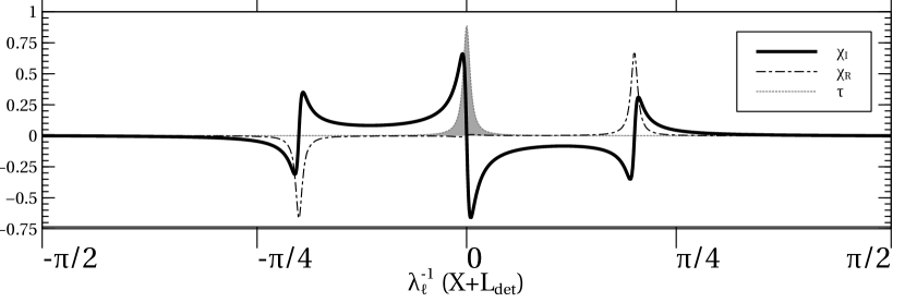
Figure 1: The PDH signal $\chi$ for a resonant cavity, as a function of the phase shift $\lambda_{\ell}^{-1}(X+L_{det})$. In this particular case $r_{1}=0.99$, $r_{2}=0.98$ and $L_{0}=1\mathrm{m}$, which gives a free spectral range of $f_{FSR}=150\mathrm{MHz}$. The modulation frequency is $f_{m}=(2\pi)^{-1}\omega_{m}=30\mathrm{MHz}$. The continuous line is the imaginary part $\chi_{I}=\mbox{Im}\,\chi$ of the PDH signal, the dotted line its real part $\chi_{R}=\mbox{Re}\,\chi$. The dotted filled graph is the ratio $\tau$ between the transmitted intensity and the input one.

The phase shift induced by the cavity can be measured with the Pound Drever Hall technique (PDH, ; PDHpedagogical, ), which gives a complex signal $\chi$ that can be written as

$$\chi\equiv\chi_{R}+i\chi_{I}={\cal R}\left(\phi\right){\cal R}\left(\phi_{+}\right)^{*}-{\cal R}\left(\phi\right)^{*}{\cal R}\left(\phi_{-}\right)$$ (19)

and $\phi_{\pm}=c^{-1}\left(\omega_{\ell}\pm\omega_{m}\right)\left(L_{0}+X\right)\simeq\phi\pm c^{-1}\omega_{m}L_{0}$ is the phase shift of the two PDH sidebands over the cavity length. An example of $\chi$ is given in Figure 1 for a somewhat arbitrary choice of the relevant parameters. It is evident that the connection between the cavity displacement and $\chi$ is linear only in a small interval $O\left(\lambda_{\ell}{\cal F}^{-1}\right)$ around the resonance, where it can be used as an error signal.

Another useful signal is given by the ratio between the transmitted intensity and the input one, $\tau\equiv\left|\Phi_{t}\right|^{2}/\left|\Phi_{i}\right|^{2}$, where $\Phi_{t}={\cal T}\Phi_{i}$ and

$${\cal T}=\frac{t_{1}t_{2}e^{i\phi}}{1-r_{1}r_{2}e^{2i\phi}}\simeq\frac{t_{1}t_{2}e^{i\phi}}{1-r_{1}r_{2}}\frac{1}{1+\frac{{\cal{\cal F}}}{\pi}\left(1-e^{2i\phi}\right)}\Phi_{i}$$ (20)

In order for $\tau$ to be different from zero we must allow for a (small) transmissivity $t_{2}$. This is also plotted in Figure 1: note that it can be used as a trigger, as it becomes different from zero in a significant way only in the linear region of the PDH signal.

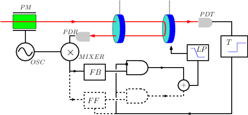
Figure 2: A schematic representation of the locking procedure. Both the light transmitted by the cavity, measured by the photodiode $PDT$, and the phase shift Pound Drever signal measured by the photodiode $PDR$ are used. The transmitted signal is used as a trigger, to discriminate between the inside LRAR and the outside LRAR regimes. Inside the LRAR a standard feedback force $FB$ is applied to the system, while outside the feed forward force $FF$ is used. The feed forward force is provided by $FF$ taking into account the value of the cavity velocity at the exit of LRAR. The low pass filter allow for a smooth transition between feedback and feed forward.

In Figure 2 we schematized the proposed improved locking strategy. The non dashed parts represent the usual locking scheme, the dashed one our additions. The two parts are activated respectively inside and outside the LRAR: in the first case we have a feed backward scheme, in the second a feed forward one.

We can assume that, up to a negligible measurement error, the state of the system will be known exiting the LRAR. The main problem for locking acquisition is the value of the velocity: if too large, the usual lock attempt will require a large feedback force. Our strategy can now be described as follows: when the cavity exit the LRAR we will stop to measure its state. But, using our knowledge of the probability distribution during the out of resonance period, we apply a feed forward force $f$ optimized in such a way to reduce the cavity speed, when it will reenter the LRAR.

In particular, suppose the exiting velocity of the cavity to be $v_{exit}>0$. The cavity can reenter the LRAR around the same resonance, with a final velocity $v<0$, or around the first one on the right, with a final velocity $v>0$. A key quantity will be the LRAR reentering velocity distribution $P_{RVD}\left(v;v_{exit}^{2},f\right)$, which is a function of $v_{exit}^{2}$ and a functional of $f$. Starting from $P_{RVD}\left(v;v_{exit}^{2},f\right)$ it will easy to evaluate the square several parameter of interest.

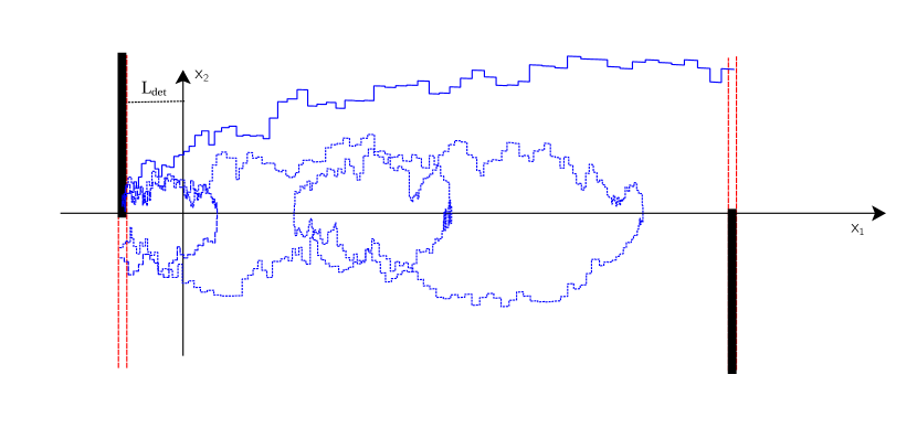
Figure 3: A sample of schematic trajectories which contribute to the LRAR reentering velocity distribution $P_{RVD}$, with the same initial velocity. The continuous line contributes to the $v>0$ part of $P_{RVD}$, the dashed and dotted lines to the $v<0$ one. Note that the noise allows the cavity to invert several time its speed before reentering in the LRAR (dotted line). For illustrative purposes the trajectories are discretized, and have been simulated as a sequence of a vertical step due to the noise and a transport one. The tick lines are the absorbing boundaries, where $P\left(\boldsymbol{x},t\mid\boldsymbol{x}_{0},t_{0}\right)=0$.

In order to calculate $P_{RVD}\left(v;v_{exit}^{2},f\right)$ we need to solve the Fokker Planck equation with peculiar boundary conditions which represent absorbing barriers at the LRARs. In Figure 3 we represented the strip of the state space between two LRAR of interest (double dashed lines) centered in $x_{1}\equiv x_{L}$ and $x_{1}\equiv x_{R}=x_{L}+\frac{\lambda_{\ell}}{2}$. When the state of the cavity enters a LRAR we want to stop to consider it, so we set $P\left(\boldsymbol{x},t\mid\boldsymbol{x}^{\prime},t^{\prime}\right)=0$ outside the strip. In our particular case there is not a diffusion current in the horizontal direction: this means that $P$ needs not to be continuous across the vertical boundaries of the strip. However the probability current on the boundaries

$$J_{1}\left(\boldsymbol{x},t\right) =\left.P\left(\boldsymbol{x},t\mid\boldsymbol{x}^{\prime},t^{\prime}\right)\boldsymbol{F}\left(\boldsymbol{x}\right)\cdot\boldsymbol{e}_{1}\right|_{x_{1}=x_{L,R}}$$

$$=\left.\omega_{0}P\left(\boldsymbol{x},t\mid\boldsymbol{x}^{\prime},t^{\prime}\right)x_{2}\right|_{x_{1}=x_{L,R}}$$

must be directed outward, and this gives the boundary conditions, valid for $t>t^{\prime}$,

$$\left.P\left(\boldsymbol{x},t\mid\boldsymbol{x}^{\prime},t^{\prime}\right)x_{2}\right|_{x_{1}=x_{L},x_{2}>0}=0$$

and

$$\left.P\left(\boldsymbol{x},t\mid\boldsymbol{x}^{\prime},t^{\prime}\right)x_{2}\right|_{x_{1}=x_{R},x_{2}<0}=0$$

which are represented by the black thick lines in Figure 3.

After finding the solution $P^{*}$ which satisfy $P^{*}\left(\boldsymbol{x},t^{\prime}\mid\boldsymbol{x}^{\prime},t^{\prime}\right)=\delta\left(\boldsymbol{x}-\boldsymbol{x}^{\prime}\right)$ with $\boldsymbol{x}^{\prime}=x_{L}\boldsymbol{e}_{1}+\omega_{0}^{-1}v_{exit}\boldsymbol{e}_{2}$ we can calculate the positive velocity part of $P_{RVD}$ as

$$P_{RVD}\left(v;v_{exit}^{2},f\right)=\left.\int_{0}^{\infty}J_{1}\right|_{x_{1}=x_{R},x_{2}=\omega_{0}^{-1}v}dt\\ =v\int_{0}^{\infty}P^{*}\left[\left(\begin{array}[]{c}x_{R}\\ \omega_{0}^{-1}v\end{array}\right),t;\left(\begin{array}[]{c}x_{L}\\ \omega_{0}^{-1}v_{exit}\end{array}\right),0\right]dt$$ (21)

and the negative velocity part as

$$P_{RVD}\left(v;v_{exit}^{2},f\right)=\left.\int_{0}^{\infty}J_{1}\right|_{x_{1}=x_{L},x_{2}=\omega_{0}^{-1}v}dt\\ =v\int_{0}^{\infty}P^{*}\left[\left(\begin{array}[]{c}x_{L}\\ \omega_{0}^{-1}v\end{array}\right),t;\left(\begin{array}[]{c}x_{L}\\ \omega_{0}^{-1}v_{exit}\end{array}\right),0\right]dt$$ (22)

As a consequence of the absorbing boundaries $P^{*}$ is not a gaussian distribution, and its normalization is not conserved: its integral over the strip at the time $t>t^{\prime}$ gives the probability for the cavity of not being reentered the LRAR at that time.

Supposing that we do not care about the particular LRAR where the system will be locked, we can design our feed forward force in such a way to maximize square velocity reduction probability

$$P_{red}\left(v_{exit}^{2},f\right)=\int_{-v_{exit}}^{v_{exit}}P_{RVD}\left(v;v_{exit}^{2},f\right)dv$$

In the best case we could obtain $P_{red}\left(v_{exit}^{2},f\right)>1/2\,\forall v_{exit}^{2}$: this would guarantees the possibility of “cooling” systematically the cavity until the locking becomes possible.

The maximization must be done over a class of functions $f$ which satisfy some set of requirements: $f$ must not be too large and with not a too large frequency bandwidth. We will write $f$ as

$$f(t)=\int_{-\infty}^{+\infty}K\left(t-t^{\prime}\right)f_{0}(t^{\prime})dt^{\prime}$$

where $\left|f_{0}(t)\right|<F_{0}$ and $K(t)$ represent a linear, time invariant, causal low pass filter.

Owing to the non trivial boundary conditions, we do not attempt here to find an analytical solution of the Fokker Planck equation, neither to determine the optimal control. Instead we evaluate numerically the performances of a set of simple control strategies:

Strategy 1

When $v_{exit}$ is large, the only option is to try to slow down the cavity until it enters the next LRAR on the right. A possible strategy is to apply the most negative constant force available $f_{0}=-F_{0}$. The real force will be given by

$$f(t)=-F_{0}g(t)$$ (23)

where $g(t)=\int_{0}^{+\infty}K(t-t^{\prime})dt^{\prime}$ is the unit step response of the filter described by $K(t)$. There are no free parameters.

Strategy 2

A second possibility, which should be effective in the intermediate region for $v_{exit}$, is to initially accelerate the cavity and then to decelerate it. This would make possible to bring the cavity to the LRAR on the right in a short time (reducing the effects of the diffusion) with a small final velocity. In this case the applied force will be

$$f(t)=F_{0}\left[g(t)-2g\left(t-\tau_{1}\right)\right]$$ (24)

with a free parameter $\tau_{1}$ to adjust.

Strategy 3

With the third strategy we attempt to bring back the cavity to its starting LRAR. This is expected to be effective for low enough values of $v_{exit}$. We need a deceleration phase followed by an acceleration one, needed to stop the typical cavity which is moving back. This gives

$$f(t)=-F_{0}\left[g(t)-2g(t-\tau_{1})\right]$$ (25)

and also in this case there is a single adjustable parameter. Note that the option Strategy 1 can be seen as the $\tau_{1}\rightarrow\infty$ limit of this one.

III.1 Numerical results

To be definite we choose a set of parameters which are somewhat representative of the typical scenario one encounter in an interferometric gravitational wave detector, setting $\omega_{0}=2\pi\,\mathrm{rad\,s^{-1}}$, $\gamma\simeq 10^{-3}\omega_{0}$ and $\lambda_{\ell}=10^{-6}\mathrm{m}$. Setting an upper frequency cut-off around $f_{c}\simeq 100\mathrm{Hz}$ for both seismic noise and control force bandwidth we have also $\tilde{\sigma}_{s}=10^{-6}/\sqrt{f_{c}}\simeq 10^{-7}\mathrm{m\,Hz^{-1/2}}$ (supposing the root mean square of seismic displacement to be $10^{-6}\mathrm{m}$). We suppose the maximal force we can apply to the mirror to be of the order of $10^{-3}\mathrm{N}$, which for a cavity mass of $\mu=20\mathrm{kg}$ gives $F_{0}=8\times 10^{-6}\mathrm{ms^{-1}}$.

It will be useful to give some order of magnitude estimates in absence of external forces. With the given parameters the length of the free cavity is spread over $\sigma_{\infty}\simeq 10^{-5}\mathrm{m}$, and its typical velocity is $\omega_{0}\sigma_{\infty}\simeq 6\times 10^{-5}\mathrm{ms^{-1}}$, which gives a typical time needed to move from a LRAR to the next one of $\tau_{T}\simeq 4\times 10^{-2}\mathrm{s}$.

Note that both $\omega_{0}\tau_{T}$ and $\gamma\tau_{T}$ are small, so we expect the details of the dynamics to be relevant only for for velocities much smaller than the typical one. In the same typical regime the relative spread of the initial velocity can be approximated as $\sigma_{v}/(\omega_{0}\sigma_{\infty})\simeq 2\sqrt{\gamma\tau_{T}}$: once again we expect diffusion effects connected to the noise to be relevant only for velocities much smaller than the typical one.

This means that when $v_{exit}$ has a typical value, or larger, we can estimate the result of the feed forward force looking only at the average value of the probability distribution. In this case by applying the first strategy we obtain always a reduction of the cavity velocity. If we have an infinitely large frequency bandwidth at our disposal then $f(t)=-F_{0}$ and the final velocity will be

$$v^{\prime}\simeq\sqrt{v_{exit}^{2}-F_{0}\lambda_{\ell}\omega_{0}}\simeq v_{exit}\left[1-\left(\frac{0.5\times 10^{-6}}{v_{exit}}\right)^{2}\right]$$

In the real case we should take into account the effect of the low pass filter impulse response $K(t)$ in Equation (23): the force will need a time $O(\omega_{c}^{-1})$ to rise to the largest value available, and the velocity reduction will be suppressed if $\omega_{c}\tau_{T}$ is small. In short, we are sure to obtain a high $P_{red}$, the velocity reduction can be small, but obviously always larger than the one obtainable in the LRAR as $\tau_{T}$ is larger compared with the time spent inside the LRAR by a factor ${\cal F}$.

What happens when $v_{exit}$ is smaller than $\omega_{0}\sigma_{\infty}$ is less obvious. In principle diffusion effect in the phase space due to the seismic noise could hamper the possibility of reducing the cavity speed.

We evaluated $P_{RVD}\left(v;v_{exit}^{2},f\right)$ by repeatedly integrating numerically the motion equations (8) with the appropriate initial position and velocity, using a simple leap frog scheme. This gives an ensemble of trajectories in the phase space (some of them are represented in Figure 3). When they reach the absorbing boundaries the integration is stopped and the final velocity is stored until a sufficient statistic is obtained.

In Figure 4 the results for the first strategy are reported. We plot the cumulative probability distribution of the ratio $\left(v/v_{exit}\right)^{2}$, for a given $v_{exit}$ which is given as a fraction of the typical one. The thick line correspond to the distribution obtained when the control force is present. For comparison the results without control force is also showed (thin line).

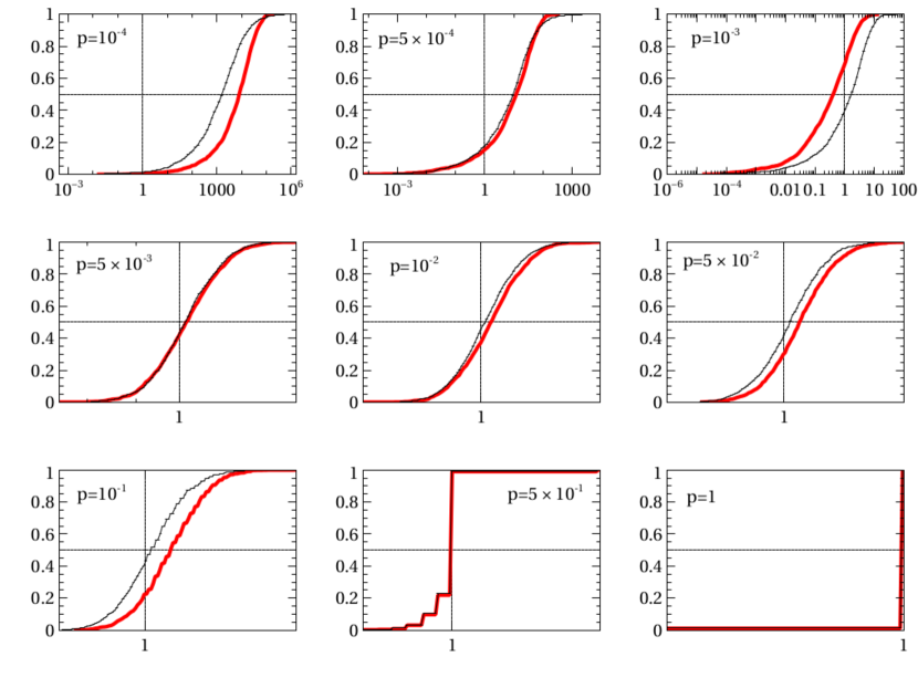
Figure 4: Results for the cumulative probability distribution of the final square velocity when the first control strategy is used, for selected values of $v_{exit}=p\omega_{0}\sigma_{\infty}$ and $F_{0}=8\times 10^{-6}\mathrm{ms^{-1}}$ (bold lines). For comparison the results with $F_{0}=0$ are also plotted (dotted lines). The value of the square velocity on the horizontal axis is normalized to the initial one.

The value of $F_{0}$ is keep constant, and we applied a third order Butterworth low pass filter. By looking at the value of the cumulative distribution when $\left(v/v_{exit}\right)^{2}=1$ we can see that we are able to obtain a velocity reduction probability larger than $1/2$ when $p=10^{-3}$.

When $p=5\times 10^{-1}$ and $p=1$ we can’t appreciate the result, because as anticipated the final velocities are almost unchanged compared with the initial one. When $p=10^{-4}$ our feedback seems to obtain a results which is the opposite of the desired one. This can be understood because in this case the cavity has a velocity which is very small compared with the typical one: the noise fluctuations accelerate it, and when we apply the control force there is a larger time available for this acceleration.

The general conclusion is that the first strategy seems to work in a specific range for $v_{exit}$. We did not attempt a full optimization at this stage.

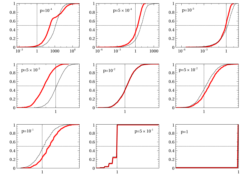
Figure 5: Results for the cumulative probability distribution of the final square velocity when the third control strategy (with $\tau_{1}=0.04\mathrm{s}$) is used, for selected values of $v_{exit}=p\omega_{0}\sigma_{\infty}$ and $F_{0}=8\times 10^{-6}\mathrm{ms^{-1}}$ (bold lines). For comparison the results with $F_{0}=0$ are also plotted (dotted lines). The value of the square velocity on the horizontal axis is normalized to the initial one.

In Figure 5 similar results are reported for the third strategy. We fixed a value for the free parameter $\tau_{1}$ which should be the optimal one in absence of fluctuations for $p=3\times 10^{-3}$. We see that we obtain the desired objective for $p=10^{-3}$ and $p=5\times 10^{-3}$, which is in agreement with the expectations. We did not attempt a full investigation in this case neither, but we expect that with an appropriate tuning of $\tau_{1}$, and with an appropriate use of the second strategy when needed, it should be possible to slow down the cavity whatever its initial velocity will be.

IV Conclusions and perspectives

We proposed a simple generalization of the common scheme used for the lock acquisition, giving some initial numerical evidence that the generalized scheme could get better performances. The discussed strategy is “blind”, in the sense that the additional control force applied to the cavity when it is outside the resonance region is a feed forward one, designed using only the last known value of the state variables and the information about the cavity dynamics. Several details have been neglected in this paper: we aimed only to discuss the basic principles, and a detailed experimental understanding is needed to discover potentially weak points.

There are however a couple of improvements that can be foreseen, and will be the object of further investigation.

IV.1 Improving the model

Our model of the cavity dynamics is quite simple. In a real situation, the mirrors are suspended to a complex attenuation system needed to reduce external seismic noise at the desired level. This means that the simple oscillator considered in this paper should be substituted by a chain of coupled ones. And, as mentioned initially, the model for the dissipation is a rough one.

In a similar way, we modeled the seismic noise in the frequency band of interest as white noise, while in a realistic scenario it will have non trivial spectral peculiarities, namely it will be a colored gaussian noise process.

We do not expect these neglected details to have a big impact on the results. As a matter of fact, during its permanence between the small region between two LRARs it will be quite a good approximation to neglect completely the dependence of the mechanical force from the position.

The specific dissipation model can have a larger impact: in the viscous case dissipation effects will be larger at higher velocity compared with structural ones, so the estimation of the efficiency of the feed forward strategy can be different. And in principle strong spectral peculiarities of the seismic noise, introducing time correlations, can make some difference.

All these are modelization issues, that can lead to the introduction of some unknown parameters. We stress that also in our simplified model there are some parameters which are totally unknown (such as $L_{det}$) or known with some uncertainty ($\gamma$, $\omega_{0}$).

In our initial discussion we introduced the prediction step described by Equation (5) and the update step described by Equation (6). In designing the feed forward scheme we used the prediction step only, but the update one play an important role when we need to cope with some unknown or partially known parameters $\boldsymbol{p}$. The basic idea is to redefine the state variables writing

$$\boldsymbol{x}^{ext}=\left(\begin{array}[]{c}\boldsymbol{x}\\ \boldsymbol{p}\end{array}\right)$$

where the dimension of $\boldsymbol{x}$ can be larger than two to accommodate a more refined mechanical model (a suspension chain, a realistic damping mechanism). The motion equation for $\boldsymbol{x}$ will depend parametrically by the variables $\boldsymbol{p}$: now we can consider the extended probability distribution $P\left(\boldsymbol{x},\boldsymbol{p},t\mid\cdots\right)$ and write a Fokker Planck equation for it.

A first possibility is to impose a trivial dynamic for $\boldsymbol{p}$ (no evolution at all) and to start from a given prior which describes our ignorance of the $\boldsymbol{p}$’s values. After each prediction step the evolved $P\left(\boldsymbol{x},\boldsymbol{p},t\mid\cdots\right)$ will be compared with a new measurement during the update step, which will select the regions of the probability space which better represent the real system.

If needed we can add a diffusive dynamics for the variables $\boldsymbol{p}$, with the possibility of adapting to slow drifts of the system. We mention that some of the parameters $\boldsymbol{p}^{seism}\in\boldsymbol{p}$ can be used to describe colored seismic noise $dW^{seism}$. This can be done by writing

$$dW^{seism}(t)=\int F\left(t-t^{\prime}\right)dW(t^{\prime})$$

where $F(t)$ is some parametrized filter function and $dW$ a Wiener process. Once again we can model our knowledge of seismic noise with some prior, and we can introduce a drift for $\boldsymbol{p}^{seism}$ to allow the model to adapt.

In our model we completely neglect the effect of radiation pressure. This is not a too bad approximation for our purposes, because radiation pressure effects are depressed outside the LRAR. When the radiation pressure is large we expect however residual effect at the LRAR boundary, which can have an impact on the feed forward design.

There are no problems in principle in introducing the radiation pressure in our model. An important difference is that there will not be a gaussian solution for the evolution of the cavity, as the equation of motion will be nonlinear. This is not a great complication, because also in the simplified model studied in this paper the probability distribution of interest is not gaussian, owing to the absorbing boundaries.

We mention that in principle it could be possible to compensate radiation pressure effects by looking at the transmitted signal $\tau$, which is just proportional to the laser intensity inside the cavity.

IV.2 Improving the locking strategy

A further improvement in the locking procedure performances could be obtained unblinding (at least partially) the control strategy outside the LRAR region. This would convert our feed forward procedure in a feedback one.

A possibility worth to be studied is the one of using the Kalman signal $\chi$ (and the transmission signal $\tau$) in the nonlinear region. Here the problem is not the nonlinear dependence of $\chi$ from the cavity position, but its non univocity. During the update step this leads to the generation of a non gaussian probability distribution. This can be parametrized with good accuracy as a gaussian misture, and we are led to the concept of particle filters (Gustafsson2002, ; Pitt2012, ), which can be seen as a way to parametrize a generic (not necessarily gaussian) probability distribution in the state space. This has the advantage of a simple implementation which does not requires tricky linearizations, but comes at the expense of a larger computational cost.

We are currently investigating all these issues, and we plan to report on them in a future paper.

Appendix A Explicit expression of evolution operators

We list for reference the explicit expressions of the operators which appears in the evolution equations for our system. The fundamental quantity is the exponential of the matrix $\mathbb{K}$

$$\mathbb{U}\left(t\right)\equiv e^{\mathbb{K}t}=e^{-\gamma t}\left(\begin{array}[]{cc}\cos\Omega t+\frac{\gamma}{\Omega}\sin\Omega t&\frac{\omega_{0}}{\Omega}\sin\Omega t\\ -\frac{\omega_{0}}{\Omega}\sin\Omega t&\cos\Omega t-\frac{\gamma}{\Omega}\sin\Omega t\end{array}\right)$$ (26)

where $\Omega^{2}=\omega_{0}^{2}-\gamma^{2}$. The inhomogeneous term of the covariance matrix is given by

$$\mathbb{Q}(\tau)=\sigma_{\infty}^{2}\left[\left(1-e^{-2\gamma\tau}\right)\mathbb{I}-\frac{2\gamma}{\Omega}e^{-2\gamma\tau}\sin\Omega t\,\mathbb{M}(t)\right]$$ (27)

where

$$\mathbb{M}(t)=\left(\begin{array}[]{cc}\frac{\gamma}{\Omega}\sin\Omega t+\cos\Omega t&\frac{\omega_{0}}{\Omega}\sin\Omega t\\ \frac{\omega_{0}}{\Omega}\sin\Omega t&\frac{\gamma}{\Omega}\sin\Omega t-\cos\Omega t\end{array}\right)$$

and $\mathbb{I}$ is the identity matrix.

The explicit expression of a multivariate gaussian distribution for the variable $\boldsymbol{x}$, with mean $\overline{\boldsymbol{x}}$ and covariance matrix $\mathbb{C}$ is given by

$${\cal N}\left(\boldsymbol{x};\overline{\boldsymbol{x}},\mathbb{C}\right)=\frac{1}{2\pi\sqrt{\det\mathbb{C}}}\exp\left[-\frac{1}{2}\left(\boldsymbol{x}-\overline{\boldsymbol{x}}\right)^{T}\mathbb{C}^{-1}\left(\boldsymbol{x}-\overline{\boldsymbol{x}}\right)\right]$$ (28)

Appendix B List of acronyms used

References

- (1) F. A. et al., Advanced virgo: a second-generation interferometric gravitational wave detector, Classical and Quantum Gravity 32 (2) (2015) 024001.
- (2) J. A. et al., Advanced ligo, Classical and Quantum Gravity 32 (7) (2015) 074001.
- (3) Y. Aso, Y. Michimura, K. Somiya, M. Ando, O. Miyakawa, T. Sekiguchi, D. Tatsumi, H. Yamamoto, Interferometer design of the KAGRA gravitational wave detector, Phys. Rev. D 88 (2013) 043007.
- (4) T. Corbitt, Y. Chen, F. Khalili, D. Ottaway, S. Vyatchanin, S. Whitcomb, N. Mavalvala, Squeezed-state source using radiation-pressure-induced rigidity, Phys. Rev. A 73 (2006) 023801.
- (5) R. Schnabel, J. Harms, K. A. Strain, K. Danzmann, {Squeezed light for the interferometric detection of high-frequency gravitational waves}, Classical and Quantum Gravity 21 (5) (2004) S1045–S1051.
- (6) The VIRGO Collaboration, The VIRGO suspensions, Classical and Quantum Gravity 19 (7) (2002) 1623.
- (7) J. Peterson, Observations and modeling of seismic background noise, U.S. Geol. Surv. Tech. Rept., 1993.
- (8) R. Kalman, A new approach to linear filtering and prediction problems, Transaction of the ASME – Journal of Basic Engineering (1960) 33–45.
- (9) S. M. Bozic, Digital and Kalman filtering : an introduction to discrete-time filtering and optimum linear estimation, E. Arnold, London, 1979.
- (10) P. S. Maybeck, Autonomous robot vehicles, Springer-Verlag New York, Inc., New York, NY, USA, 1990, Ch. The Kalman Filter: An Introduction to Concepts, pp. 194–204.
- (11) R. Mazo, Brownian motion : fluctuations, dynamics, and applications, Clarendon Press Oxford University Press, Oxford New York, 2002.
- (12) Here and in the following we neglect the effect of optical losses.
- (13) R. Drever, J. Hall, F. Kowalski, J. Hough, G. Ford, A. Munley, H. Ward, Laser phase and frequency stabilization using an optical resonator, Applied Physics B 31 (2) (1983) 97–105.
- (14) E. D. Black, An introduction to {P}ound-{D}rever-{H}all laser frequency stabilization, American Journal of Physics 69 (1) (2001) 79–87. .
- (15) The cavity mass is the reduced mass of its two mirrors.
- (16) F. Gustafsson, F. Gunnarsson, N. Bergman, U. Forssell, J. Jansson, R. Karlsson, P.-J. Nordlund, Particle filters for positioning, navigation, and tracking, IEEE Transactions on Signal Processing 50 (2) (2002) 425–437.
- (17) M. K. Pitt, N. Shephard, Filtering via Simulation: Auxiliary Particle Filters.