A reduced basis approach for calculation of the Bethe-Salpeter excitation energies using
low-rank tensor factorizations

Abstract

The Bethe-Salpeter equation (BSE) is a reliable model for estimating the absorption spectra in molecules and solids on the basis of accurate calculation of the excited states from first principles. This challenging task includes calculation of the BSE operator in terms of two-electron integrals tensor represented in molecular orbital basis, and introduces a complicated algebraic task of solving the arising large matrix eigenvalue problem. The direct diagonalization of the BSE matrix is practically intractable due to $O(N^{6})$ complexity scaling in the size of the atomic orbitals basis set, $N$. In this paper, we present a new approach to the computation of Bethe-Salpeter excitation energies which can lead to relaxation of the numerical costs up to $O(N^{3})$. The idea is twofold: first, the diagonal plus low-rank tensor approximations to the fully populated blocks in the BSE matrix is constructed, enabling easier partial eigenvalue solver for a large auxiliary system relying only on matrix-vector multiplications with rank-structured matrices. And second, a small subset of eigenfunctions from the auxiliary eigenvalue problem is selected to build the Galerkin projection of the exact BSE system onto the reduced basis set. We present numerical tests on BSE calculations for a number of molecules confirming the $\varepsilon$-rank bounds for the blocks of BSE matrix. The numerics indicates that the reduced BSE eigenvalue problem with small matrices enables calculation of the lowest part of the excitation spectrum with sufficient accuracy.

Key words: Bethe-Salpeter equation, Hartree-Fock equation, two-electron integrals, tensor decompositions, model reduction, reduced basis, truncated Cholesky factorization.

AMS Subject Classification: 65F30, 65F50, 65N35, 65F10

1 Introduction

In modern material science there is a growing interest to the ab initio computation of absorption spectra for molecules or surfaces of solids. Due to model limitations, the first principles DFT or the Hartree-Fock calculations do not allow reliable estimates for excitation energies of molecular structures. One of the approaches providing means for calculation of the excited states in molecules and solids is based on the solution of the Bethe-Salpeter equation (BSE) [27, 23, 25, 28, 29]. The alternative methods treat the problem by using the time-dependent DFT or Green’s function approach [30, 10, 6, 31, 25, 29]. The approximate coupled cluster calculations of electronic excitation energies by using rank decompositions have been described in [13].

The BSE model, originating from high energy physics and incorporating the many-body perturbation theory and the Green’s function formalism, governs calculation of the excited states in a self-consistent way. The BSE approach leads to the challenging computational task on the solution of the eigenvalue problem for a large fully populated matrix, that is in general non-symmetric. It is worth to note that the size of BSE matrix scales quadratically in the size of the basis set, $O(N^{2}_{b})$, used in ab initio electronic structure calculations. Hence the direct diagonalization is limited by $O(N_{b}^{6})$ complexity making the problem computationally extensive already for moderate size molecules with the size of the atomic orbitals basis set, $N_{b}\approx 100$. Furthermore, the numerical calculation of the matrix elements, based on the precomputed two-electron integrals (TEI) in the Hartree-Fock molecular orbitals basis, has the numerical cost that scales at least as $O(N_{b}^{4})$. In the case of non-periodic lattice structured compounds (e.g. nano-structures) the number of basis functions increases proportionally to the lattice size that easily leads to intractable problems even for small lattices. Hence, a procedure that relies entirely on multiplications of a governing BSE matrix with vectors is the only viable approach.

In this way, the numerical solution of the BSE eigenvalue problem introduces several computationally extensive sub-problems. The commonly used approaches for fast matrix computations are based on the use of certain specific data-sparse structures in the target matrix. Here, we do not consider the sparsity based on the truncation of small elements under the given threshold, since, in the particular case of BSE problem, it seems hardly implementable because of the highly non-regular sparsity pattern arising.

In this paper we study the new approach to the solution of the BSE spectral problem based on the model reduction via the reduced basis which is determined by the eigenvectors of a simplified system matrix of low-rank plus diagonal structure. We investigate the approximation error of the reduced basis set depending on the rank truncation parameters. The theoretical and numerical analysis of the existence of the low-rank approximation and the respective rank bounds for different matrix blocks in the BSE matrix is presented.

This approach includes the low-rank decomposition of the matrix blocks in the Bethe-Salpeter kernel using the Cholesky factorization of the two-electron integrals (TEI) [16, 15] represented in the Hartree-Fock molecular orbitals basis. The simplified block decomposition in the BSE system matrix is determined by the separation rank of order $O(N_{b})$, which enables compact storage and fast matrix-vector multiplications in the framework of iterations on a subspace for finding a small part of the spectrum. This opens the way to the rank-truncated arithmetics of the reduced complexity, $O(N_{b}^{3})$, that may gainfully complement the existing numerical approaches to the challenging BSE model.

Methods for solving partial eigenvalue problems for matrices with special sparse structure have been intensively studied in the literature, see for example, [5, 4, 20, 9, 2, 22, 21] and references therein. Brief surveys of commonly used rank-structured tensor formats can be found in [19, 18, 8] and in references therein.

The main computational tasks in the presented approach include the following steps:

• Precompute the TEI tensor in the Hartree-Fock molecular orbital basis in the form of low-rank factorization.

• Setting up matrix blocks in the BSE matrix that includes solution of the linear matrix equation with the identity plus low-rank governing matrix and low-rank right-hand side.

• Compute the low-rank approximation to the selected sub-matrices in the BSE matrix subject to the chosen threshold criteria.

• Construct the reduced basis set composed from eigenvectors corresponding to several lowest eigenstates of the rank-structured approximation to BSE matrix from the previous step.

• Project the initial BSE matrix onto the reduced basis and diagonalize the arising moderate size Galerkin matrix.

• Select the essential part in the spectrum of the projected Galerkin matrix and build the predicted excitation energies and the respective eigenstates.

The design of the efficient linear algebra algorithms for fast solution of arising large eigenvalue problems with rank-structured matrix blocks will be the topic for future work.

The rest of the paper is organized as follows. Section 2 outlines the truncated Cholesky decomposition scheme for low-rank factorization of the two-electron integrals tensor in the Hartree-Fock molecular orbitals basis, that is the building block in the construction of the BSE matrix. Section 3 describes the algebraic computational scheme for evaluation of the entries in the BSE matrix, analyses low-rank structure in the different matrix blocks and describes the reduced basis approach. We also analyze numerically the error of the commonly used simplified BSE model, the so-called Tamm-Dancoff (TDA) equation. The most numerically extensive part in computation of the BSE matrix blocks is reduced to finding the low-rank solution of the matrix equation with the diagonal plus low-rank structure in the governing matrix. Numerical tests indicate the convergence in the senior (lowest) excitation energies by increase of the separation ranks. Conclusion summarizes the main algorithmic and numerical features of the presented approach and outlines further prospects.

2 Low-rank approximation of the two-electron integrals in Hartree-Fock calculus

2.1 Cholesky decomposition of the TEI matrix

The numerical treatment of the two-electron integrals (TEI) is the main bottleneck in the numerical solution of the Hartree-Fock equation and in DFT calculations for large molecules.

Given the atomic orbitals basis set $\{g_{\mu}\}_{1\leq\mu\leq N_{b}}$, $g_{\mu}\in H^{1}(\mathbb{R}^{3})$, and the associated two-electron integrals (TEI) tensor ${\textbf{B}}=[b_{\mu\nu\lambda\sigma}]$ (see (5.5) in Appendix), the associated $N_{b}^{2}\times N_{b}^{2}$ TEI matrix over the large index set ${\cal I}\times{\cal J}$, $I=J={\cal I}_{b}\otimes{\cal I}_{b}$, with ${\cal I}_{b}:=\{1,...,N_{b}\}$,

$$B=mat({\textbf{B}})=[b_{\mu\nu;\lambda\sigma}]\in\mathbb{R}^{N_{b}^{2}\times N_{b}^{2}},$$

is obtained by matrix unfolding of a tensor ${\textbf{B}}=[b_{\mu\nu\lambda\sigma}]$. The TEI matrix $B$ is proven to be symmetric and positive definite. The optimized Hartree-Fock calculations are based on the incomplete Cholesky decomposition [1, 32, 12, 3, 26, 24], of the symmetric and positive definite matrix $B$,

$$B\approx LL^{T},\quad L\in\mathbb{R}^{N_{b}^{2}\times R_{B}},\quad R_{B}=O(N_{b}).$$ (2.1)

For this computation we apply the new Cholesky decomposition scheme, see [16, 15], where the adaptively chosen column vectors are calculated in the efficient way by using the precomputed redundancy free factorization of the TEI matrix $B$ (counterpart of the density fitting scheme). This allows the partial decoupling of the index sets $\{\mu\nu\}$ and $\{\lambda\sigma\}$.

Notice that the Cholesky factorization (2.1) can be written in the index form

$$b_{\mu\nu;\lambda\sigma}\approx\sum\limits_{k=1}^{R_{B}}L_{k}(\mu;\nu)L_{k}(\sigma;\lambda),$$ (2.2)

where the second factor corresponds to the transposed matrix $L_{k}^{T}$. Here $L_{k}=L_{k}(\mu;\nu)$, $k=1,...,R_{B}$, denotes the $N_{b}\times N_{b}$ matrix unfolding of the vector $L(:,k)$ in the Cholesky factor $L\in\mathbb{R}^{N_{b}^{2}\times R_{B}}$.

The results of various numerical experiments indicate that the truncated Cholesky decomposition with the separation rank $O(N_{b})$ ensures the satisfactory numerical precision $\varepsilon>0$ of order $10^{-5}$ – $10^{-6}$. The refined rank estimate $O(N_{b}|\log\varepsilon|)$ was observed in numerical experiments for every molecular system we considered so far [16, 15].

In the standard quantum chemical implementations in the Gaussian-type atomic orbitals basis the numerically confirmed rank bound $rank(B)\leq C_{B}N_{b}$ ($C_{B}$ is about several ones) allows to reduce the complexity of building up the Fock matrix $F$ to $O(N_{b}^{3})$, which is by far dominated by computational cost for the exchange term $K(D)$, see Appendix.

2.2 Rank estimates for TEI matrix $V$ and numerical illustrations

Given the complete set of Hartree-Fock molecular orbitals $\{C_{p}\in\mathbb{R}^{N_{b}}\}$, i.e. the column vectors in the coefficients matrix $C\in\mathbb{R}^{N_{b}\times N_{b}}$, and the corresponding energies $\{\varepsilon_{p}\}$, $p=1,2,...,N_{b}$ (see Appendix, where $\lambda_{i}$ correspond to $\varepsilon_{p}$). In commonly used notations, $\{C_{i}\}$ and $\{C_{a}\}$ denote the occupied and virtual orbitals, respectively.

For BSE calculations, one has to transform the TEI tensor ${\bf B}=[b_{\mu\nu\lambda\sigma}]$, corresponding to the initial AO basis set, to those represented in the molecular orbital (MO) basis,

$${\bf V}=[v_{iajb}]:\quad v_{iajb}=\sum\limits_{\mu,\nu,\lambda,\sigma=1}^{N_{b}}C_{\mu i}C_{\nu a}C_{\lambda j}C_{\sigma b}b_{\mu\nu,\lambda\sigma},\quad a,b,i,j\in\{1,...,N_{b}\}.$$ (2.3)

The BSE calculations make use of the two subtensors of ${\bf V}$ specified by the index sets ${\cal I}_{o}:=\{1,...,N_{orb}\}$ and ${\cal I}_{v}:=\{N_{orb}+1,...,N_{b}\}$, with $N_{orb}$ denoting the number of occupied orbitals (see Appendix). The first subtensor is defined as in the case of MP2 calculations,

$${\bf V}=[v_{iajb}]:\quad a,b\in{\cal I}_{v},\quad i,j\in{\cal I}_{o},$$ (2.4)

while the second one lives on the extended index set

$${\bf V}=[v_{turs}]:\quad r,s\in{\cal I}_{v},\quad t,u\in{\cal I}_{o}.$$ (2.5)

In the following, we shall use the notation $N_{v}=N_{b}-N_{orb},\;N_{ov}=N_{orb}N_{v}.$

Denote the associated matrix by ${V}=[v_{ia,jb}]\in\mathbb{R}^{N_{ov}\times N_{ov}}$ in case (2.4), and similar by ${V}=[v_{tu,rs}]\in\mathbb{R}^{N_{o}^{2}\times N_{v}^{2}}$ in case (2.5). The straightforward computation of the matrix $V$ by above representations makes the dominating impact to the overall numerical cost of order $O(N_{b}^{5})$ in the evaluation of the block entries in the BSE matrix. The method of complexity $O(N_{b}^{4})$ based on the low-rank tensor decomposition of the matrix $V$ was introduced in [15] (see §2.2).

It can be shown that the rank $R_{B}=O(N_{b})$ approximation to the TEI matrix $B\approx LL^{T},$ with the $N\times R_{B}$ Cholesky factor $L$, allows to introduce the low-rank representation of the tensor ${\bf V}$, and then reduce the asymptotic complexity of calculations to $O(N_{b}^{4})$, see [15]. Indeed, let $C_{m}$ be the m-th column of the coefficient matrix $C=\{C_{\mu i}\}\in\mathbb{R}^{N_{b}\times N_{b}}$. Then substitution of (2.2) to (2.3) in case (2.4) leads to

$$v_{iajb} =\sum\limits_{k=1}^{R_{B}}\sum\limits_{\mu,\nu,\lambda,\sigma=1}^{N_{b}}C_{\mu i}C_{\nu a}C_{\lambda j}C_{\sigma b}L_{k}(\mu;\nu)L_{k}(\sigma;\lambda)$$ (2.6)

$$=\sum\limits_{k=1}^{R_{B}}\left(\sum\limits_{\mu,\nu=1}^{N_{b}}C_{\mu i}C_{\nu a}L_{k}(\mu;\nu)\right)\left(\sum\limits_{\lambda,\sigma=1}^{N_{b}}C_{\lambda j}C_{\sigma b}L_{k}(\sigma;\lambda)\right)$$

$$=\sum\limits_{k=1}^{R_{B}}(C_{i}^{T}L_{k}C_{a})(C_{b}^{T}L_{k}^{T}C_{j})=\sum\limits_{k=1}^{R_{B}}(C_{i}^{T}L_{k}C_{a})(C_{j}^{T}L_{k}C_{b})^{T}.$$

Similar factorization can be derived in case (2.5). The precise formulation is given by the following lemma [15], which will be used in further considerations.

Lemma 2.1

Let the rank-$R_{B}$ Cholesky decomposition of the matrix $B$ be given by (2.1), then the matrix unfolding $V=[v_{ia;jb}]$ allows a rank decomposition with $rank(V)\leq R_{B}$. The $R_{B}$-term representation of the matrix unfolding $V=[v_{ia;jb}]$ takes a form

$$V=L_{V}L_{V}^{T},\quad L_{V}\in\mathbb{R}^{N_{ov}\times R_{B}},$$

where the column vectors are given by

$$L_{V}((i-1)N_{vir}+a-N_{orb};k)=C_{i}^{T}L_{k}C_{a},\quad k=1,...,R_{B},\;\;a\in{\cal I}_{v},\;\;i\in{\cal I}_{o}.$$

In case (2.5) we have $V=U_{V}W_{V}^{T}\in\mathbb{R}^{N_{o}^{2}\times N_{v}^{2}}$ with $U_{V}\in\mathbb{R}^{N_{o}^{2}\times R_{B}}$ and $W_{V}\in\mathbb{R}^{N_{ov}^{2}\times R_{B}}$.

Representation (2.6) indicates that it is necessary to compute and store the only $L_{V}$, $U_{V}$ and $W_{V}$ factors in the above rank-structured factorizations.

Lemma 2.1 provides the upper bounds on $rank(V)$ in the representation (2.6) which might be larger than that obtained by the $\varepsilon$-rank truncation. It can be shown that the $\varepsilon$-rank of the matrix $V$ remains of the same magnitude as those for the TEI matrix $B$ obtained by its $\varepsilon$-rank truncated Cholesky decomposition (see numerics in §3.2).

Numerical tests in [15] indicate that the singular values of the TEI matrix $B$ decay exponentially as

$$\sigma_{k}\leq Ce^{-\frac{z}{N_{b}}k},$$ (2.7)

where the constant $z>0$ depends weakly on the molecule configuration. If we define $R_{B}(\varepsilon)$ as the minimal number satisfying the condition

$$\sum\limits_{k=R_{B}(\varepsilon)+1}^{R_{B}}\sigma_{k}^{2}\leq\varepsilon^{2},$$

then estimate (2.7) leads to the $\varepsilon$-rank bound $R_{B}(\varepsilon)\leq CN_{b}|\log\varepsilon|$, which will be postulated in the following discussion.

Our goal is to justify that $R_{V}(\varepsilon)$ increases only logarithmically in $\varepsilon$, similar to the bound for $R_{B}(\varepsilon)$. To that end we introduce the SVD decomposition of the matrix $B$,

$$B=UD_{B}U^{T},\quad U\in\mathbb{R}^{N_{b}^{2}\times R_{B}},\;D_{B}\in\mathbb{R}^{R_{B}\times R_{B}},$$

which can be written in the index form

$$b_{\mu\nu;\lambda\sigma}=\sum\limits_{k=1}^{R_{B}}\sigma_{k}U_{k}(\mu;\nu)U_{k}(\sigma;\lambda),$$ (2.8)

with $U_{k}=[U_{k}(\mu;\nu)]\in\mathbb{R}^{N_{b}\times N_{b}}$ and $\|U_{k}\|_{F}=1$, $k=1,...,R_{B}$.

Lemma 2.2

For given $\varepsilon>0$, there exists a rank-$r$ approximation $V_{r}$ to the matrix $V$ such that $r\leq R_{B}(\varepsilon)$ and

$$\|V_{r}-V\|\leq CN_{b}\varepsilon|\log\varepsilon|,$$

where the constant $C$ does not depend of $\varepsilon$.

Proof. We estimate the $R_{B}(\varepsilon)$-term truncation error by using representation (2.8),

$$v_{iajb} =\sum\limits_{k=1}^{R_{B}}\sigma_{k}\sum\limits_{\mu,\nu,\lambda,\sigma=1}^{N_{b}}C_{\mu i}C_{\nu a}C_{\lambda j}C_{\sigma b}U_{k}(\mu;\nu)U_{k}(\sigma;\lambda)$$ (2.9)

$$=\sum\limits_{k=1}^{R_{B}}\sigma_{k}\left(\sum\limits_{\mu,\nu=1}^{N_{b}}C_{\mu i}C_{\nu a}U_{k}(\mu;\nu)\right)\left(\sum\limits_{\lambda,\sigma=1}^{N_{b}}C_{\lambda j}C_{\sigma b}U_{k}(\sigma;\lambda)\right)$$

$$=\sum\limits_{k=1}^{R_{B}}\sigma_{k}(C_{i}^{T}U_{k}C_{a})(C_{b}^{T}U_{k}^{T}C_{j})=\sum\limits_{k=1}^{R_{B}}\sigma_{k}(C_{i}^{T}U_{k}C_{a})(C_{j}^{T}U_{k}C_{b})^{T},$$

which can be presented in the matrix form $V=\sum\limits_{k=1}^{R_{B}}\sigma_{k}V_{k}V_{k}^{T}$, where $V_{k}(i;a)=C_{i}^{T}U_{k}C_{a}$. By definition of $R_{B}(\varepsilon)$ we have $\sum\limits_{k=R_{B}(\varepsilon)+1}^{R_{B}}\sigma_{k}^{2}\leq\varepsilon^{2}$. Hence, the error of rank-$R_{B}(\varepsilon)$ approximation defined by $V_{r}=\sum\limits_{k=1}^{R_{B}(\varepsilon)}\sigma_{k}V_{k}V_{k}^{T}$, can be bounded by

$$\|\sum\limits_{k=R_{B}(\varepsilon)+1}^{R_{B}}\sigma_{k}V_{k}V_{k}^{T}\| \leq(\sum\limits_{k=R_{B}(\varepsilon)+1}^{R_{B}}\sigma_{k}^{2})^{1/2}(\sum\limits_{k=R_{B}(\varepsilon)+1}^{R_{B}}\|V_{k}\|^{4})^{1/2}$$ (2.10)

$$\leq\varepsilon(\sum\limits_{k=R_{B}(\varepsilon)+1}^{R_{B}}\|V_{k}\|^{4})^{1/2}$$

$$\leq\varepsilon(R_{B}-R_{B}(\varepsilon))\|C\|_{{\cal I}_{o}}^{2}\|C\|_{{\cal I}_{v}}^{2},$$

taking into account that $\|U_{k}\|=1$, $k=1,...,R_{B}$, and the Frobenius norm estimate

$$\|V_{k}\|^{2}=\|V_{k}(i;a)\|_{F}^{2}=\|C_{i}^{T}U_{k}C_{a}\|_{F}^{2}\leq\|U_{k}\|^{2}\sum\limits_{i,a}\|C_{i}\|^{2}\|C_{a}\|^{2}\leq\sum\limits_{i}\|C_{i}\|^{2}\sum\limits_{a}\|C_{a}\|^{2}.$$

We suppose that $R_{B}=O(N_{b}|\log\varepsilon|)$, then the multiple of $\varepsilon|\log\varepsilon|$ in (2.10) does not depend on $\varepsilon$, that proves our lemma.   

The storage cost of these decompositions restricted to the active index set $I_{v}\times I_{o}$ amounts to $R_{V}(\varepsilon)N_{v}N_{orb}$. The complexity of straightforward computation on the active index set can be estimated by $O(R_{B}N_{b}^{2}N_{ov})$.

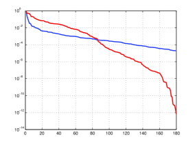
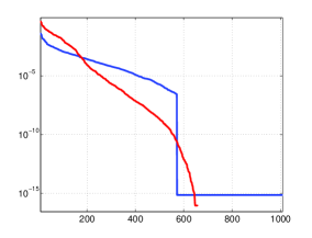
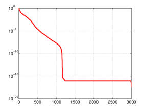
Figure 2.1: Singular values of $V$ for several moderate size molecules.

Figure 2.1 represents the singular values of the matrices $V$ (red) and $B$ (blue) for H₂O, N₂H₄, and C₂H₅NO₂ (Glycine amino acid) molecules with the size of the basis set $(N_{b},N_{orb})$ equals to $(41,9)$, $(82,9)$, and $(170,20)$, respectively. It can be seen that $R_{V}(\varepsilon)$ is linear proportional to $|\log\varepsilon|$ and it is of the same order of magnitude as $R_{B}(\varepsilon)$.

These calculations are based on the reduced truncated SVD algorithm applied to the initial Cholesky decomposition of the matrix $V$ inherited from those for the TEI matrix $B$, see Lemma 2.2 and (2.9).

3 Block tensor factorization in BSE system matrix

Here we discuss the main ingredients of the computational scheme for calculation of blocks in the BSE matrix and their reduced rank approximate representation.

3.1 Tensor representations using TEI matrix in MTO basis

The construction of BSE matrix includes computation of several auxiliary quantities. First, introduce a fourth order diagonal ”energy” matrix by

$$\boldsymbol{\Delta\varepsilon}=[\Delta\varepsilon_{ia,jb}]\in\mathbb{R}^{N_{ov}\times N_{ov}}:\quad\Delta\varepsilon_{ia,jb}=(\varepsilon_{a}-\varepsilon_{i})\delta_{ij}\delta_{ab},$$

that can be represented in the Kronecker product form

$$\boldsymbol{\Delta\varepsilon}=I_{o}\otimes\mbox{diag}\{\varepsilon_{a}:a\in{\cal I}_{v}\}-\mbox{diag}\{\varepsilon_{i}:i\in{\cal I}_{o}\}\otimes I_{v},$$

where $I_{o}$ and $I_{v}$ are the identity matrices on respective index sets. It is worth to note that if the so called homo lumo gap of the system is positive, i.e.

$$\varepsilon_{a}-\varepsilon_{i}>\delta>0,\quad a\in{\cal I}_{v},i\in{\cal I}_{o},$$

then the matrix $\boldsymbol{\Delta\varepsilon}$ is invertible.

Using the matrix $\boldsymbol{\Delta\varepsilon}$ and the $N_{ov}\times N_{ov}$ two-electron integrals matrix ${V}=[v_{ia,jb}]$ represented in the MO basis as in (2.3), the dielectric function ($N_{ov}\times N_{ov}$ matrix) $Z=[z_{pq,rs}]$ is defined by

$$z_{pq,rs}:=\delta_{pr}\delta_{qs}-v_{pq,rs}[\boldsymbol{\chi}_{0}(\omega=0)]_{rs,rs},$$

with $\boldsymbol{\chi}_{0}(\omega)$ being the matrix form of the so-called Lehmann representation to the response function. In turn, the matrix representation of $\boldsymbol{\chi}_{0}(\omega)$ inverse in known to have a form

$$\boldsymbol{\chi}_{0}^{-1}(\omega)=-\begin{pmatrix}\boldsymbol{\Delta\varepsilon}&{\bf 0}\\ {\bf 0}&\boldsymbol{\Delta\varepsilon}\\ \end{pmatrix}+\omega\begin{pmatrix}\boldsymbol{1}&{\bf 0}\\ {\bf 0}&-\boldsymbol{1}\\ \end{pmatrix},$$

implying

$$\boldsymbol{\chi}_{0}(0)=-\begin{pmatrix}\boldsymbol{\Delta\varepsilon}^{-1}&{\bf 0}\\ {\bf 0}&\boldsymbol{\Delta\varepsilon}^{-1}\\ \end{pmatrix}.$$

Let ${\bf 1}\in\mathbb{R}^{N_{ov}}$ and ${\bf d}_{\varepsilon}=\mbox{diag}\{\boldsymbol{\Delta\varepsilon}^{-1}\}\in\mathbb{R}^{N_{ov}}$ be the all-ones and diagonal vectors of $\boldsymbol{\Delta\varepsilon}^{-1}$, respectively, specifying the rank-$1$ matrix ${\bf 1}\otimes{\bf d}_{\varepsilon}$. In this notations the matrix $Z=[z_{pq,rs}]$ takes a compact form

$$Z=I_{o}\otimes I_{v}+V\odot\left({\bf 1}\cdot{\bf d}_{\varepsilon}^{T}\right),$$

where $\odot$ denotes the Hadamard product of matrices. Introducing the inverse matrix $Z^{-1}$, we finally, define the so-called static screened interaction matrix (tensor) by

$${W}=[w_{pq,rs}]:\quad w_{pq,rs}:=\sum\limits_{t\in{\cal I}_{v},u\in{\cal I}_{o}}z^{-1}_{pq,tu}v_{tu,rs}.$$ (3.1)

In the forthcoming calculations this equation should be considered on the conventional and extended index sets $\{p,s\in{\cal I}_{o}\}\cup\{q,r\in{\cal I}_{v}\}$, and $\{p,q\in{\cal I}_{o}\}\cup\{r,s\in{\cal I}_{v}\}$, respectively, corresponding to subtensors in (2.4) and in (2.5).

Hence, on the conventional index set, we obtain the following matrix factorization of $W:=[w_{ia,jb}]$,

$$W=Z^{-1}V\quad\mbox{provided that}\quad a,b\in{\cal I}_{v},\quad i,j\in{\cal I}_{o},$$

where $V$ is calculated by (2.4), while on the index set $\{p,q\in{\cal I}_{o}\}\cup\{r,s\in{\cal I}_{v}\}$ the modified matrix ${W}=[{w}_{pq,rs}]$ is computed by (3.1) and (2.5).

Now the matrix representation of the Bethe-Salpeter equation in the $(ov,vo)$ subspace reads as the following eigenvalue problem determining the excitation energies $\omega_{n}$:

$$F\begin{pmatrix}{\bf x}_{n}\\ {\bf y}_{n}\\ \end{pmatrix}\equiv\begin{pmatrix}{A}&{B}\\ {B}^{\ast}&{A}^{\ast}\\ \end{pmatrix}\begin{pmatrix}{\bf x}_{n}\\ {\bf y}_{n}\\ \end{pmatrix}=\omega_{n}\begin{pmatrix}{I}&{0}\\ {0}&{-I}\\ \end{pmatrix}\begin{pmatrix}{\bf x}_{n}\\ {\bf y}_{n}\\ \end{pmatrix},$$ (3.2)

where the matrix blocks are defined in the index notation by

$$a_{ia,jb}:=\Delta\varepsilon_{ia,jb}+v_{ia,jb}-w_{ij,ab},$$

$$b_{ia,jb}:=v_{ia,bj}-w_{ib,aj},\quad a,b\in{\cal I}_{v},\quad i,j\in{\cal I}_{o}.$$

In the matrix form we obtain

$$A=\boldsymbol{\Delta\varepsilon}+V-\overline{W},$$

where the matrix elements in $\overline{W}=[\overline{w}_{ia,jb}]$ are defined by $\overline{w}_{ia,jb}={w}_{ij,ab}$, computed by (3.1) and (2.5). Here the diagonal plus low-rank sparsity structure in $\boldsymbol{\Delta\varepsilon}+V$ can be recognized in view of Lemma 2.1. For the matrix block $B$ we have

$$B=\widetilde{V}-\widetilde{W}={V}-\widetilde{W},$$

where the matrix $\widetilde{V}$, corresponding to the partly transposed tensor, coincides with $V$,

$$\widetilde{\bf V}=[\widetilde{v}_{iajb}]:=[v_{iabj}]=[v_{iajb}],$$

and $\widetilde{W}$ is defined by permutation $\widetilde{W}=[\widetilde{w}_{ia,jb}]=[{w}_{ib,aj}]$. In the following, we will investigate the reduced rank structure in the matrix blocks $A$ and $B$ resulted from the corresponding factorizations of $V$.

Solutions of equation (3.2) come in pairs: excitation energies $\omega_{n}$ with eigenvectors $({\bf x}_{n},{\bf y}_{n})$, and de-excitation energies $-\omega_{n}$ with eigenvectors $({\bf x}_{n}^{\ast},{\bf y}_{n}^{\ast})$.

The block structure in matrices $A$ and $B$ is inherited from the symmetry of the TEI matrix $V$, $v_{ia,jb}=v^{\ast}_{ai,bj}$ and the matrix $W$, $w_{ia,jb}=w^{\ast}_{bj,ai}$. In particular, it is well known from the literature that the matrix $A$ is Hermitian (since $v_{ia,jb}=v^{\ast}_{jb,ia}$ and $w_{ij,ab}=w^{\ast}_{ji,ba}$) and the matrix $B$ is symmetric (since $v_{ia,bj}=v_{jb,ai}$ and $w_{ib,aj}=w_{ja,bi}$).

In the following, we confine ourself by the case of the real spin orbitals, i.e. the matrices $A$ and $B$ remain real. It is known that for the real spin orbitals and if ${A}+{B}$ and ${A}-{B}$ are positive definite, the problem can be transformed into a half-size symmetric eigenvalue equation [6]. Indeed, in this case for every eigenpair we have,

$$A{\bf x}+B{\bf y}=\omega{\bf x},\quad B{\bf x}+A{\bf y}=-\omega{\bf y},$$

implying

$$(A+B)({\bf x}+{\bf y})=\omega({\bf x}-{\bf y}),\quad(A-B)({\bf x}-{\bf y})=\omega({\bf x}+{\bf y}).$$

Now, if ${A}+{B}$ and ${A}-{B}$ are both positive definite, then the previous equations transform to

$$M{\bf z}=\omega^{2}{\bf z}\quad\mbox{with}\quad M=(A-B)^{1/2}(A+B)(A-B)^{1/2},$$ (3.3)

with respect to the normalized eigenvectors ${\bf z}=\sqrt{\omega}(A-B)^{1/2}({\bf x}+{\bf y})$. However, in this case the computation of the large fully populated matrix $(A-B)^{1/2}$ may become the bottleneck.

The dimension of the matrix in (3.2) is $2N_{o}N_{v}\times 2N_{o}N_{v}$, where $N_{o}$ and $N_{v}$ denote the number of occupied and virtual orbitals, respectively. In general, $N_{o}N_{v}$ is asymptotically of the size $O(N_{b}^{2})$, i.e. the spectral problem (3.2) becomes computationally extensive already for moderate size molecules with $N_{b}\approx 100$. Indeed, the direct eigenvalue solver for (3.2) (diagonalization) becomes non-acceptable due to complexity scaling $O(N_{b}^{6})$. Furthermore, the numerical calculation of the matrix elements, based on the precomputed TEI integrals from the Hartree-Fock equation, has the numerical cost that scales as $O(N_{b}^{3})-O(N_{b}^{5})$ depending on how to compute the matrix $W$. Here again we propose to adapt the low-rank structure in the matrix $V$.

The most challenging computations arise in the case of lattice structured compounds, where the number of basis functions increases proportionally to the lattice size $L\times L\times L$, i.e. $N_{b}\sim n_{0}L^{3}$, that quickly leads to intractable problems even for small lattices.

3.2 Eigenvalues in an interval by the low-rank approximation

The large matrix size in equation (3.2) makes the solution of full eigenvalue problem computationally intractable even for moderate size molecules, not saying for lattice structured compounds. Hence, in realistic quantum chemical calculations of excitation energies the computation of several tens eigenpairs may be sufficient. Methods for solving partial eigenvalue problems and matrix inversion for large matrices with special sparsity pattern have been intensively studied in the literature, see for example, [22], [21] and references therein.

3.2.1 The reduced basis approach by low-rank approximation

In what following we show that the part $\boldsymbol{\Delta\varepsilon}+V$ in the matrix block $A$ has the diagonal plus low-rank (DPLR) structure, while the sub-matrix $\widetilde{V}$ in the block $B$ exhibits the low-rank approximation. Taking into account these structures we propose the special partial eigenvalue problems solver based on the use of reduced basis set obtained from as the eigenvectors of the reduced matrix that picks up only the essential part of the initial BSE matrix with the DPLR structure. The iterative solver is based on fast matrix-vectors multiplication and efficient storage of all data involved into the computational scheme. Using the reduced basis we than solve the initial problem by the Galerkin projection onto the reduced basis of moderate size.

Another direction that includes the QTT analysis of the matrices involved in order to perform the fast matrix calculations in the QTT format will be considered elsewhere.

We begin from the low-rank decomposition of the matrix $V$,

$$V\approx L_{V}L_{V}^{T},\quad L_{V}\in\mathbb{R}^{N_{ov}\times R_{V}},\quad R_{V}\leq R_{B}.$$

where the rank parameter $R_{V}=R_{V}(\varepsilon)=O(N_{b}|\log\varepsilon|)$ can be optimized depending on the truncation error $\varepsilon>0$ (see [15] and §2.2).

First, we represent all matrix blocks and intermediate matrices included in the representation of the BSE matrix by using the above decomposition and diagonal matrices as follows. The properties of the Hadamard product imply that the matrix $Z$ exhibits the representation

$$Z=I_{o}\otimes I_{v}+L_{V}L_{V}^{T}\odot\left({\bf 1}\cdot{\bf d}_{\varepsilon}^{T}\right)=I_{N_{ov}}+L_{V}(L_{V}\odot{\bf d}_{\varepsilon})^{T},$$

where the rank of the second summand does not exceed $R_{V}$. Hence the matrix inversion $Z^{-1}$ within the calculation of $Z^{-1}V$ can be computed by special algorithm applied to the DPLR structure. The alternative way to compute the product $X=Z^{-1}V$ is the iterative solution of the matrix equation

$$ZX=V,\quad\mbox{with}\quad V=L_{V}{L}_{V}^{T},$$ (3.4)

and with the DPLR matrix $Z$. The above matrix equation can be solved in a low-rank format by using preconditioned iteration with rank truncation.

The computational cost for setting up the full BSE matrix $F$ in (3.2) can be estimated by $O({N^{3}_{ov}})$, which includes the cost $O({N_{ov}}R_{B})$ for generation of the matrix $V$ and the dominating cost $O({N^{2}_{ov}}N_{orb})$ for setting up of $W$.

In the following, we rewrite spectral problem (3.2) in the equivalent form

$$F_{1}\begin{pmatrix}{\bf x}_{n}\\ {\bf y}_{n}\\ \end{pmatrix}\equiv\begin{pmatrix}{A}&{B}\\ -{B}^{\ast}&-{A}^{\ast}\\ \end{pmatrix}\begin{pmatrix}{\bf x}_{n}\\ {\bf y}_{n}\\ \end{pmatrix}=\omega_{n}\begin{pmatrix}{\bf x}_{n}\\ {\bf y}_{n}\\ \end{pmatrix}.$$ (3.5)

The main idea of the reduced basis approach proposed in this paper is as follows. Instead of solving the partial eigenvalue problem for finding of, say, $m_{0}$ eigenpairs in equation (3.5), we, first, solve the slightly simplified auxiliary spectral problem with a modified matrix $F_{0}$ obtained from $F_{1}$ by low-rank approximation of $\overline{W}$ and $\widetilde{W}$ from the matrix blocks $A$ and $B$, respectively, i.e. by transforms

$$A\mapsto A_{0}:=\boldsymbol{\Delta\varepsilon}+V-\overline{W}_{r}\quad\mbox{and}\quad B\mapsto B_{0}:={V}-\widetilde{W}_{r}.$$ (3.6)

Here we assume that the matrix $V$ is already presented in low-rank format, inherited from the Cholesky decomposition of TEI matrix.

The modified auxiliary problem reads

$$F_{0}\begin{pmatrix}{\bf u}_{n}\\ {\bf v}_{n}\\ \end{pmatrix}\equiv\begin{pmatrix}{A}_{0}&{B}_{0}\\ -{B}_{0}^{\ast}&-{A}_{0}^{\ast}\\ \end{pmatrix}\begin{pmatrix}{\bf u}_{n}\\ {\bf v}_{n}\\ \end{pmatrix}=\lambda_{n}\begin{pmatrix}{\bf u}_{n}\\ {\bf v}_{n}\\ \end{pmatrix}.$$ (3.7)

This eigenvalue problem is much simpler than those in (3.2) since now the matrix blocks $A_{0}$ and $B_{0}$ are composed by diagonal and low-rank matrices.

Having at hand the set of $m_{0}$ eigenpairs computed for the modified (reduced model) problem (3.7), $\{(\lambda_{n},\psi_{n})=(\lambda_{n},({\bf u}_{n},{\bf v}_{n})^{T})\}$, we solve the full eigenvalue problem for the reduced matrix obtained by projection of the initial equation onto the problem adapted small basis set $\{\psi_{n}\}$ of size $m_{0}$.

Define a matrix $G_{1}=\psi_{n}(:,1:m_{0})\in\mathbb{R}^{2N_{ov}\times m_{0}}$ whose columns present the vectors of reduced basis, compute the Galerkin and mass matrices by projection onto the reduced basis specified by columns in $G_{1}$,

$$M_{1}=G_{1}^{T}F_{1}G_{1},\quad S_{1}=G_{1}^{T}G_{1}\in\mathbb{R}^{m_{0}\times m_{0}},$$

and then solve the projected generalized eigenvalue problem of small size $m_{0}\times m_{0}$,

$$M_{1}Y=\gamma_{n}S_{1}Y,\quad Y\in\mathbb{R}^{m_{0}}.$$ (3.8)

The portion of small eigenvalues $\gamma_{n}$, $n=1,...,m_{0}$, is thought to be very close to the corresponding excitation energies $\omega_{n}$, ($n=1,...,m_{0}$) in the initial spectral problem (3.2). Table 3.1 illustrates that the large the size of reduced basis $m_{0}$, the better the accuracy of the lowest excitation energy $\gamma_{1}$.

$m_{0}$	$5$	$10$	$20$	$30$	$40$	$50$
H2 O	$0.025$	$0.025$	$0.14$	$0.01$	$0.01$	$0.005$
N2H4	$0.02$	$0.02$	$0.015$	$0.015$	$0.015$	$0.005$

Table 3.1: The error $|\gamma_{1}-\omega_{1}|$ vs. the size of reduced basis, $m_{0}$.

Remark 3.1

Notice that the matrix $\overline{W}$ might have rather large $\varepsilon$-rank for small values of $\varepsilon$ which increases the cost of high accuracy solutions. The results of numerical tests that follow (see Table 3.3) indicate that the rank approximation to the matrix $\overline{W}$ with the moderate rank parameter allows for the numerical error in the excitation energies of the order of few percents. Further improvement of the accuracy requires noticeable increase in the computational costs. To avoid this numerical payoff, we apply another approximation strategy in which the matrix $\overline{W}$ remains unchanged, while matrices $V$ and $\widetilde{W}$ are substituted by their low-rank approximation (see Figure 3.3).

Matrix blocks in the auxiliary equation (3.7) are obtained by rather rough $\varepsilon$-rank approximation to the initial system matrix. However, we observe much better approximations $\gamma_{n}$ from (3.8) to the exact excitation energies $\omega_{n}$ from the equation (3.2). This can be explained by the well known effect of the quadratic error behavior of eigenvalues with respect to the perturbation error in the symmetric matrix. In the situation with equation (3.3) the corresponding statement can be easily proved under mild assumptions.

Lemma 3.2

Let matrices $A$ and $B$ be real and both $A-B$ and $A+B$ be symmetric, positive definite. Suppose that the matrices in the system (3.3) are perturbed by $A\mapsto\widetilde{A}:=A+\Delta A$, $B\mapsto\widetilde{B}:=B+\Delta B$, such that $\|\Delta A\|\leq\varepsilon$ and $\|\Delta B\|\leq\varepsilon$. Then the error in the excitation energies, $\Delta\omega_{n}=\omega_{n}-\widetilde{\omega}_{n}$, is estimated by

$$|\Delta\omega_{n}|\leq C\varepsilon^{2},$$

provided that $|2\omega_{n}+\Delta\omega_{n}|\geq\delta>0$ uniformly in $\varepsilon$.

Proof. Denote by $\lambda_{n}=\omega_{n}^{2}$ and $\widetilde{\lambda}_{n}=\widetilde{\omega}_{n}^{2}$ the exact and perturbed eigenvalues in the transformed problem (3.3). This problem is symmetric, hence we have

$$|\omega_{n}^{2}-\widetilde{\omega}_{n}^{2}|=|\lambda_{n}-\widetilde{\lambda}_{n}|\leq C\varepsilon^{2},$$

implying

$$|\omega_{n}-\widetilde{\omega}_{n}|\leq\frac{C}{|\omega_{n}+\widetilde{\omega}_{n}|}\varepsilon^{2},$$

which proves the statement.   

In the particular BSE formulation based on the Hartree-Fock molecular orbitals basis, we have the slightly perturbed symmetry in the matrix blocks, i.e. Lemma 3.2 does not apply directly. However, we observe the same quadratic error decay in all numerical experiments implemented so far.

3.2.2 Numerics for the reduced basis methods

In this section we present numerical illustrations to the reduced basis approach for the BSE problem, which use the TEI tensor and molecular orbitals obtained from the solution of the Hartree-Fock equation by the 3D grid-based tensor-structured method [14, 15]. All examples below utilize the grid representation of the Galerkin basis functions from Gaussian basis sets of type cc-pDVZ. The two-electron integrals are computed in the form of low-rank Cholesky factorization by tensor-structured algorithms incorporating 1D density fitting [16].

In the following numerical tests we demonstrate on the examples of moderate size molecules that a small reduced basis set, obtained by separable approximation with the rank parameters of about several tens, allows to reveal several lowest excitation energies and respective excited states with the accuracy about $0.1$eV - $0.02$eV depending on the rank-truncation strategy. Table 3.2 represents the size of GTO basis set, $N_{b}$, and the number of molecular orbitals, $N_{orb}$, in numerical examples considered below.

	H2O	H2O2	N2H4	C2H5OH	C2H5NO2
$N_{orb}$, $N_{b}$	$5$, $41$	$9$, $68$	$9$, $82$	$13$, $123$	$20$, $170$

Table 3.2: GTO basis set size $N_{b}$ and number of molecular orbitals, $N_{orb}$, in considered examples.

	$\varepsilon$	$4\cdot 10^{-1}$	$2\cdot 10^{-1}$	$10^{-1}$	$10^{-2}$
H2O	$|\gamma_{1}-\omega_{1}|$	$10^{-2}$	$10^{-2}$	$8\cdot 10^{-3}$	$8\cdot 10^{-6}$
	$|\lambda_{1}-\omega_{1}|$	$0.35$	$0.35$	$0.31$	$4.4\cdot 10^{-4}$
	$\|F_{1}-F_{0}\|$	$1.17$	$1.17$	$8\cdot 10^{-1}$	$2\cdot 10^{-2}$
	ranks $V$,$\overline{W}$,$\widetilde{W}$	$6$, $9$, $6$	$13$, $13$, $10$	$25$, $72$, $36$	$60$, $180$, $92$
N2H4	$|\gamma_{1}-\omega_{1}|$	$1.4\cdot 10^{-2}$	$1.5\cdot 10^{-2}$	$10^{-2}$	$6\cdot 10^{-6}$
	$|\lambda_{1}-\omega_{1}|$	$0.25$	$0.25$	$0.25$	$2.8\cdot 10^{-4}$
	$\|F_{1}-F_{0}\|$	$1.8$	$1.0$	$6\cdot 10^{-1}$	$1.4\cdot 10^{-2}$
	ranks $V$,$\overline{W}$,$\widetilde{W}$	$11$, $17$, $11$	$26$, $25$, $15$	$49$, $144$, $54$	$117$, $657$, $196$
C2H5OH	$|\gamma_{1}-\omega_{1}|$	$3\cdot 10^{-2}$	$3\cdot 10^{-2}$	$1.5\cdot 10^{-2}$	$6\cdot 10^{-6}$
	$|\lambda_{1}-\omega_{1}|$	$0.29$	$0.29$	$0.27$	$3\cdot 10^{-4}$
	$\|F_{1}-F_{0}\|$	$3.0$	$1.5$	$7\cdot 10^{-1}$	$1.4\cdot 10^{-2}$
	ranks $V$,$\overline{W}$,$\widetilde{W}$	$16$, $17$, $14$	$39$, $29$, $20$	$71$, $105$, $74$	$171$, $1430$, $296$

Table 3.3: Accuracy for 1-st eigenvalue, $|\gamma_{1}-\omega_{1}|$, and norms of the difference between the exact and reduced-rank matrices, $\|F_{1}-F_{0}\|$, vs. $\varepsilon$-rank for $V$, $\overline{W}$ and $\widetilde{W}$. The BSE matrix size is given in brackets: H₂O ($360\times 360$), N₂H₄ ($1430\times 1430$), C₂H₅OH ($2860\times 2860$).

Table 3.3 demonstrates the quadratic decay of the error $|\gamma_{1}-\omega_{1}|$ in the lowest excitation energy with respect to the approximation error to the initial BSE matrix, which is controlled by a tolerance $\varepsilon$ in the rank truncation procedure applied to the BSE submatrices $V$, $\overline{W}$ and $\widetilde{W}$. The resulting $\varepsilon$-ranks for the corresponding matrices are presented for H₂O, N₂H₄ and C₂H₅OH molecules. The error for $1$st eigenvalue, $|\gamma_{1}-\omega_{1}|$, is given in Hartree (one Hartree corresponds to $27$eV). This table demonstrates that the error in the reduced basis approximation, $|\gamma_{1}-\omega_{1}|$, is at least one order of magnitude smaller than those for simplified problem, $|\lambda_{1}-\omega_{1}|$, which motivates the use of the reduced basis equation (3.8).

This effect can be also seen in Figure 3.1 demonstrating the convergence $\gamma_{n}\to\omega_{n}$ and $\lambda_{n}\to\omega_{n}$ with respect to the increasing rank parameter determining the auxiliary problem (the size of reduced basis is $m_{0}=30$).

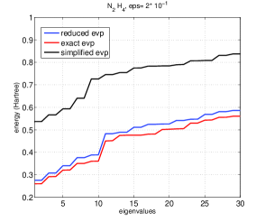
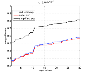
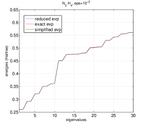
Figure 3.1: Comparison of $m_{0}=30$ lower eigenvalues for the reduced and exact BSE systems vs. $\varepsilon$ in the case of N₂H₄ molecule.

It confirms the numerical observation (see also Table 3.3) that

$$|\gamma_{n}-\omega_{n}|\ll|\lambda_{n}-\omega_{n}|,$$

that justifies the efficiency of the reduced basis approach. Three figures from the left to the right correspond to the rank truncation threshold $\varepsilon\in\{2\cdot 10^{-1}$, $10^{-1}$, $10^{-2}\}$. The quantities $\lambda_{n}$, $\gamma_{n}$ and $\omega_{n}$ are marked by black, blue and red lines, respectively. Notice that for $\varepsilon=10^{-2}$ the energies (eigenvalues) for the initial and reduced systems are practically coinciding (error of the order of $10^{-6}$), at the expense of large separation rank, see Table 3.3.

Figure 3.2 represents similar data as in Figures 3.1, but for amino-acid Glycine, C₂H₅NO₂, with the BSE matrix size $6000\times 6000$. In this case truncation threshold $\varepsilon=2\cdot 10^{-1}$ leads to the rank parameters $R_{V}=54$ , $R_{\overline{W}}=50$, $R_{\widetilde{W}}=50$, and the error for the minimal eigenvalue, $\omega_{1}=0.2432$ hartree, equals to $0.027$ hartree. For $\varepsilon=10^{-1}$ we have the rank parameters $R_{V}=100$ , $R_{\overline{W}}=215$, $R_{\widetilde{W}}=129$, and the error for the minimal eigenvalue equals to $0.014$ hartree ($0.38$eV), while the choice $\varepsilon=10^{-2}$ again ensures the accuracy of the order of $10^{-6}$.

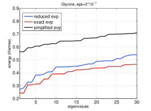
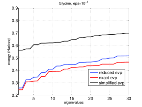
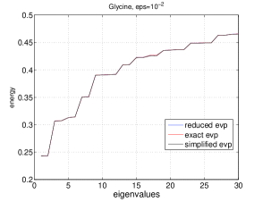
Figure 3.2: Comparison of $m_{0}=30$ lower eigenvalues for the reduced and exact BSE systems vs. $\varepsilon$ in the case of Glycine amino acid.

Figure 3.3, left, demonstrates the lowest part of the BSE spectrum corresponding to the reduced EVP in the case of a water molecule, H₂O, (rank truncation threshold $\varepsilon=10^{-1}$). The five lowest values of the computed excitation energy are approximately $8.7$eV, $10.7$eV, $11.1$eV, $12.8$eV, and $14.5$eV, see cf. [11]. Figure 3.3, center and right, illustrates the BSE energy spectrum of the H₂O molecule (based on HF calculations with cc-pDVZ-48 GTO basis) for the lowest $N_{red}=30$ eigenvalues vs. the rank truncation parameter $\varepsilon=0.6$ and $0.1$, where the ranks of $V$ and the BSE matrix block $\widetilde{W}$ are $4$, $5$ and $28$, $30$, respectively, while the block $\overline{W}$ remains unchanged. For the choice $\varepsilon=0.6$ and $\varepsilon=0.1$, the error in the 1st (lowest) eigenvalue for the solution of the problem in reduced basis is about $0.11$eV and $0.025$eV, correspondingly. The CPU time in the laptop Matlab implementation of each example is about $5$sec.

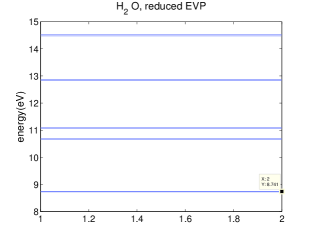
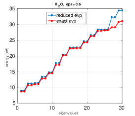
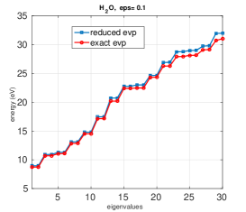
Figure 3.3: Comparison of $m_{0}=30$ lower eigenvalues for the reduced and exact BSE systems for H₂O molecule: $\varepsilon=0.6$, center; $\varepsilon=0.1$, right.

3.2.3 Comparison with the Tamm-Dancoff approximation

It is interesting to compare the full BSE model with the so-called Tamm-Dancoff approximation (TDA) [6], which corresponds to setting the matrix $B=0$ in equation (3.2). This simplifies the equation (3.2) to a standard Hermitian eigenvalue problem

$$A{\bf x}_{n}=\mu_{n}{\bf x}_{n},\quad{\bf x}_{n}\in\mathbb{R}^{N_{ov}}$$ (3.9)

with the reduced matrix size $N_{ov}$. The reduced basis approach via low-rank approximation described in §3.2.1 can be applied directly to this equation.

Below we present numerical tests indicating that the approximation error introduced by TDA method compared with the initial BSE system (3.2) remains on the level of $0.003$ hartree for several compact molecules, see Figure 3.4.

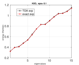
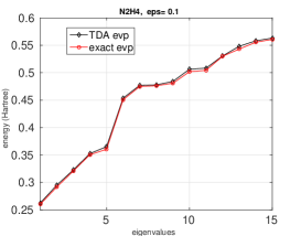
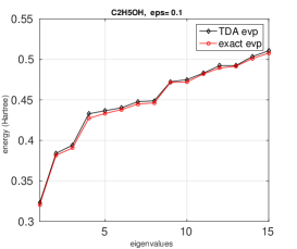
Figure 3.4: Comparison between $m_{0}=30$ lower eigenvalues $\mu_{n}$ and $\omega_{n}$ for the TDA and full BSE models, respectively, on the examples of H₂O, N₂H₄, and C₂H₅OH molecules; $\varepsilon=0.1$.

Table 3.4 indicates a tendency to decrease the TDA model error for larger molecules.

	H2O	H2O2	N2H4	C2H5OH	Glycine
err(hartree)	$0.0031$	$0.0051$	$0.0022$	$0.0024$	$0.0017$

Table 3.4: The model error $|\mu_{1}-\omega_{1}|$ in TDA approximation for different molecules, $\varepsilon=0.1$.

4 Conclusions

The new reduced basis method for solving the BSE equation based on the low-rank approximation of matrix blocks was presented and analyzed. The potential efficiency of the approach is demonstrated numerically on the solution of large scale Bethe-Salpeter eigenvalue problem for some moderate size molecules and small amino-acids. The $\varepsilon$-rank bounds for the requested sub-tensors of the TEI tensor, represented in the molecular orbitals (MO) basis set, were proven. We justify the quadratic error behavior in the excitation energies with respect to the accuracy of the rank approximation. Asymptotic estimates on the storage demands are provided.

The basic computational scheme of the reduced basis method include:

1. Precomputing step I: Given the set of Gaussian type orbitals, compute the related TEI tensor in the form of low-rank Cholesky decomposition.

2. Precomputing step II: Calculate the MO basis set and related energy spectrum by solving the Hartree-Fock eigenvalue problem.

3. Project the TEI tensor onto the MO basis set in the form of low-rank factorization.

4. Compute the diagonal plus low-rank approximations to the matrix blocks $A$ and $B$ and set up the auxiliary eigenvalue problem via rank-structured approximation to the BSE matrix.

5. Select the reduced basis set from eigenvectors corresponding to several lowest eigenstates of the auxiliary structured eigenvalue problem.

6. Compute the Galerkin projection of the exact BSE system matrix onto the reduced basis set and solve a small size reduced spectral problem by direct diagonalization.

We demonstrate that the approximation error of the reduced basis method (1) - (6) can be reduced dramatically if the matrix block $\overline{W}$ remains unchanged. We also analyze the numerical error in the simplified BSE model, the so-called Tamm-Dancoff approximation (TDA), specified by the first diagonal matrix block $A$.

The various numerical tests demonstrate that the reduced basis set obtained by solving the auxiliary eigenvalue problem based on the low-rank approximation to BSE matrix blocks (with the adaptively chosen rank parameter of the order of several tens) allows to achieve the sufficient accuracy for several lowest excited states. We justify numerically that the simplified TDA equation is characterized by the model error of the order of $0.003$ hartree ($0.08$ eV) for all molecular systems considered so far, with the tendency to decrease for large molecules, say $0.0017$ hartree ($0.045$ eV) for Glycine amino acid. We note in closing that here we mainly focus on the numerical efficiency of the new computational scheme with respect to the accuracy vs. separation rank, tested on the Hartree-Fock-BSE and Hartree-Fock-BSE-TDA calculations for some moderate size molecules.

The future work is concerned with the design of the efficient linear algebra algorithms for fast solution of arising large eigenvalue problems with diagonal plus rank-structured matrices. The approach can be also extended to the case of finite non-periodic lattice systems (e.g. quantum dots or nanoparticles) providing gainful opportunities for data-sparse matrix calculus.

Another possible direction includes the quantized tensor approximation (QTT) [17] of the matrices involved in order to perform the super-fast matrix-vector calculations in the QTT tensor arithmetics with the $\varepsilon$-rank truncation (see e.g. [7]).

Acknowledgements. The authors would like to acknowledge Prof. A. Savin (UPMC, Paris) and Prof. J. Toulouse (UPMC, Paris) for valuable comments on the problem setting for the BSE model and for providing the useful references.

5 Appendix: The Hartree-Fock model

The $2N_{orb}$-electrons Hartree-Fock equation for pairwise $L^{2}$-orthogonal electronic orbitals, $\psi_{i}:\mathbb{R}^{3}\to\mathbb{R}$, $\psi_{i}\in H^{1}(\mathbb{R}^{3})$, reads as

$${\cal F}\psi_{i}({x})=\lambda_{i}\,\psi_{i}({x}),\quad\int_{\mathbb{R}^{3}}\psi_{i}\psi_{j}dx=\delta_{ij},\;\;i,j=1,...,N_{orb},$$ (5.1)

with ${\cal F}$ being the nonlinear Fock operator

$${\cal F}:=-\frac{1}{2}\Delta+V_{c}+V_{H}+{\cal K}.$$

Here the nuclear potential takes the form

$$V_{c}(x)=-\sum_{\nu=1}^{M}\frac{Z_{\nu}}{\|{x}-a_{\nu}\|},\quad Z_{\nu}>0,\;\;a_{\nu}\in\mathbb{R}^{3},$$

while the Hartree potential $V_{H}({x})$ and the nonlocal exchange operator $\cal K$ read as

$$V_{H}({x}):=\rho\star\frac{1}{\|\cdot\|}=\int_{\mathbb{R}^{3}}\frac{\rho({y})}{\|{x}-{y}\|}\,d{y},\quad{x}\in{\mathbb{R}^{3}},$$ (5.2)

and

$$\left({\cal K}\psi\right)({x}):=-\sum_{i=1}^{N_{orb}}\left(\psi\,\psi_{i}\star\frac{1}{\|\cdot\|}\right)\psi_{i}(x)=-\frac{1}{2}\int_{\mathbb{R}^{3}}\;\frac{\tau({x},{y})}{\|{x}-{y}\|}\,\psi({y})d{y},$$ (5.3)

respectively. Conventionally, we use the definitions

$$\tau({x},{y}):=2\sum_{i=1}^{N_{orb}}\;\psi_{i}({x})\psi_{i}({y}),\quad\rho({x}):=\tau({x},{x}),\quad$$

for the density matrix $\tau({x},{y})$, and electron density $\rho({x})$.

Usually, the Hartree-Fock equation is approximated by the standard Galerkin projection of the initial problem (5.1) posed in $H^{1}(\mathbb{R}^{3})$. For a given finite Galerkin basis set $\{g_{\mu}\}_{1\leq\mu\leq N_{b}}$, $g_{\mu}\in H^{1}(\mathbb{R}^{3})$, the occupied molecular orbitals $\psi_{i}$ are represented (approximately) as

$$\psi_{i}=\sum\limits_{\mu=1}^{N_{b}}C_{\mu i}g_{\mu},\quad i=1,...,N_{orb}.$$ (5.4)

To derive an equation for the unknown coefficients matrix $C=\{C_{\mu i}\}\in\mathbb{R}^{N_{b}\times N_{orb}}$, first, we introduce the mass (overlap) matrix $S=\{S_{\mu\nu}\}_{1\leq\mu,\nu\leq N_{b}}$, given by

$$S_{\mu\nu}=\int_{\mathbb{R}^{3}}g_{\mu}g_{\nu}dx,$$

and the stiffness matrix $H=\{h_{\mu\nu}\}$ of the core Hamiltonian ${\cal H}=-\frac{1}{2}\Delta+V_{c}$ (the single-electron integrals),

$$h_{\mu\nu}=\frac{1}{2}\int_{\mathbb{R}^{3}}\nabla g_{\mu}\cdot\nabla g_{\nu}dx+\int_{\mathbb{R}^{3}}V_{c}(x)g_{\mu}g_{\nu}dx,\quad 1\leq\mu,\nu\leq N_{b}.$$

The core Hamiltonian matrix $H$ can be precomputed in $O(N_{b}^{2})$ operations via grid-based approach.

Given the finite basis set $\{g_{\mu}\}_{1\leq\mu\leq N_{b}}$, $g_{\mu}\in H^{1}(\mathbb{R}^{3})$, the associated fourth order two-electron integrals (TEI) tensor, ${\textbf{B}}=[b_{\mu\nu\lambda\sigma}]$, is defined entrywise by

$$b_{\mu\nu\lambda\sigma}=\int_{\mathbb{R}^{3}}\int_{\mathbb{R}^{3}}\frac{g_{\mu}(x)g_{\nu}(x)g_{\lambda}(y)g_{\sigma}(y)}{\|x-y\|}dxdy,\quad\mu,\nu,\lambda,\sigma\in\{1,...,N_{b}\}=:{\cal I}_{b}.$$ (5.5)

In computational quantum chemistry the nonlinear terms representing the Galerkin approximation to the Hartree and exchange operators are calculated traditionally by using the low-rank Cholesky decomposition of the TEI tensor ${\bf B}=[b_{\mu\nu\kappa\lambda}]$ as defined in (5.5), (2.1) that initially has the computational and storage complexity of order $O(N_{b}^{4})$.

Introducing the $N_{b}\times N_{b}$ matrices $J(D)$ and $K(D)$,

$$J(D)_{\mu\nu}=\sum\limits_{\kappa,\lambda=1}^{N_{b}}b_{\mu\nu,\kappa\lambda}D_{\kappa\lambda},\quad K(D)_{\mu\nu}=-\frac{1}{2}\sum\limits_{\kappa,\lambda=1}^{N_{b}}b_{\mu\lambda,\nu\kappa}D_{\kappa\lambda},$$ (5.6)

where $D=2CC^{T}\in\mathbb{R}^{N_{b}\times N_{b}}$ is the rank-$N_{orb}$ symmetric density matrix, one then represents the complete Fock matrix $F$ by

$$F(D)=H+J(D)+K(D).$$ (5.7)

The resultant Galerkin system of nonlinear equations for the coefficients matrix $C\in\mathbb{R}^{N_{b}\times N_{orb}}$, and the respective eigenvalues $\Lambda$, reads as

$$F(D)C =SC\Lambda,\quad\Lambda=diag(\lambda_{1},...,\lambda_{N_{b}}),$$ (5.8)

$$C^{T}SC =I_{N},$$

where the second equation represents the orthogonality constraints $\int_{\mathbb{R}^{3}}\psi_{i}\psi_{j}dx=\delta_{ij}$, and $I_{N}$ denotes the $N_{b}\times N_{b}$ identity matrix.

References

- [1] N. Beebe and J. Linderberg. Simplifications in the generation and transformation of two-electron integrals in molecular calculations. Int. J. Quantum Chem., (7):683–705, 1977.
- [2] P. Benner, H. Faßbender, and M. Stoll. Solving large-scale quadratic eigenvalue problems with hamiltonian eigenstructure using a structure-preserving Krylov subspace method. Electronic Transactions on Numerical Analysis, 29:212–229, 2008.
- [3] P. Benner, P. Kürschner, and J. Saak. Efficient handling of complex shift parameters in the low-rank cholesky factor adi method. Numerical Algorithms, 62(2):225–251, 2013.
- [4] P. Benner, V. Mehrmann, and H. Xu. A new method for computing the stable invariant subspace of a real Hamiltonian matrix. Journal of computational and applied mathematics, 86:17–43, 1997.
- [5] A. Bunse-Gerstner, R. Byers, and V. Mehrmann. A chart of numerical methods for structured eigenvalue problems. SIAM Journal on Matrix Analysis and Applications, (13):419–453, 1992.
- [6] M. E. Casida. Time-dependent density-functional response theory for molecules, in: Recent advances in density functional methods, part I. D.P. Chong (Ed.), World Scientific, Singapoure, 155:1207–1216, 1995.
- [7] S. Dolgov, B. Khoromskij, D. Savostyanov, and I. Oseledets. Computation of extreme eigenvalues in higher dimensions using block tensor train formats. Comp. Phys. Communications, 185(4):1207–1216, 2014.
- [8] S. V. Dolgov. Tensor product methods in numerical simulation of high-dimensional dynamical problems. PhD thesis, University of Leipzig, 2014.
- [9] H. Faßbender and D. Kressner. Structured eigenvalue problem. GAMM Mitteilungen, 29(2):297–318, 2006.
- [10] E. Gross and W. Kohn. Time-dependent density functional theory. Adv. Quant. Chem., (21):255, 1990.
- [11] A. Hermann, W. G. Schmidt, and P. Schwerdfeger. Resolving the optical spectrum of water: Coordination and electrostatic effects. Phys. Review Lett., 100:207403, 2008.
- [12] N. Higham. Analysis of the cholesky decomposition of a semi-definite matrix. In M.G. Cox and S.J. Hammarling, eds. Reliable Numerical Computations, Oxford University Press, pages 161–185, 1990.
- [13] E. G. Hohenstein, S. I. Kokkila, R. M. Parrish, and T. J. Martinez. Tensor hypercontraction equation-of-motion second-order approximate coupled cluster: electronic excitation energies in time. J. Phys. Chem., (117):12972–12978, 2013.
- [14] V. Khoromskaia. Black box Hartree-Fock solver by the tensor numerical methods. Comp. Methods in Applied Math., 14:89–111, 2014.
- [15] V. Khoromskaia and B. N. Khoromskij. Møller-Plesset (MP2) energy correction using tensor factorizations of the grid-based two-electron integrals. Comp. Phys. Communications, 185(1), 2014.
- [16] V. Khoromskaia, B. N. Khoromskij, and R. Schneider. Tensor-structured calculation of two-electron integrals in a general basis. SIAM J. Sci. Comput., 35(2), 2013.
- [17] B. N. Khoromskij. -quantics approximation of - tensors in high-dimensional numerical modeling. J. Constr. Approx., 34(2):257–289, 2011.
- [18] B. N. Khoromskij. Tensor-structured numerical methods in scientific computing: survey on recent advances. Chemometr. Intell. Lab. Syst., 110(1):1–19, 2012.
- [19] T. Kolda and B. W. Bader. Tensor decompositions and applications. SIAM Review, 51(3):455–500, 2009.
- [20] D. Kressner. Numerical methods and software for general and structured eigenvalue problems. PhD thesis, TU Berlin, Institut für Mathematik,, 2004.
- [21] L. Lin, C. Yang, J. Meza, J. Lu, L. Ying, and W. E. Selinv–an algorithm for selected inversion of a sparse symmetric matrix. ACM Transactions in Mathematical Software, 37(4), 2011.
- [22] E. Napoli, E. Polizzi, and Y. Y. Saad. Efficient estimation of eigenvalues in an interval. manuscript, 2013.
- [23] G. Onida, L. Reining, and A. Rubio. Electronic excitations: density-functional versus many-body Green’s-function approaches. Rev. of Modern Physics, 74, 2002.
- [24] R. M. Parrish, E. G. Hohenstein, N. Schunck, C. Sherrill, and T. J. Martinez. Exact tensor hypercontraction: A universal technique for the resolution of matrix elements of local finite-range N-body potentials in many-body quantum problems. Phys. Rev. Lett., (111):132505, 2013.
- [25] Y. Ping, D. Rocca, and G. Galli. Electronic excitations in light absorbers for photo-electrochemical energy conversion: first principles calculations based on many body perturbation theory. Chem. Soc. Rev., 42:2437, 2013.
- [26] S. Reine, T. Helgaker, and R. Lindh. Multi-electron integrals. WIREs Comput. Mol. Sci., (2):290–303, 2012.
- [27] L. Reining, V. Olevano, A. Rubio, and G. Onida. Excitonic effects in solids described by time-dependent density functional theory. Phys. Rev. Lett., 88:066404, 2002.
- [28] E. Ribolini, J. Toulouse, and A. Savin. Electronic excitation energies of molecular systems from the Bethe-Salpeter equation: Example of H2 molecule. In: Concepts and Methods in Modern Theoretical Chemistry (S. Ghosh and P. Chattaraj eds), vol 1: Electronic Structure and Reactivity, page 367, 2013.
- [29] E. Ribolini, J. Toulouse, and A. Savin. Electronic excitations from a linear-response range-separated hybrid scheme. Molecular Physics, 111:1219, 2013.
- [30] E. Runge and E. Gross. Density-function theory for time-dependent systems. Phys. Rev. Lett., (52):997, 1984.
- [31] R. E. Stratmann, G. E. Scuseria, and M. J. Frisch. An efficient implementation of time-dependent density-functional theory for the calculation of excitation energies of large molecules. J. Chem. Phys., 109:8218, 1998.
- [32] S. Wilson. Universal basis sets and Cholesky decomposition of the two-electron integral matrix. Comput. Phys. Commun., 58:71–81, 1990.