Impact of electromagnetism on phase structure for Wilson and twisted-mass fermions including isospin breaking

Abstract

In a recent paper we used chiral perturbation theory to determine the phase diagram and pion spectrum for Wilson and twisted-mass fermions at nonzero lattice spacing with nondegenerate up and down quarks. Here we extend this work to include the effects of electromagnetism, so that it is applicable to recent simulations incorporating all sources of isospin breaking. For Wilson fermions, we find that the phase diagram is unaffected by the inclusion of electromagnetism—the only effect is to raise the charged pion masses. For maximally twisted fermions, we previously took the twist and isospin-breaking directions to be different, in order that the fermion determinant is real and positive. However, this is incompatible with electromagnetic gauge invariance, and so here we take the twist to be in the isospin-breaking direction, following the RM123 collaboration. We map out the phase diagram in this case, which has not previously been studied. The results differ from those obtained with different twist and isospin directions. One practical issue when including electromagnetism is that the critical masses for up and down quarks differ. We show that one of the criteria suggested to determine these critical masses does not work, and propose an alternative.

I Introduction

The phase diagram of lattice QCD (LQCD) can contain unphysical transitions and unwanted phases due to discretization effects. A well known example is the Aoki phase that can be present with Wilson-like fermions Aoki (1984). Unphysical phases occur when the effects of physical light quark masses are comparable to those induced by discretization, specifically $m\sim a^{2}\Lambda_{\rm QCD}^{3}$, with $a$ the lattice spacing. This can be shown by extending chiral perturbation theory ($\chi$PT) to include the effects of discretization Sharpe and Singleton (1998). Understanding the phase structure is necessary so that LQCD simulations can avoid working close to unphysical phases, so as to avoid distortion of results and critical slowing down.

Recently, we extended the analysis of the phase diagram to the case of nondegenerate up and down quarks for Wilson-like and twisted-mass fermions Horkel and Sharpe (2014). This was prompted by the recent incorporation of mass splittings into simulations of LQCD. We found a fairly complicated phase structure, in which, for example, the Aoki phase was continuously connected to Dashen’s CP-violating phase Dashen (1971); Creutz (2004).

A drawback of our analysis was that it did not include the other major source of isospin breaking in QCD, namely electromagnetism. For most hadron properties, electromagnetic effects are comparable to those of the mass nondegeneracy $\epsilon_{q}=(m_{u}\!-\!m_{d})/2$. For example, in the neutron-proton mass difference these two effects lead to contributions of approximately $-1\;$MeV and $2.5\;$MeV, respectively. Furthermore, the recent LQCD simulations alluded to above have included both mass nondegeneracy and electromagnetism. Thus, to be directly applicable to such simulations, we must extend our analysis to include electromagnetism. This is the purpose of the present note.

We work in Wilson or twisted-mass $\chi$PT (both of which we refer to as W$\chi$PT for the sake of brevity) using a power-counting to be explained in Sec. II. At the order we work, it turns out that the inclusion of electromagnetism can be accomplished in most cases simply by shifting low-energy coefficients (LECs) in the results without electromagnetism. Thus we can take over many results from Ref. Horkel and Sharpe (2014) without further work.

One new issue concerns the simultaneous inclusion of electromagnetism and quark nondegeneracy with twisted-mass fermions. The approach we used in the absence of electromagnetism in Ref. Horkel and Sharpe (2014) (following Ref. Frezzotti and Rossi (2004)) was to apply the twist in a different direction in isospin space ($\tau_{1}$) from that in which the masses are split ($\tau_{3}$). This leads to a real quark determinant, and is the method used to simulate the $s$ and $c$ quarks using twisted-mass fermions (see, e.g., Ref. Carrasco et al. (2014)). This does not, however, generalize to include electromagnetism in a gauge-invariant way. Here, instead, we follow Ref. de Divitiis et al. (2013), and twist in the $\tau_{3}$ direction. When doing simulations, this has the disadvantage of leading to a complex quark determinant, but there are no barriers to studying the theory with $\chi$PT.

The remainder of this paper is organized as follows. We begin in Sec. II with a brief discussion of our power-counting scheme and a summary of relevant results from Ref. Horkel and Sharpe (2014). We then explain, in Sec. III, how electromagnetism changes the results of Ref. Horkel and Sharpe (2014) for the case of Wilson-like fermions. Section IV describes how to simultaneously include isospin breaking, electromagnetism and twist, while Sec. V gives our corresponding results for the phase diagram, focusing mainly on the case of maximal twist. We conclude in Sec. VI.

Two technical issues are discussed in appendices. The first concerns the renormalization factors needed to relate lattice masses to the continuum masses that appear in $\chi$PT. This issue is subtle because singlet and nonsinglet masses renormalize differently. This point was not discussed in Ref. Horkel and Sharpe (2014), and we address it in Appendix A, except that we do not include all the effects introduced by electromagnetism.

The second appendix concerns the need for charge-dependent critical masses in the presence of electromagnetism. These must be determined nonperturbatively, and various methods for doing so have been used in the literature. One of these methods, proposed in Ref. de Divitiis et al. (2013), can be implemented using partially quenched (PQ) $\chi$PT, and thus checked. This is done in App. B. We find that the method only provides one constraint on the up and down critical masses and must be supplemented by an additional condition in order to determine both.

Appendix B requires results from a $\chi$PT analysis of a theory with twisted nondegenerate charged quarks at nonzero lattice spacing and at nonvanishing $\theta_{\rm QCD}$. We provide such an analysis in a companion paper Horkel and Sharpe (2015).

II Power-counting and summary of previous work

In order to study the low-energy properties of LQCD, we must decide on the relative importance of the competing effects. The power counting that we adopt is

$$m\sim p^{2}\sim a^{2}\sim\alpha_{\rm EM}>\epsilon_{q}^{2}>ma\sim a^{3}\sim a\alpha_{\rm EM}...\,,$$ (1)

where $m$ represents either $m_{u}$ or $m_{d}$. This is the power counting adopted in Ref. Horkel and Sharpe (2014), except that electromagnetic effects are now included. This scheme only makes sense if discretization errors linear in $a$ are absent, either because the action is improved or because the $O(a)$ terms can be absorbed into a shift in the quark masses (as is the case in W$\chi$PT Sharpe and Singleton (1998)).

The explanation for the choice of leading order (LO) terms in this power-counting is as follows. Present simulations have $1/a\approx 3\;$GeV, and using this together with $\Lambda_{\rm QCD}\approx 300\;$MeV we find $a\Lambda_{\rm QCD}\approx 0.1$. Thus second order discretization effects are of relative size $(a\Lambda_{\rm QCD})^{2}\approx 0.01$. This is comparable to $\alpha_{\rm EM}$, $m_{u}/\Lambda_{\rm QCD}$ and $m_{d}/\Lambda_{\rm QCD}$ (given that $m_{u}\approx 2.5\;$MeV and $m_{d}\approx 5\;$MeV Aoki et al. (2014); Olive et al. (2014)). The results for the neutron-proton mass difference described in the Introduction are consistent with this power-counting (using the fact that $m_{u}\!-\!m_{d}\sim m_{u}\sim m_{d}$).

The choice of $\epsilon_{q}^{2}$ as the dominant subleading contribution is less obvious, and is discussed in some detail in Ref. Horkel and Sharpe (2014). The essence of the argument is that, while the $\epsilon_{q}^{2}$ terms are not necessarily numerically larger than generic $m^{2}$ terms, they give the leading contribution from quark mass differences to isospin breaking in the low-energy effective theory. For example, these contributions give rise to the CP-violating phase in the continuum analysis.

In this note we keep only terms up to and including those proportional to $\epsilon_{q}^{2}$, so that we have the leading order term of each type. We refer to this as working at LO⁺  indicating that it goes slightly beyond keeping only LO terms.

We now collect the relevant results from Ref. Horkel and Sharpe (2014) concerning the phase diagram of Wilson-like fermions in the presence of nondegeneracy. We work entirely in SU(2) W$\chi$PT, in which the chiral field is $\Sigma\in{\rm SU(2)}$. The LO⁺ chiral Lagrangian for Wilson-like fermions (whether improved or not) is

$$\mathcal{L}_{\chi} =\frac{f^{2}}{4}\operatorname{tr}\left[\partial_{\mu}\Sigma\partial_{\mu}\Sigma^{\dagger}\right]+{\cal V}_{\chi}$$ (2)

$$\mathcal{V}_{\chi} =-\frac{f^{2}}{4}\operatorname{tr}({\chi}^{\dagger}\Sigma+\Sigma^{\dagger}{\chi})-W^{\prime}[\operatorname{tr}(\hat{A}^{\dagger}\Sigma+\Sigma^{\dagger}\hat{A})]^{2}$$

$$\quad+\frac{\ell_{7}}{16}[\operatorname{tr}(\chi^{\dagger}\Sigma-\Sigma^{\dagger}\chi)]^{2}\,,$$ (3)

where $\hat{A}=2W_{0}a\mathbb{1}$ is the spurion field used to introduce lattice artifacts. This Lagrangian contains several LECs: $f\approx 92\;$MeV and $B_{0}$ from LO continuum $\chi$PT, $W_{0}$ and $W^{\prime}$ introduced by disretization errors, and $\ell_{7}$. The latter, though of next-to-leading order (NLO) in standard continuum power-counting, leads to contributions proportional to $\epsilon_{q}^{2}$ and thus we keep it in our LO+ calculation. $\ell_{7}$ is not renormalized at one-loop order, and matching with SU(3) $\chi$PT leads to the estimate Gasser and Leutwyler (1985)

$$\ell_{7}=\frac{f^{2}}{8B_{0}m_{s}}\,,$$ (4)

indicating that $\ell_{7}$ is positive.

The final ingredient in Eq. (3) is $\chi=2B_{0}M$, which contains the mass matrix $M={\rm diag}(m_{u},m_{d})$, with $m_{u,d}$ renormalized masses in a mass-independent scheme. Since ${\cal L}_{\chi}$ is supposed to represent the long-distance physics of a lattice simulation close to the chiral and continuum limits, to use it we need to know the relationship between bare lattice masses and the renormalized masses. This relationship is nontrivial when using nondegenerate quarks, and is discussed in Appendix A. This point was overlooked in Ref. Horkel and Sharpe (2014).

To determine the vacuum of the theory, we must minimize the potential ${\cal V}_{\chi}$. Writing $\langle\Sigma\rangle=e^{i\theta\hat{n}\cdot\vec{\tau}}$, the potential becomes

$${\mathcal{V}_{\chi}}=-{f^{2}}\left(\widehat{m}_{q}\cos{\theta}+c_{\ell}\widehat{\epsilon}_{q}^{2}n_{3}^{2}\sin^{2}{\theta}+w^{\prime}\cos^{2}{\theta}\right)\,,$$ (5)

where

$$\widehat{m}_{q}=B_{0}(m_{u}\!+\!m_{d}),\ \widehat{\epsilon}_{q}=2B_{0}\epsilon_{q},\\ c_{\ell}=\frac{\ell_{7}}{f^{2}},\ w^{\prime}=\frac{64W^{\prime}W_{0}^{2}a^{2}}{f^{2}}.$$ (6)

Assuming $c_{\ell}>0$ [based on the estimate (4)], the resulting phase diagrams are shown in Fig. 1. The unshaded phases are continuum-like with $\lvert\cos\theta\rvert=1$. The shaded (pink) phases violate CP with

$$|n_{3}|=1,\ \ \cos\theta=\frac{\widehat{m}_{q}}{2(c_{\ell}\widehat{\epsilon}_{q}^{2}-w^{\prime})}.$$ (7)

The boundaries between continuum-like and CP-violating phases lie along the lines $|\widehat{m}_{q}|=2(c_{\ell}\widehat{\epsilon}_{q}^{2}-w^{\prime})$, and are second order transitions. The boundary between the two continuum-like phases with opposite $\cos\theta$ is a first order transition. Within the continuum-like phases the pion masses are

$$m_{\pi^{0}}^{2}=|\widehat{m}_{q}|-2(c_{\ell}\widehat{\epsilon}_{q}^{2}-w^{\prime})\,,\ \ m_{\pi^{\pm}}^{2}=|\widehat{m}_{q}|+2w^{\prime}\,,$$ (8)

while within the CP-violating phase

$$m_{\pi^{0}}^{2}=2(c_{\ell}\widehat{\epsilon}_{q}^{2}-w^{\prime})\sin^{2}\theta\,,\ \ m_{\pi^{\pm}}^{2}=2c_{\ell}\widehat{\epsilon}_{q}^{2}\,.$$ (9)

The neutral pion mass vanishes along the second order transition lines. Plots of these masses are given in Ref. Horkel and Sharpe (2014).

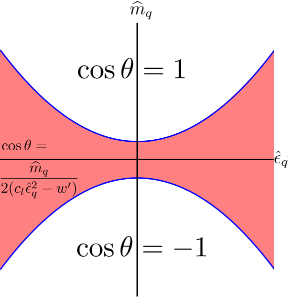
(a) Aoki scenario ($w^{\prime}<0$).

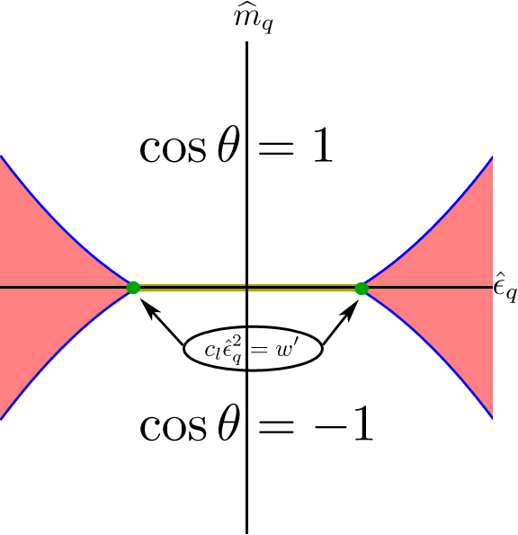
(b) First-order scenario ($w^{\prime}>0$).

Figure 1: Phase diagrams from Ref. Horkel and Sharpe (2014) including effects of both discretization and nondegenerate quarks. CP is violated in the (pink) shaded regions. The (blue) lines at the boundaries of the shade regions are second-order transitions (where the neutral pion mass vanishes), while the (yellow) line along the $\epsilon_{q}$ axis joining the two shaded regions in (1(b)) is a line of first order transitions. The analytic expression given for the shaded region in (1(a)) holds also for that in (1(b)). As discussed below in Sec. III.2, these phase diagrams apply also in the presence of electromagnetism.

III Charged, nondegenerate Wilson quarks

We now add electromagnetism, so that we are considering Wilson fermions with charged, nondegenerate quarks. Precisely how electromagnetism is added at the lattice level is not relevant; all we need to know is that electromagnetic gauge invariance is maintained by coupling to exact vector currents of the lattice theory. We work here only at LO in $\alpha_{\rm EM}$, which in terms of Feynman diagrams means keeping only those with a single photon propagator. We also work at infinite volume, thus avoiding the complications of power-law volume dependence that occur in simulations Hayakawa and Uno (2008); Davoudi and Savage (2014); Borsanyi et al. (2015).

III.1 Induced shifts in quark masses

The dominant effect of electromagnetism is a charge dependent shift in the critical mass, as noted in Refs. Portelli et al. (2010); de Divitiis et al. (2013); Borsanyi et al. (2015). Here we discuss this shift from the viewpoint of the Symanzik low-energy effective Lagrangian Symanzik (1983a, b). It arises from QCD self-energy diagrams in which one of the gluons is replaced by a photon, and leads to the appearance of the operators

$$(a) \frac{\alpha_{\rm EM}}{a}(\sum_{f}e_{f}^{2}\overline{f}f)\,,$$

$$(b) \frac{\alpha_{\rm EM}}{a}(\sum_{f^{\prime}}e_{f^{\prime}})\sum_{f}e_{f}\overline{f}f\,,$$

$$(c) \frac{\alpha_{\rm EM}}{a}\sum_{f^{\prime}}(e_{f^{\prime}}^{2})\sum_{f}\overline{f}f\,,$$ (10)

where $f=u,d$, $e_{u}=2/3$ and $e_{d}=-1/3$. Examples of the corresponding Feynman diagrams are shown in Fig. 2

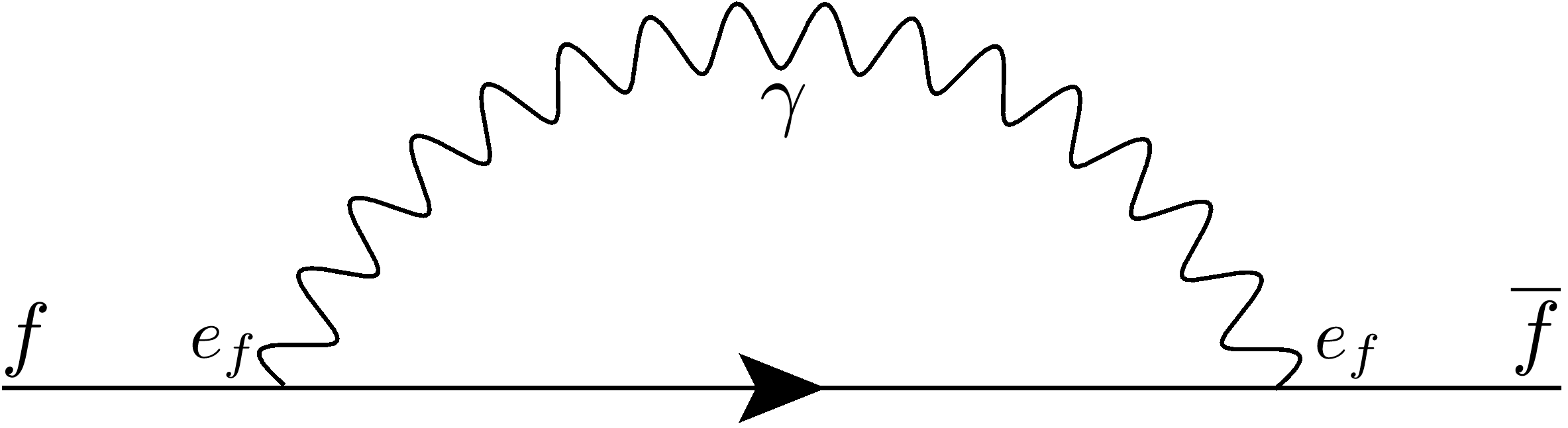
(a)

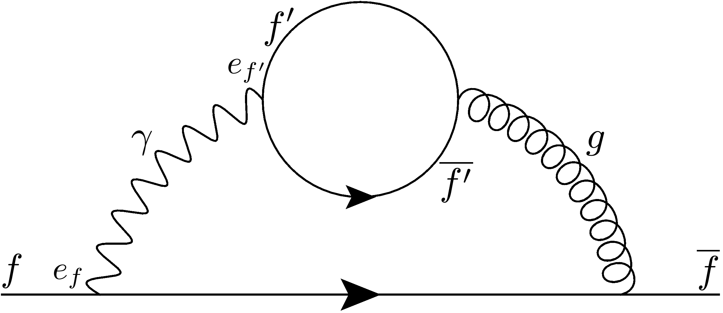
(b)

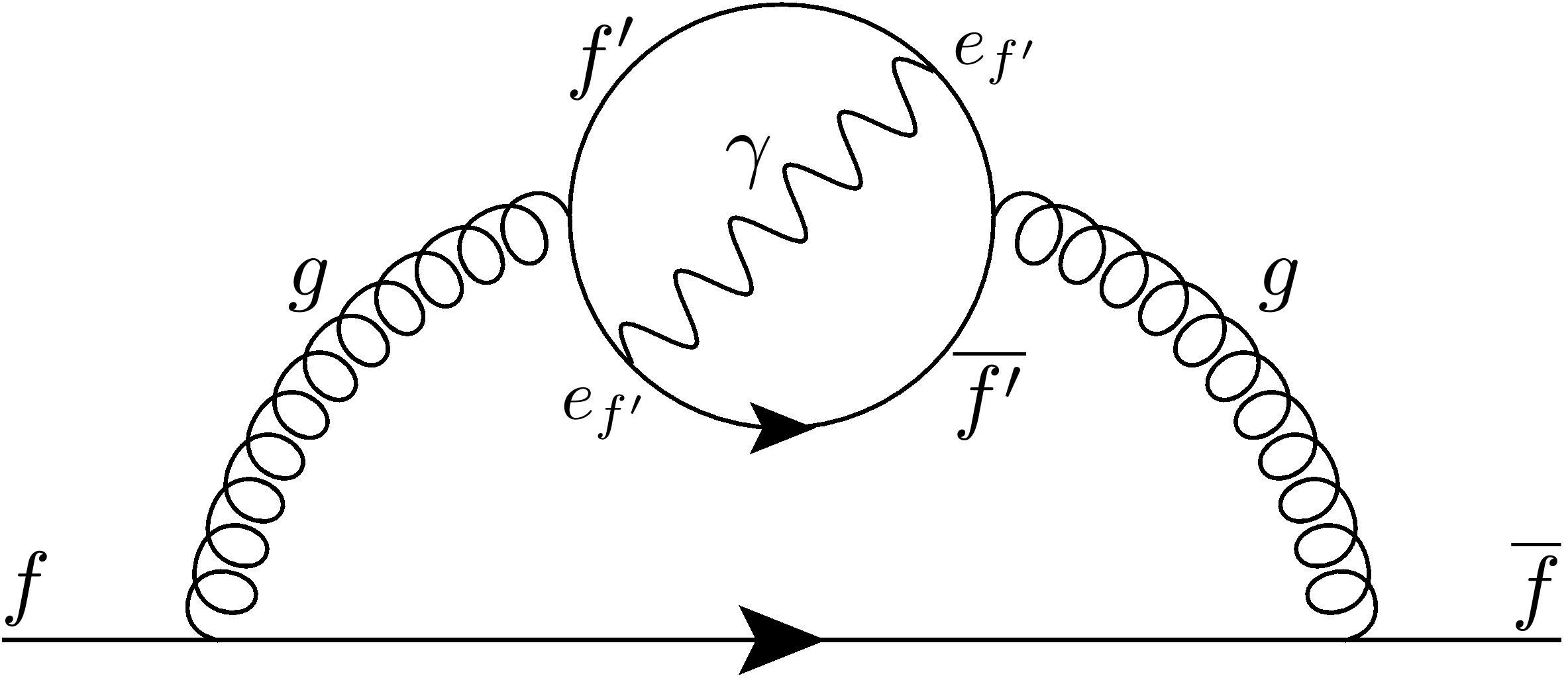
(c)

Figure 2: Examples of LO contributions from electromagnetism to quark self-energies. Diagrams with additional gluons and quark loops are not shown. These three types of diagram lead, respectively, to the three operators listed in Eq. 10. Only the first operator is present in the “electroquenched” approximation.

These operators are allowed because electromagnetism breaks isospin, while Wilson fermions violate chiral symmetries. Their contributions are smaller than those of the $\sum_{f}\bar{f}f/a$ operator that leads to the dominant shift in the critical mass. However, because $\alpha_{\rm EM}\sim a^{2}\sim m$ in our power-counting, $\alpha_{\rm EM}/a$ effects are proportional to $a\sim m^{1/2}$, and thus dominate over physical quark masses. They must therefore be removed by appropriate tuning of the bare masses. Since the combined effect of the three operators is independent ${\cal O}(\alpha_{\rm EM}/a)$ shifts in $m_{u}$ and $m_{d}$, removing these shifts requires independent tuning of the $u$ and $d$ critical masses.

Different methods for doing this tuning have been used in the literature. The most straightforward, used in Ref. Borsanyi et al. (2015), is to determine the bare quark masses directly by enforcing that an appropriate subset of hadron masses agree with their experimental values (keeping all isospin breaking effects). This avoids the need to directly determine the critical masses, but is the most challenging numerically. An alternative approach, proposed in Ref. de Divitiis et al. (2013), makes use of a partially-quenched extension of the theory. In Appendix B we check this method by showing how it can be implemented in $\chi$PT. We find that it cannot determine both critical masses, but instead only provides a single constraint between them. We then introduce an additional tuning criterion which, together with that of Ref. de Divitiis et al. (2013), does allow both critical masses to be determined.

For the rest of the main text, we assume that the charge-dependent critical masses have been determined in some manner, such that ${\cal O}(\alpha_{\rm EM}/a)$ self-energy effects can be ignored. This leaves electromagnetic corrections proportional to $\alpha_{\rm EM}$, which we must keep in our power counting, as well as higher-order effects proportional to $\alpha_{\rm EM}\times m$ etc., which we can ignore.

Examples of the latter effects are the bilinears

$$\alpha_{\rm EM}\sum_{f}e_{f}^{2}m_{f}\bar{f}f\ \ {\rm and}\ \ \alpha_{\rm EM}\sum_{f}e_{f}^{2}\bar{f}\not{D}f\,.$$ (11)

These arise as ${\cal O}(am)$ corrections to the operators of Eq. (10), and are also present directly in the continuum theory. We stress that, in the Symanzik Lagrangian, one has no dimensionful parameters other than $m$ and $1/a$, so bilinears proportional to $\alpha_{\rm EM}\Lambda_{\rm QCD}$ are not allowed. Factors of $\Lambda_{\rm QCD}$ arise when we move from the Symanzik Lagrangian to $\chi$PT.

The only effect of electromagnetism that is simply proportional to $\alpha_{\rm EM}$—and thus of LO in our power counting—is that arising from one photon exchange between electromagnetic currents. This is a continuum effect, long studied in $\chi$PT. It leads to he following additional term in the chiral potential Gupta et al. (1984); Ecker et al. (1989):

$${\cal V}_{\rm EM}=-\frac{f^{2}}{4}c_{\rm EM}\operatorname{tr}(\Sigma\tau_{3}\Sigma^{\dagger}\tau_{3})\,.$$ (12)

Here $c_{\rm EM}$ is an unknown coefficient proportional to $\alpha_{\rm EM}$. All that is known about $c_{\rm EM}$ is that it is positive Witten (1983).

III.2 Phase diagram and pion masses

The competition between electromagnetic effects and discretization errors for two degenerate Wilson fermions has been previously analyzed in Ref. Golterman and Shamir (2014). Here we add in the effects of nondegeneracy. This turns out to be very simple. Using the SU(2) identity

$$4\operatorname{tr}(\Sigma\tau_{3}\Sigma^{\dagger}\tau_{3})=\left[\operatorname{tr}(\Sigma\!+\!\Sigma^{\dagger})\right]^{2}-\left[\operatorname{tr}([\Sigma\!-\!\Sigma^{\dagger}]\tau_{3})\right]^{2}-8,$$ (13)

together with

$$\chi=\widehat{m}_{q}{\mathbb{1}}+\widehat{\epsilon}_{q}\tau_{3}\,,$$ (14)

we find that ${\cal V}_{\rm EM}$ can be absorbed into ${\cal V}_{\chi}$ [given in Eqs. (3) and (5)] by changing the existing constants as

$$w^{\prime}\longrightarrow w^{\prime}+c_{\rm EM}\,,\ \ {\rm and}\ \ c_{\ell}\widehat{\epsilon}_{q}^{2}\longrightarrow c_{\ell}\widehat{\epsilon}_{q}^{2}+c_{\rm EM}\,.$$ (15)

This allows us to determine the phase diagram and pion masses directly from the results presented in the previous section.

We first observe that, at the order we work, the phase diagram is unchanged by the inclusion of EM—the results in Fig. 1 still hold. This can be seen from the form of the potential in Eq. (5), which, since $|n_{3}|=1$, depends only on $c_{\ell}\widehat{\epsilon}_{q}^{2}-w^{\prime}$. This combination is, however, unaffected by the shifts of Eq. (15) and so the phase boundaries and values of $\theta$ throughout the phase plane are also unchanged.

Similarly, from Eqs. (8) and (9) we see that the neutral pion masses are unchanged throughout the phase plane. In particular, the second-order phase boundaries are (as expected) lines along which the neutral pion is massless.

The only change caused by electromagnetism is to the charged pion masses, which are increased by the same amount throughout the phase plane:

$$m_{\pi^{\pm}}^{2}\longrightarrow m_{\pi^{\pm}}^{2}+2c_{\rm EM}\,.$$ (16)

One implication is that, for $\widehat{\epsilon}_{q}=0$, the charged pions are no longer massless within the Aoki phase (if present). This is because they are no longer Goldstone bosons, as the flavor symmetry is explicitly broken by electromagnetism. Also, as noted in Ref. Golterman and Shamir (2014), the charged pion can be lighter than the neutral one inside the CP-violating phases. This is not inconsistent with Witten’s identity Witten (1983) because the latter did not account for discretization effects. Plots of the pion masses are shown in Fig. 3.

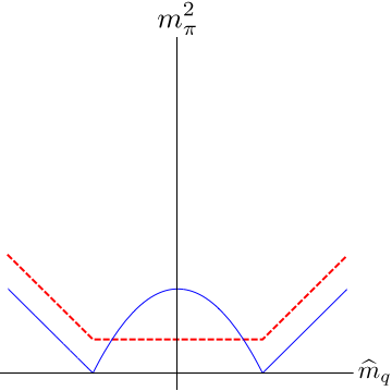
(a) Aoki scenario with $w^{\prime}<-c_{\rm EM}$

(b) First-order scenario with $w^{\prime}>c_{\ell}\widehat{\epsilon}_{q}^{2}$

(c) First-order or Aoki scenario with $-c_{\rm EM}<w^{\prime}<c_{\ell}\widehat{\epsilon}_{q}^{2}$

Figure 3: Pion masses for nondegenerate untwisted Wilson fermions including electromagnetism. The three possible behaviors along vertical slices through phase diagrams of Fig. 1 are shown. Solid (blue) lines show $m_{\pi^{0}}^{2}$, while dashed (red) lines show $m_{\pi^{\pm}}^{2}$. Expressions for masses are given in the text.

It is perhaps surprising that electromagnetism, which contributes at LO in our power-counting, has no effect on the phase diagram, whereas the subleading contributions proportional to $\widehat{\epsilon}_{q}^{2}$ have a significant impact. We can understand this by noting that the CP-violating phase is characterized by a neutral pion condensate, which remains uncoupled to the photon until higher order in $\chi$PT (where form factors enter).

The implications of these results for practical simulations (such as those of Ref. Borsanyi et al. (2015)) are unchanged from the discussion in Ref. Horkel and Sharpe (2014). In particular, for the Aoki scenario ($w^{\prime}<0$) discretization effects move the CP-violating phase closer to the physical point than for degenerate quarks, so one must beware of simulating too close to this transition.

IV Nondegeneracy, electromagnetism and twist

When using twisted-mass fermions one must decide on the relative orientation in isospin space both of the twist and the isospin-breaking induced by quark mass differences and electromagnetism. In the absence of electromagnetism, the standard choice is to align these two effects in orthogonal directions. For example, one usually takes $\tau_{3}$ for isospin-breaking, as in the continuum, while twisting in the $\tau_{1}$ direction. This is the choice used in simulations of the strange-charm sector using twisted-mass fermions Baron et al. (2011). It ensures that the fermion determinant is real, and (subject to some conditions) positive Frezzotti and Rossi (2004). This was the choice whose phase structure we determined using W$\chi$PT in Ref. Horkel and Sharpe (2014).

This approach does not, however, allow for the inclusion of electromagnetism. One problem is apparent already in the continuum limit, where the twisted-mass quark action is (in the “twisted” basis) Frezzotti et al. (2001)

$$\overline{\psi}(\not{D}+m_{q}c_{\omega}+i\gamma_{5}\tau_{1}m_{q}s_{\omega}+\epsilon_{q}\tau_{3})\psi\,.$$ (17)

Here $\not{D}$ is the gluonic covariant derivative, $m_{q}$ is the average quark mass, and $\omega$ the twist angle with $c_{\omega}=\cos\omega$ and $s_{\omega}=\sin\omega$. This action is not invariant under flavor rotations in the $\tau_{3}$ direction, so there is no conserved vector current to which the photon can couple. In other words, there is no global flavor transformation available to gauge.

To avoid this problem, we recall that twisting is, in the continuum, simply a nonanomalous change of variables that does not effect physical quantities. Thus we should start with the standard action including electromagnetism

$$\overline{\psi}(\not{D}-ie\not{A}Q+m_{q}+\epsilon_{q}\tau_{3})\psi\,,$$ (18)

with $A_{\mu}$ the photon field coupling via the charge matrix

$$Q=\frac{1}{6}{\mathbb{1}}+\frac{1}{2}\tau_{3}\,,$$ (19)

and then perform a chiral twist

$$\psi\longrightarrow e^{i\omega\gamma_{5}\tau_{1}/2}\psi,\ \ \overline{\psi}\longrightarrow\overline{\psi}e^{i\omega\gamma_{5}\tau_{1}/2}\,.$$ (20)

This leads to the quark action of Eq. (17) with the addition of the photon coupling

$$\overline{\psi}\not{A}\left[\frac{1}{6}{\mathbb{1}}+\frac{1}{2}(c_{\omega}\tau_{3}-s_{\omega}\tau_{2}\gamma_{5})\right]\psi\,.$$ (21)

Thus the photon couples to a linear combination of vector currents and to an axial current in the $\tau_{2}$ direction. In the continuum, this combination is conserved [given the twisted mass matrix of Eq. (17)] and the action remains gauge invariant.

We conclude that the correct fermion action to discretize is the sum of Eqs. (17) and (21). This, however, is not possible in a gauge invariant way using Wilson’s lattice derivative (except for $s_{\omega}=0$). The Wilson term breaks all axial symmetries, so the $\tau_{2}\gamma_{5}$ part of the photon coupling is to a lattice current that is not conserved.

To avoid this problem, and obtain a discretized twisted theory that maintains gauge invariance, one needs to twist in a direction that leaves the photon coupling to a conserved current. The only choice is to twist in the $\tau_{3}$ direction. Then the twisted form of the continuum Lagrangian is

$$\overline{\psi}(\not{D}-ie\not{A}Q+m_{q}c_{\omega}+\tau_{3}\epsilon_{q}c_{\omega}+i\gamma_{5}\tau_{3}m_{q}s_{\omega}+i\gamma_{5}\epsilon_{q}s_{\omega})\psi\,.$$ (22)

This is discretized by adding the standard Wilson term. Since the photon is coupled to vector currents that are exact symmetries of both the Wilson term and the full mass matrix, gauge invariance is retained.

This form of the twisted isospin-violating action (with $\omega=\pi/2$) is used in the recent work of Refs. de Divitiis et al. (2012, 2013). It has one major practical disadvantage—the quark determinant is complex for nonzero twist. This is true for nondegenerate masses alone, as explained in Ref. Walker-Loud and Wu (2005). Adding electromagnetism only makes the problem worse, since at the least it induces further nondegeneracy in the masses. Because the action is complex, direct simulation with present fermion algorithms is challenging. This problem is avoided in Refs. de Divitiis et al. (2012, 2013) by doing a perturbative expansion in powers of $\epsilon_{q}$ and $\alpha_{\rm EM}$. The expectation values are then evaluated in the theory with no isospin breaking, for which the fermion determinant with twisting is real and positive.

In the following section we study the phase diagram of the theory with the discretized form of the Lagrangian (22). To our knowledge, this form of the twisted theory has not previously been studied in W$\chi$PT either with nondegeneracy alone or with electromagnetism.

V $\chi$PT for charged, nondegenerate quarks with a $\tau_{3}$ twist

The conclusion of the previous section is that the twisted-mass theory whose phase diagram is of interest is that with lattice fermion Lagrangian

$$\overline{\psi}_{L}\left[{D}_{W}+m_{0}+\tau_{3}\epsilon_{0}+i\gamma_{5}\tau_{3}\mu_{0}+i\gamma_{5}\eta_{0}\right]\psi_{L}\,.$$ (23)

$\psi_{L}$ is a lattice fermion field and $D_{W}$ the lattice Dirac operator including the Wilson term (and possibly improved). $D_{W}$ is coupled to both gluons and photons, with the latter coupling to the $\tau_{3}$ vector current. The action differs from that considered (implicitly) in Sec. III only by the addition of the two mass parameters $\mu_{0}$ and $\eta_{0}$.

The four bare mass parameters in (23) are related in the continuum limit to the renormalized up and down masses, the twist angle (which is a redundant parameter) and the QCD theta angle, $\theta_{\rm QCD}$. The aim is to tune the bare parameters so that the dimension 4 part of the quark contribution to the Symanzik effective Lagrangian is given by Eq. (22) with the desired physical quark masses, for some choice of $\omega$. As for untwisted Wilson fermions the dominant effect of electromagnetism is to cause separate ${\cal O}(\alpha_{\rm EM}/a)$ shifts in the (untwisted) up and down masses. These shifts depend on twisted masses only at quadratic order, so that, to the order we work, they are identical to those for Wilson fermions. They can be determined by the methods discussed in Sec. III.1 and Appendix B. They are equivalent to independent shifts in $m_{0}$ and $\epsilon_{0}$.

After the additive shift in $m_{0}$ and $\epsilon_{0}$, all four masses in (23) must be multiplicatively renormalized in order to be related to the continuum masses in Eq. (22). As discussed in Appendix A, this requires different renormalization factors for all four masses. We assume here that these renormalizations have been carried out, so that the dimension four term in the Symanzik effective Lagrangian is given by Eq. (22) and described by the three parameters $m_{q}$, $\epsilon_{q}$ and $\omega$.

We stress that this tuning and renormalization must be carried out with sufficient accuracy. If not, instead of Eq. (22), one ends up with a similar form having different twist angles for the $m_{q}$ and $\epsilon_{q}$ parts. The parity-odd parts can then only be removed by a combined flavor nonsinglet and flavor singlet twist. Since the latter is anomalous, this corresponds to a theory with nondegenerate quark masses, electromagnetism, a twist angle and a nonvanishing $\theta_{\rm QCD}$. In other words, the theory not only has the unphysical parity violation due to twisting (which can be rotated away in the continuum limit) but also the physical parity violation induced by $\theta_{\rm QCD}$. Indeed, to analyze the tuning in $\chi$PT one needs to include a nonvanishing $\theta_{\rm QCD}$, an analysis we carry out in a companion paper Horkel and Sharpe (2015).

Assuming that the dimension-four quark Lagrangian is Eq. (22), we next investigate which higher-dimension operators are introduced into the Symanzik Lagrangian by twisting. Those operators present for Wilson fermions remain, but, as discussed in Sec. III, are all of higher order than we consider. The dominant operators introduced by twisting will violate parity, because they are linear in the parity-violating mass terms $\mu_{0}$ and $\eta_{0}$. Examples of the new operators are

$$a\eta_{0}G_{\mu\nu}\widetilde{G}_{\mu\nu}\,,\ a\eta_{0}\overline{\psi}\widetilde{G}_{\mu\nu}\sigma_{\mu\nu}\psi\,,\ {\rm and}\ a\mu_{0}\overline{\psi}\tau_{3}\widetilde{G}_{\mu\nu}\sigma_{\mu\nu}\psi\,.$$ (24)

Since we generically treat $am$ terms as being beyond LO⁺ [see Eq. (1)], we should be able to ignore these operators. However, because $\eta_{0}\sim\epsilon_{q}$ and we are treating $\epsilon_{q}$ as somewhat enhanced, one might be concerned about dropping $a\eta_{0}$ terms. In fact, the $a\eta_{0}$ operators in (24), when matched into $\chi$PT, pick up an additional factor of $m$ or $p^{2}$, and thus are unambiguously suppressed. The reason for the extra factors is that the LO representation of a flavor-singlet pseudoscalar in $\chi$PT, $\operatorname{tr}(\Sigma-\Sigma^{\dagger})$, vanishes identically. For the induced $\theta_{\rm QCD}$ term, one can also see this result by noting that it can be rotated into the isosinglet mass term, leading to a contribution proportional to $m\theta_{\rm QCD}\sim a\epsilon m$.

Proceeding in this fashion, we find that all other new operators induced by the parity-breaking masses are beyond LO⁺ in our power counting. Thus, once the requisite tuning has been done, the LO⁺ chiral effective theory for $\tau_{3}$ twisted fermions with isospin breaking is given by the same result as for Wilson fermions, i.e.

$$\frac{f^{2}}{4}\operatorname{tr}\left[\partial_{\mu}\Sigma\partial_{\mu}\Sigma^{\dagger}\right]+{\cal V}_{\chi}+{\cal V}_{\rm EM}$$ (25)

[see Eqs. (3) and (12)], except that the quark mass matrix is now twisted

$$\chi =(\widehat{m}_{q}+\widehat{\epsilon}_{q}\tau_{3})e^{i\omega\tau_{3}}\,.$$ (26)

We analyze the phase structure of this chiral theory in the next two subsections.

V.1 Phase diagram and pion masses at maximal $\tau_{3}$ twist

We begin working at maximal $\tau_{3}$ twist, which is the choice used in Refs. de Divitiis et al. (2012, 2013). In this case

$$\chi=i\widehat{m}_{q}\tau_{3}+i\widehat{\epsilon}_{q}\,,$$ (27)

and the chiral potential becomes

$$-\frac{\mathcal{V}_{\chi+{\rm EM}}}{f^{2}} =\widehat{m}_{q}n_{3}\sin{\theta}-(c_{\ell}\widehat{\epsilon}_{q}^{2}+w^{\prime})\sin^{2}\theta$$

$$\qquad\qquad+c_{\rm EM}(\cos^{2}\theta+n_{3}^{2}\sin^{2}\theta)\,,$$ (28)

up to an irrelevant constant. Since $c_{\rm EM}>0$, the right-hand side is maximized always with $|n_{3}|=1$, and we see that the $c_{\rm EM}$ term becomes a constant. Thus, once again, electromagnetism has no impact on the phase diagram. We also see that the effect of nondegeneracy can be deduced from the results for the degenerate case (studied in Refs. Munster (2004); Scorzato (2004); Sharpe and Wu (2004)) simply by shifting $w^{\prime}$.

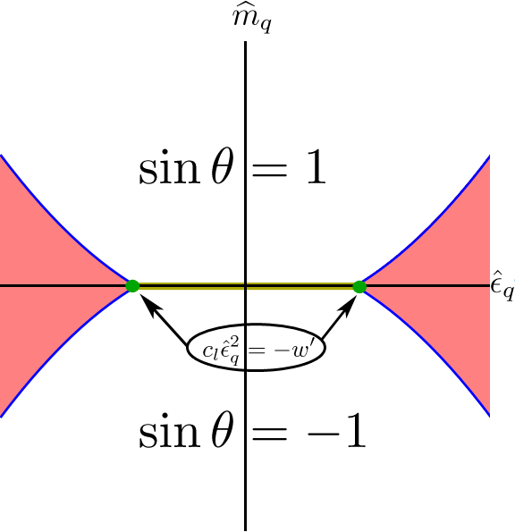
(a) Aoki scenario ($w^{\prime}<0$).

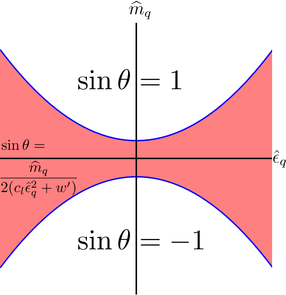
(b) First-order scenario ($w^{\prime}>0$).

Figure 4: Phase diagrams including effects of discretization and nondegeneracy for maximally $\tau_{3}$-twisted quarks. Electromagnetism has no impact on the phase diagram. Notation as in Fig. 1. The neutral pion is massless along the second-order phase boundary between shaded (CP-violating) and unshaded phases.

The resulting phase diagrams are shown in Fig. 4. Comparing to the untwisted results of Fig. 1, we see that the role of the Aoki and first-order scenarios has interchanged. Without loss of generality, we can take $n_{3}=1$ throughout the phase plane. Then, in the continuum-like (unshaded) phases we have $\sin\theta={\rm sign}(\widehat{m}_{q})$, corresponding to the condensate aligning or antialigning with the applied twist. Second order transitions occur at $|\widehat{m}_{q}|=2(w^{\prime}+c_{\ell}\widehat{\epsilon}_{q}^{2})$. For smaller values of $|\widehat{m}_{q}|$ the condensate angle is $\sin\theta=\widehat{m}_{q}/(2[w^{\prime}+c_{\ell}\widehat{\epsilon}_{q}^{2}])$, with two degenerate minima having opposite signs of $\cos\theta$. If one switches to the “physical basis” in which the twist is put on the Wilson term, then one finds that this phase violates CP, just as in the Wilson case.

These results differ significantly from the phase structure for nondegenerate quarks with a maximal $\tau_{1}$ twist, shown in Fig. 3 of Ref. Horkel and Sharpe (2014). In particular, an additional phase found for $w^{\prime}>0$ with a $\tau_{1}$ twist is absent here. We stress again that only the theory with a $\tau_{3}$ twist, i.e. that discussed here, can incorporate electromagnetism.

For the pion masses we find the following results. Within the continuum-like phases we have

$$m_{\pi^{0}}^{2}=|\widehat{m}_{q}|-2(c_{\ell}\widehat{\epsilon}_{q}^{2}+w^{\prime})\,,\ \ m_{\pi^{\pm}}^{2}=|\widehat{m}_{q}|+2c_{\rm EM}\,,$$ (29)

while within the CP-violating phase

$$m_{\pi^{0}}^{2}=2(c_{\ell}\widehat{\epsilon}_{q}^{2}+w^{\prime})\cos^{2}\theta\,,\ \ m_{\pi^{\pm}}^{2}=2(c_{\ell}\widehat{\epsilon}_{q}^{2}+w^{\prime}+c_{\rm EM})\,.$$ (30)

As expected, only the charged pion masses are affected by electromagnetism. Plots of these results along vertical slices through the phase diagram are shown in Fig. 5.

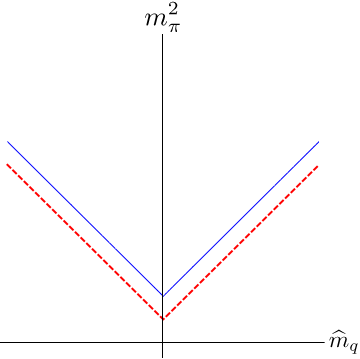
(a) Aoki scenario with $c_{\ell}\widehat{\epsilon}_{q}^{2}+w^{\prime}<-c_{\rm EM}<0$

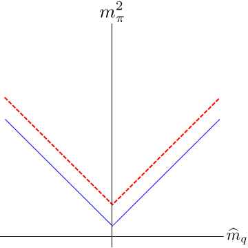
(b) Aoki scenario with $-c_{\rm EM}<c_{\ell}\widehat{\epsilon}_{q}^{2}+w^{\prime}<0$

(c) Aoki or first-order scenario with $c_{\ell}\widehat{\epsilon}_{q}^{2}+w^{\prime}>0$

Figure 5: Pion masses for nondegenerate maximally $\tau_{3}$-twisted fermions including electromagnetism. The three possible behaviors along vertical slices through phase diagrams of Fig. 4 are shown. Solid (blue) lines show $m_{\pi^{0}}^{2}$, while dashed (red) lines show $m_{\pi^{\pm}}^{2}$. Expressions for masses are given in the text.

It is interesting to compare to the results with untwisted fermions, which are given in Eqs. (8) and (9) together with the shift (16) of $m_{\pi^{\pm}}^{2}$ by $2c_{\rm EM}$ induced by electromagnetism. We see that the neutral pion mass differs only by the change of sign of $w^{\prime}$ (which also implies the interchange $\sin\theta\leftrightarrow\cos\theta$). This means that the results in the two scenarios interchange exactly. For the charged pion masses, apart from the interchange of scenarios there are also overall shifts proportional to $w^{\prime}$.

The implications of these results for present simulations are as follows. If one could simulate the theory directly (somehow dealing with the fact that the action is complex) then one would need to avoid working in or near the CP-violating phase. This is now more difficult in the first-order scenario than the Aoki scenario—opposite to the situation with untwisted Wilson fermions. This qualitative result is the same as for $\tau_{1}$ twisting (without electromagnetism), although the area taken up by unphysical phases is larger in that case Horkel and Sharpe (2014). As noted above, actual simulations done to date at maximal twist use perturbation theory in $\widehat{\epsilon}_{q}$ and $\alpha_{\rm EM}$, and so evaluate all expectation values in the theory with $\widehat{\epsilon}_{q}=\alpha_{\rm EM}=0$. Clearly, if $w^{\prime}>0$, these simulations must be careful to have $\hat{m}_{q}$ large enough to avoid the CP-violating phase.

V.2 Nonmaximal $\tau_{3}$ twist

We have also investigated the phase structure for general $\tau_{3}$ twist, i.e. nonvanishing and nonmaximal. One motivation for doing so is that twisted-mass simulations cannot achieve exactly maximal twist; another is to see how the phase diagrams of Fig. 1 change into those of Fig. 4.

Expressions are simplified if we define $\theta$ relative to a twist $\omega$, i.e. if we use

$$\langle\Sigma\rangle=e^{i\omega\tau_{3}/2}e^{i\theta\hat{n}\cdot\vec{\tau}}e^{i\omega\tau_{3}/2}\,.$$ (31)

Then we find (dropping constants)

$$-\frac{\cal V}{f^{2}} =\widehat{m}_{q}\cos\theta+c_{\ell}\widehat{\epsilon}_{q}^{2}n_{3}^{2}\sin^{2}\theta$$

$$\quad+w^{\prime}(\cos\theta\cos\omega-n_{3}\sin\theta\sin\omega)^{2}$$

$$\quad+c_{\rm EM}(\cos^{2}\theta+n_{3}^{2}\sin^{2}\theta)\,.$$ (32)

This is not amenable to simple analytic extremization, and we have used a mix of analytic and numerical methods. One can show analytically that the minima always occur at $|n_{3}|=1$. This implies that, once again, the electromagnetism does not play a role in determining the phase structure.

The sign of $n_{3}$ can always be absorbed into $\theta$, so we can again choose $n_{3}=1$ without loss of generality. The potential can then be written (up to $\theta$-independent terms) as

$$-\frac{\cal V}{f^{2}}\Bigg{|}_{n_{3}=1} =\widehat{m}_{q}\cos\theta+\cos^{2}\theta\left[-c_{\ell}\widehat{\epsilon}_{q}^{2}+w^{\prime}\cos(2\omega)\right]$$

$$\quad-\frac{w^{\prime}}{2}\sin(2\theta)\sin(2\omega)\,.$$ (33)

A numerical investigation of this potential finds that, for nonextremal $\omega$, and for all nonzero $w^{\prime}$, there is a first-order transition as $\widehat{m}_{q}$ passes through zero, irrespective of the value of $\widehat{\epsilon}_{q}$. At this transition $\theta$ jumps from $\pi/2-\delta$ to $\pi/2+\delta$, with $\delta\neq 0$ depending on the parameters. Thus, unlike at the extremal points $\omega=0,\pi/2$, there are no second-order transition lines. Correspondingly, there are no values of the parameters for which any of the pion masses vanish. This is very different from the theory with a $\tau_{1}$ twist, where we found a two-dimensional critical sheet Horkel and Sharpe (2014) in ${\widehat{m}_{q},\widehat{\epsilon}_{q},\omega}$ space.

The absence of critical lines at nonextremal twist can be understood in terms of symmetries. For $\omega=0$ and $\pi/2$, the potential has a $\theta\to-\theta$ symmetry, and this $Z_{2}$ symmetry is broken by the condensate in the CP-violating phase, leading to a massless pion at the transition. For nonextremal twist, however, the potential of Eq. (32) has no such symmetry. Lacking this symmetry, one expects, and finds, only first-order transitions.

VI Conclusions

This work completes our study of how isospin breaking impacts the phase structure of Wilson-like and twisted-mass fermions. The main results are the phase diagrams presented in Figs. 1 and 4, together with the corresponding pion masses. These results show how the combination of discretization errors and nondegeneracy can bring unphysical phases closer to (or further away) from the physical point.

The inclusion of electromagnetism into the analysis turns out to be very straightforward, aside from the need to introduce independent up and down critical masses. Electromagnetism has no impact on the phase diagrams at leading order, because the condensates in the CP-violating phases involve neutral pions. The only impact is to uniformly increase the charged pion masses.

We have investigated within W$\chi$PT the conditions used in Ref. de Divitiis et al. (2013) to determine the two critical masses in the presence of electromagnetism. We find that, unless one makes the electroquenched approximation, the two conditions are in fact not independent. To determine both critical masses one needs an additional condition, and we have presented one possibility in Appendix B. Our condition requires simulating at nonzero (though small) $\theta_{\rm QCD}$, and thus will be difficult to implement in practice, but provides an existence proof that an alternative condition exists.

Our analysis has been carried out in infinite volume. For the finite volumes used in lattice simulations one might be concerned about significant finite-volume effects on the electromagnetic contributions. The impact on the results presented here, however, should be minimal. The phase diagram will remain unaffected by electromagnetism, while the shifts in critical masses are dominated by ultraviolet momenta, themselves insensitive to the volume. The only significant effect will be on electromagnetic mass shifts, with $c_{\rm EM}$ picking up an effective power-law volume dependence Hayakawa and Uno (2008); Davoudi and Savage (2014); Borsanyi et al. (2015); Basak et al. (2014).

Appendix A Relating lattice masses to those in $\chi$PT

In this appendix we describe how bare lattice masses used in simulations with Wilson-like fermions are related to the masses $m_{u}$ and $m_{d}$ appearing in $\chi$PT (contained in the mass matrix $M$). This discussion draws heavily from the results of Ref. Bhattacharya et al. (2006). We do not consider the impact of electromagnetism here; this is discussed in the subsequent appendix.

We must assume that the number of dynamical quarks in the underlying simulations is $N_{f}=3$ (up, down and strange) or $N_{f}=4$ (adding charm). Working with up and down quarks alone turns out not to be sufficient, but in any case this is not the physical theory. We must also have that $am_{f}\ll 1$ for all flavors $f$, so that an expansion in these quantities makes sense. This condition is met by state-of-the-art simulations. Note that this condition is much weaker than the requirement that the quarks are light in the sense of $\chi$PT, which is $m_{f}\ll\Lambda_{\rm QCD}$. In the main text, we assume the latter condition holds only for up and down quarks.

Let $m_{0,f}$ be the bare dimensionless lattice mass for flavor $f$ (i.e. the mass appearing in the lattice action). Because of the additive renormalization induced by explicit chiral symmetry breaking, unrenormalized quark masses are given by

$$\widetilde{m}_{f}=\frac{m_{0,f}-m_{cr}}{a}\,,$$ (34)

where $m_{cr}$ is the (dimensionless) critical mass for the given number of dynamical flavors. Methods to determine $m_{cr}$ are described below. Then, as shown in Ref. Bhattacharya et al. (2006), renormalized masses are given by

$$m_{f}=Z_{m}\left[\widetilde{m}_{f}+(r_{m}-1)\frac{\sum_{f}\widetilde{m}_{f}}{N_{f}}+{\cal O}(a\widetilde{m}^{2})\right]\,.$$ (35)

Here $Z_{m}$ is the renormalization constant for flavor nonsinglet mass combinations such as $\epsilon_{q}=(m_{u}\!-\!m_{d})/2$, while $Z_{m}r_{m}$ is the corresponding constant for the average quark mass. $r_{m}-1$ is a finite constant, arising first at ${\cal O}(g^{4})$ in perturbation theory. By implementing continuum Ward-Takahashi identities, one can determine $r_{m}$ nonperturbatively for $N_{f}=3$ and $4$, although not for $N_{f}=2$ Bhattacharya et al. (2006). This is the reason for the restriction on $N_{f}$ noted above. We assume here that $r_{m}$ has been calculated in this way.

Equation (35) shows that the renormalized mass $m_{f}$ does not vanish when $\tilde{m}_{f}=0$ if other flavors are massive. Specifically, for the up and down quarks we have

$$m_{u}+m_{d} =Z_{m}\frac{1\!+\!r_{m}}{2}(\widetilde{m}_{u}+\widetilde{m}_{d})$$

$$\ \ +Z_{m}\frac{r_{m}\!-\!1}{2}(\widetilde{m}_{s}+\widetilde{m}_{ch})\,,$$ (36)

$$m_{u}-m_{d} =Z_{m}(\tilde{m}_{u}-\tilde{m}_{d})\,.$$ (37)

(Here we we have chosen $N_{f}=4$ for definiteness; the result for $N_{f}=3$ is similar.) Thus the two-flavor massless point receives an overall additive shift due to the strange and charm quarks, and we also see explicitly the difference between singlet and nonsinglet renormalizations.

These results imply that, in terms of unrenormalized masses, the phase diagrams of Fig. 1 would be translated in the vertical direction (due to the additive mass shift) and stretched by different factors in the vertical and horizontal directions. The respective stretch factors are $B_{0}Z_{m}(1+r_{m})/2$ and $B_{0}Z_{m}$. If, however, $r_{m}$ is known, then the two stretch factors can be made equal by applying a finite renormalization to remove the $(1+r_{m})/2$ factor. Knowledge of $Z_{m}$ is, however, not useful, since it always appears multiplied by the unknown LEC $B_{0}$.

We would like to be able to remove the additive mass shift in Eq. (36). To do so we consider how the critical mass $m_{cr}$ is determined. The expressions above assume that it has been obtained by doing simulations with $N_{f}$ degenerate quarks of mass $m$, and equating $m_{cr}$ to the value of $m$ at which the “PCAC mass” vanishes. This is equivalent to imposing

$$\langle\pi^{+}|\partial_{\mu}(\bar{u}\gamma_{\mu}\gamma_{5}d)|0\rangle\Big{|}_{m=m_{cr}}=0\,.$$ (38)

If, instead, one imposes this condition by varying $m=m_{u}=m_{d}$, with $m_{s}$ and $m_{ch}$ held fixed at their physical values, then the $m_{cr}$ so obtained automatically includes the shift due to loops of strange and charm quarks. This is because one is enforcing a consequence of chiral symmetry in the two-flavor subsector. With this new choice of $m_{cr}$, and with the adjustment of stretch factors described above, the phase diagrams of Fig. 1 apply directly for lattice masses $\tilde{m}_{f}$.

This new choice of $m_{cr}$ has a second advantage: it removes an additional shift of $O(a)$ in the relation between bare quark masses and the masses appearing in $\chi$PT. As explained in Ref. Sharpe and Singleton (1998), this shift is caused by the ${\cal O}(a)$ clover term in the Symanzik effective action (and is thus absent for nonperturbatively improved Wilson fermions). In the main text it is assumed that this shift has been removed.

Since we include ${\cal O}(a^{2})$ terms in the main text, we must determine how they impact the considerations above. There is no further shift in the quark masses at this order—this next occurs at ${\cal O}(a^{3})$ Sharpe (2005). However, as illustrated by Fig. 1, the ${\cal O}(a^{2})$ terms do impact the phase diagram. This means that, in general, one cannot use the vanishing of the PCAC mass to determine $m_{cr}$ with untwisted Wilson fermions. For example, if one is in the first-order scenario [Fig. 1(b) along the $\hat{m}_{q}$ axis], then the PCAC mass simply does not vanish for any $\hat{m}_{q}$. Instead, one must introduce a twisted component to the mass, $\mu\sim{\cal O}(a)$, and then enforce the vanishing of the PCAC mass (in the so-called “twisted basis”). Extrapolating the result linearly to $\mu=0$ yields a result for $m_{cr}$ that has errors of ${\cal O}(a^{3})$, which is sufficiently accurate for our analysis. For a detailed discussion of this point see Ref. Sharpe (2005).

In summary, by determining $r_{m}$ from Ward identities, and the critical mass from the PCAC mass condition with twisted-mass quarks, one can obtain lattice quark masses which are proportional to those appearing in $\chi$PT at the order we work. Specifically, we find

$$\frac{\widehat{m}_{q}}{B_{0}Z_{m}}=\frac{1\!+\!r_{m}}{2}(\tilde{m}_{u}\!+\!\tilde{m}_{d})\ {\rm and}\ \ \frac{\widehat{\epsilon}_{q}}{B_{0}Z_{m}}=(\tilde{m}_{u}\!-\!\tilde{m}_{d})\,,$$ (39)

where $\widehat{m}_{q}$ and $\widehat{\epsilon}_{q}$ are the quantities appearing in the chiral potential of Eq. (5).

This analysis can be straightforwardly extended to arbitrary twist. We begin with maximal twist, for which the mass matrix in $\chi$PT is given by Eq. (27), and the relevant bare masses are $\mu_{0}$ and $\eta_{0}$ of Eq. (23). In this case there is no additive renormalization, but the presence of different renormalization factors for singlet and nonsinglet masses remains. Using the results of Ref. Bhattacharya et al. (2006), we find

$$\frac{\widehat{m}_{q}}{B_{0}Z_{m}}=\frac{Z_{S}}{Z_{P}}\frac{1\!+\!r_{P}}{r_{P}}\mu_{0}\ \ {\rm and}\ \ \frac{\widehat{\epsilon}_{q}}{B_{0}Z_{m}}=\frac{Z_{S}}{Z_{P}}\eta_{0}\,.$$ (40)

Here $Z_{S}/Z_{P}$ and $r_{P}$ are finite constants, both of which can be determined from Ward identities for $N_{f}=3$ and $4$, but not for $N_{f}=2$ Bhattacharya et al. (2006). Like $r_{m}$, $r_{P}$ begins at ${\cal O}(g^{4})$ in perturbation theory.

At arbitrary twist one has four bare masses, and they are related to the corresponding four renormalized masses using the same renormalization factors as given in Eqs. (39) and (40).

Finally, we stress that the analysis presented here does not include electromagnetic effects. The dominant such effect is that the critical mass $m_{cr}$ has to be chosen differently for the up and down quarks, and is discussed in the following appendix. A subdominant, but still important, effect is that the renormalization factors now depend not only on $\alpha_{S}$ but also on $\alpha_{\rm EM}$. The latter dependence can presumably be adequately captured using perturbation theory. The formulae given above still hold if one uses the new critical masses and renormalization factors.

Appendix B Determining the critical masses in the presence of electromagnetism

The analysis of the previous appendix must be extended when electromagnetism is included, due to the presence of charge-dependent self energy corrections proportional to $\alpha_{\rm EM}/a$. This implies that the critical masses for up and down quarks differ, and we label them $m_{cr,u}$ and $m_{cr,d}$, respectively. In Ref. de Divitiis et al. (2013) two methods for a nonperturbative determination of these critical masses are proposed. One of these (the method used in practice in Ref. de Divitiis et al. (2013)) involves only up and down quarks, and thus can be implemented, and therefore checked, within SU(2) W$\chi$PT. We do so in this appendix, finding that the method does not fix both critical masses, but rather constrains them to lie in a one-dimensional subspace of the $m_{cr,u}$—$m_{cr,d}$ plane. We then provide an additional condition that does completely determine $m_{cr,u}$ and $m_{cr,d}$.

The tuning conditions require the use of twisted-mass quarks, although the resulting values of $m_{cr,u}$ and $m_{cr,d}$ apply for both Wilson and twisted-mass quarks. Thus the lattice quark Lagrangian is given by Eq. (23). We can write the mass matrix in two useful forms

$$m_{0}+\tau_{3}\epsilon_{0}+i\gamma_{5}\tau_{3}\mu_{0}+i\gamma_{5}\eta_{0}\\ =\begin{pmatrix}m_{0,u}+i\gamma_{5}\mu_{0,u}&0\\ 0&m_{0,d}-i\gamma_{5}\mu_{0,d}\\ \end{pmatrix}\,.$$ (41)

The tuning proceeds by first choosing bare twisted masses $\mu_{0,u}$ and $\mu_{0,d}$ such that, when multiplicatively renormalized as described in the previous appendix, they give rise, respectively, to the desired physical up and down quark masses. The negative sign multiplying $\mu_{0,d}$ is chosen to correspond to a $\tau_{3}$ twist. The second step is to tune the untwisted masses $m_{0,u}$ and $m_{0,d}$ to their critical values such that the (additively) renormalized untwisted masses vanish.

The method of determining $m_{cr}$ used in the previous section is no longer useful—the vanishing of the PCAC mass is a condition based on the recovery of the chiral SU(2) group, but this group is explicitly broken by electromagnetism. The workaround proposed in Ref. de Divitiis et al. (2013) is to add to the sea quarks (labeled $u_{S}$ and $d_{S}$) a pair of valence quarks, $u_{V}$ and $d_{V}$, each of which has the same charge and untwisted mass as the corresponding sea quark, but has opposite twisted mass. Thus $(u_{S},u_{V})$ and $(d_{V},d_{S})$ each form a twisted pair. The key point is that, within each pair, the ${\cal O}(\alpha_{\rm EM}/a)$ shift in the untwisted mass is common. Therefore it is plausible that one can determine the critical mass for each pair by enforcing the recovery of the corresponding valence-sea chiral SU(2). Specifically, $m_{cr,u}$ is determined by

$$\langle\pi^{u}_{SV}|\partial_{\mu}(\bar{u}_{S}\gamma_{\mu}\gamma_{5}u_{V})|0\rangle\Big{|}_{m_{0,u}=m_{cr,u}}=0\,,$$ (42)

while $m_{cr,d}$ is determined by the analogous condition with $u\to d$:

$$\langle\pi^{d}_{SV}|\partial_{\mu}(\bar{d}_{S}\gamma_{\mu}\gamma_{5}d_{V})|0\rangle\Big{|}_{m_{0,d}=m_{cr,d}}=0\,.$$ (43)

Here $\pi^{u}_{SV}$ and $\pi^{d}_{SV}$ are sea-valence pions composed, respectively, of up and down quarks.

When using a partially quenched theory, one also needs to add ghost fields, $\tilde{u}_{V}$ and $\tilde{d}_{V}$, to cancel the valence quark determinants. Thus the full softly-broken chiral symmetry is the graded group $SU(4|2)_{L}\times SU(4|2)_{R}$. This raises the question of whether complications arising from partial quenching, or from discretization effects, can lead to corrections to the tuning criteria of Eqs. (42) and (43). This is one of the issues we address here by mapping these conditions into $\chi$PT.

We begin by mapping the mass matrix in the unquenched sector into $\chi$PT. The four parameters of Eq. (41) map into

$$\chi =\begin{pmatrix}\hat{m}_{u}e^{i\omega_{u}}&0\\ 0&\hat{m}_{d}e^{-i\omega_{d}}\\ \end{pmatrix}$$ (44)

$$=\begin{pmatrix}(\widehat{m}_{q}+\widehat{\epsilon}_{q})e^{i(\omega+\varphi)}&0\\ 0&(\widehat{m}_{q}-\widehat{\epsilon}_{q})e^{i(-\omega+\varphi)}\\ \end{pmatrix}\,.$$ (45)

The choice of sign for $\omega_{d}$ is such that it is positive with a $\tau_{3}$ twist. $\chi$ contains the additional parameter $\varphi$ compared to the mass matrix analyzed in the main text, Eq. (26). $\varphi$ is a measure of the difference between up and down twist angles,

$$\omega_{u}=\omega+\varphi\,,\qquad\omega_{d}=\omega-\varphi\,.$$ (46)

As discussed in Sec. V, such a difference corresponds to the introduction of a nonzero $\theta_{\rm QCD}$—the explicit relation is $\varphi=\theta_{\rm QCD}/2$.

We note that the relations between the bare masses of Eq. (41) and the parameters of $\chi$ in Eq. (45)—which can be worked out along the lines of the previous appendix—are not needed here. All we need to know is that, if $m_{0,u}=m_{cr,u}$ and $m_{0,d}=m_{cr,d}$, then both up and down masses are fully twisted. Thus the twist angles in $\chi$ are $\omega_{u}=\omega_{d}=\pi/2$, implying maximal twist with no $\theta_{\rm QCD}$ term: $\omega=\pi/2$ and $\varphi=0$. Reaching this point in parameter space is the aim of tuning.

When considering the PQ extension of this theory, we will focus mainly on the quark sector, since the ghosts do not play a significant role. Collecting the four quark fields in the order

$$\psi_{{PQ}}^{\top}=(u_{S},u_{V},d_{V},d_{S})\,,$$ (47)

the extended quark mass matrix is

$$\chi_{{PQ}}=\begin{pmatrix}(\widehat{m}_{q}+\widehat{\epsilon}_{q})e^{i\omega_{u}\tau_{3}}&0\\ 0&(\widehat{m}_{q}-\widehat{\epsilon}_{q})e^{i\omega_{d}\tau_{3}}\\ \end{pmatrix}\,.$$ (48)

The factors of $\tau_{3}$ arise because, by construction, valence quarks have opposite twisted masses to the corresponding sea quarks. We stress that the ${\cal O}(\alpha_{\rm EM}/a)$ shifts are incorporated into the parameters $\widehat{m}_{q}$ and $\widehat{\epsilon}_{q}$, along with the usual ${\cal O}(1/a)$ shifts. We can also include the ${\cal O}(a)$ shifts in the same fashion.

To implement the conditions (42) and (43) in the PQ theory, we need the extension of $\Sigma$ to this theory. This is a $6\times 6$ matrix transforming in the usual way under $SU(4|2)_{L}\times SU(4|2)_{R}$. In fact, as we only need matrix elements for states composed of quarks, and since we know from Ref. Bar et al. (2011) that there are no quark-ghost condensates, we can focus on the $4\times 4$ quark sub-block, which we call $\Sigma_{{PQ}}$. We now argue that the expectation value of $\Sigma_{{PQ}}$ has the form

$$\langle\Sigma_{{PQ}}\rangle={\rm diag}(e^{i\theta},e^{-i\theta},e^{i\theta},e^{-i\theta})\,.$$ (49)

This is based on the following results. First, the unquenched $2\times 2$ block of $\Sigma_{{PQ}}$ (i.e. that involving the first and last rows and columns) is just the unquenched $\Sigma$ field. This is unaffected by partial quenching Sharpe and Shoresh (2000, 2001), and its expectation value is given by an unquenched $\chi$PT calculation. This calculation must include not only nondegeneracy, electromagnetism and twist, but also nonvanishing $\theta_{\rm QCD}$. To our knowledge such an analysis has not previously been done, so we carry it out in a companion paper Horkel and Sharpe (2015). The result is that the unquenched condensate $\langle\Sigma\rangle$ only rotates in the $\tau_{3}$ direction—there are no off-diagonal condensates such as $\langle\bar{u}_{S}d_{S}\rangle$. This fixes the first and last entries in Eq. (49) to have opposite phase angles.

This is an important result for the following, so we emphasize its key features. Although $\theta_{\rm QCD}\neq 0$ leads to an overall phase in the mass matrix [$e^{i\varphi}$ in Eq. (45)], its effect on the condensate $\langle\Sigma\rangle$ is qualitatively similar to that of a twist $\omega$, despite the fact that the latter leads to opposite phases on $u$ and $d$ quarks. This happens because $\Sigma$ is constrained to lie in $SU(2)$, and so has no way to break parity other than rotating in the $\tau_{3}$ direction. An overall phase rotation would take it out of $SU(2)$ into the $U(2)$ manifold.

The second result needed to obtain Eq. (49) is the existence of relations between valence and sea-quark condensates. In particular, one can show that

$$\langle\bar{u}_{V}u_{V}\rangle=\langle\bar{u}_{S}u_{S}\rangle\ \ {\rm and}\ \ \langle\bar{u}_{V}\gamma_{5}u_{V}\rangle=-\langle\bar{u}_{S}\gamma_{5}u_{S}\rangle\,,$$ (50)

to all orders in the hopping parameter expansion. The minus sign in the second relation follows from the opposite twisted mass of sea and valence quarks. The result (50) holds on each configuration and thus also for the ensemble average, even though the measure is complex for $\theta_{\rm QCD}\neq 0$. Since the additive and multiplicative renormalizations of these condensates are the same for valence and sea quarks, the result (50) implies that valence and sea up-quark condensates have opposite “twists”, $e^{\pm i\theta}$. The same argument applies to the down-quark condensates, and taken together these arguments determine the form of the second and third diagonal elements in Eq. (49).

The final result needed to obtain the form (49) is the vanishing of off-diagonal condensates involving one or more valence quarks, e.g. $\langle\bar{u}_{V}d_{V}\rangle$ and $\langle\bar{u}_{V}d_{S}\rangle$. These differ from the diagonal condensates in that there is no mass term in the quark-level Lagrangian that can serve as a source for such condensates. Thus to determine whether they are nonzero one must add a source, e.g. $\Delta\,\bar{d}_{V}u_{V}$, calculate the resulting condensate, send the volume to infinity, and finally send the parameter $\Delta\to 0$. This analysis has been carried out in Appendix A of Ref. Hansen and Sharpe (2012) in a theory with twisted-mass quarks, although, unlike our situation, the quarks were degenerate and $\theta_{\rm QCD}=0$. The general lessons from Ref. Hansen and Sharpe (2012) are (i) that to obtain a nonvanishing condensate one needs a source of infrared divergence to cancel the overall factor of $\Delta$, and (ii) that nonvanishing twisted masses cut off such divergences. These lessons apply also for all the off-diagonal condensates that we consider here. However, the argument as given in Ref. Hansen and Sharpe (2012) assumes that the measure is real and positive, which does not hold here. Nevertheless, since we are tuning to $\theta_{\rm QCD}=0$, we expect the impact of having a complex measure to be small. Furthermore, we know from Ref. Horkel and Sharpe (2015) that the corresponding sea quark condensates, e.g. $\langle\bar{u}_{S}d_{S}\rangle$ and $\langle\bar{u}_{S}\gamma_{5}d_{S}\rangle$, vanish even when $\theta_{\rm QCD}\neq 0$. These condensates differ from those containing valence quarks only by changing the signs of some of the twisted masses. Since it is the presence of these masses, and not their detailed properties, that leads to the vanishing of the condensate, we expect the result holds for all off-diagonal condensates.

With the form (49) in hand, we can now apply the tuning conditions (42) and (43) in $\chi$PT. We do so by generalizing the analysis of Ref. Sharpe and Wu (2005), where the twist angle for unquenched twisted-mass fermions was determined in $\chi$PT by applying a PCAC-like condition. The required extension is from the $SU(2)$ sea-quark sector alone to the full valence-sea $SU(4)$ symmetry. Much of the analysis carries over with minimal changes from Ref. Sharpe and Wu (2005), so we only sketch the calculation.

The first step is to obtain the pion fields that couple to external particles in the tuning conditions. Following Ref. Sharpe and Wu (2005), we obtain these by expanding the chiral field about its vacuum value as

$$\Sigma_{{PQ}} =\xi_{PQ}\,e^{2i\Pi/f}\,\xi_{PQ}\,,$$ (51)

$$\Pi =\sum_{a=1}^{15}\pi_{a}\lambda_{a}\,,$$ (52)

$$\xi_{PQ} =\sqrt{\langle\Sigma_{{PQ}}\rangle}={\rm diag}(e^{i\theta/2},e^{-i\theta/2},e^{i\theta/2},e^{-i\theta/2})\,.$$ (53)

Here $\lambda_{a}$ are the generators of SU(4), with $\pi_{a}$ the corresponding pion fields. These are the pions in the PQ theory that are composed of quarks alone, with no ghost component. The pions needed for tuning, $\pi^{u}_{SV}$ and $\pi^{d}_{SV}$, are contained in the upper and lower diagonal $2\times 2$ blocks of $\Pi$, respectively.

The next step is to determine the form, in $\chi$PT, of the axial currents appearing in the tuning conditions. These can be obtained by introducing sources into derivatives using standard methodology. Since, by definition, our chiral potential does not contain derivatives, at LO⁺ only the LO kinetic term [shown in Eq. (2)] enters into the determination of the currents. We do not display the form of the currents, however, as the calculation needed for each of the tuning conditions is exactly the same as that carried out in Ref. Sharpe and Wu (2005). This is because each tuning condition involves a separate, nonoverlapping $SU(2)$ subgroup of $SU(4)$ (upper-left or lower-right $2\times 2$ block), and because the condensate (49) does not connect these subgroups. We simply quote the results of the calculation:

$$\langle\pi^{u}_{SV}|\partial_{\mu}(\bar{u}_{S}\gamma_{\mu}\gamma_{5}u_{V})|0\rangle \propto\cos\theta\,,$$ (54)

$$\langle\pi^{d}_{SV}|\partial_{\mu}(\bar{d}_{S}\gamma_{\mu}\gamma_{5}d_{V})|0\rangle \propto\cos\theta\,.$$ (55)

Thus enforcing either (42) or (43) has the effect of setting $\theta=\pm\pi/2$ and the condensate to

$$\langle\Sigma_{PQ}\rangle=\pm{\rm diag}(i,-i,i,-i)\,,$$ (56)

For our choices of signs of the twisted masses $\mu_{0,u}$ and $\mu_{0,d}$ in Eq. (41), the $\pm$ signs are in fact plusses, i.e. $\theta=\pi/2$.

A surprising aspect of this result is that the two tuning conditions are not independent: if one enforces, say, Eq. (42) then Eq. (43) will be automatically satisfied. This dependence arises because changing $m_{u}$ in turn changes $\varphi$ and $\omega$ and this impacts the $d$ condensate through the quark determinant. One might, therefore, wonder how the two tuning conditions have been successfully applied in Ref. de Divitiis et al. (2013). To understand this, we note that this work makes two approximations. First, isospin-breaking effects are evaluated only through linear order in an expansion in $m_{u}\!-\!m_{d}$ and $\alpha_{\rm EM}$. Second, insertions of $m_{u}\!-\!m_{d}$ or photons on sea-quark loops are dropped (the “electroquenched approximation”). The latter approximation has the effect of disconnecting the two tuning conditions—all quark loops in both conditions are evaluated with uncharged, degenerate sea-quarks, so the $u$-quark condensate cannot be impacted by changes in $m_{d}$ and vice versa. Since $\chi$PT predicts that there is a tight correlation between the condensates, it appears to us that the electroquenched approximation is theoretically problematic. However, from a purely numerical viewpoint, the dropped contributions may well lead only to small corrections.

The lack of independence implies that the tuning conditions cannot determine both $m_{u,c}$ and $m_{d,c}$—only one constraint on these two critical masses is obtained. In terms of the parameters of mass matrix (45), the conditions determine only a relation between $\omega$ and $\varphi$. Thus, after enforcing either (42) or (43) the theory is known to lie along a line in the $\omega$—$\varphi$ plane. In terms of the bare masses, the theory lies along a line in the $m_{0,u}$—$m_{0,d}$ plane (with, recall, $\mu_{0,u}$ and $\mu_{0,d}$ fixed at the values leading to physical quark masses when $m_{0,u}=m_{0,d}=0$). We do know that this one-dimensional subspace includes the point we are trying to tune to, namely that with $(\omega,\varphi)=(\pi/2,0)$. This follows from the analysis of Sec. V.1. At maximal twist with $\varphi=0$, the twist in the condensate is also maximal, i.e. $\theta=\pi/2$. The only caveat is that the values of the twisted masses must be such that one lies in the continuum-like phase, rather than the CP-violating phase (see Fig. 4).

To complete the tuning we need an additional condition that forces us to the desired point along the allowed line. At first blush one might expect that it would be simple to find an additional tuning condition, since theories with $\theta_{\rm QCD}\neq 0$ have explicit parity violation. This is in contrast to the parity violation induced by a nonzero twist $\omega$ which, in the continuum limit, can be removed by a chiral rotation. This suggests that one should look for quantities that vanish when parity is a good symmetry. The flaw in this approach is that parity is broken by $\omega\neq 0$ away from the continuum limit—the chiral rotation required to obtain the parity-symmetric form is not a symmetry on the lattice. Thus the distinction between $\varphi\neq 0$ and $\omega\neq 0$ no longer holds.

The only choice that we have found for a second condition involves using the pion masses. Specifically, we find that, along the line picked out by setting $\theta=\pi/2$, the masses of both charged and neutral pions are minimized when $\varphi=0$. This assumes only that we are in the continuum-like phase for the physical values of $\mu_{0,u}$ and $\mu_{0,d}$.

The details of the calculation are presented in Ref. Horkel and Sharpe (2015). Working at LO⁺, we find that the constraint $\theta=\pi/2$ forces the quark masses to lie on the line

$$\frac{\hat{m}_{d}}{\hat{m}_{u}}=-\left(\frac{1-c_{\ell}(\hat{\mu}_{u}-\hat{\mu}_{d})}{1+c_{\ell}(\hat{\mu}_{u}-\hat{\mu}_{d})}\right)\,.$$ (57)

As noted above, this line passes through the desired point $m_{u}=m_{d}=0$. The slope is $-1$ when $c_{\ell}=0$, and increases in magnitude as $c_{\ell}$ increases (assuming the physical situation $\hat{\mu}_{u}<\hat{\mu}_{d}$). There is no singularity when the slope reaches infinity—this simply means that the constraint line is the $m_{u}=0$ axis. For larger $c_{\ell}$ the slope is positive. It decreases with increasing $c_{\ell}$, though it always remains greater than unity. The pion masses along the constraint line are

$$m_{\pi^{0}}^{2} =\frac{\hat{\mu}_{u}\!+\!\hat{\mu}_{d}}{2}-2c_{\ell}\left(\frac{\hat{\mu}_{u}\!-\!\hat{\mu}_{d}}{2}\right)^{2}$$

$$\qquad\ \ +2c_{\ell}\left(\frac{\hat{m}_{u}\!-\!\hat{m}_{d}}{2}\right)^{2}-2w^{\prime}\,,$$ (58)

$$m_{\pi^{\pm}}^{2} =\frac{\hat{\mu}_{u}\!+\!\hat{\mu}_{d}}{2}+2c_{\ell}\left(\frac{\hat{m}_{u}\!-\!\hat{m}_{d}}{2}\right)^{2}+2c_{\rm EM}\,.$$ (59)

Thus we see that both masses are minimized along the constraint line when $m_{u}=m_{d}=0$. If one were to implement this tuning condition in practice, then one would apply it for the charged pion masses, since these have no quark-disconnected contractions.

This analysis breaks down when $c_{\ell}$ gets too large, because the theory with $m_{u}=m_{d}=0$ then lies in the the CP-violating phase. This can be seen from the result (58)—for large enough $c_{\ell}$ the squared neutral pion mass becomes negative. This happens sooner for the first-order scenario, $w^{\prime}>0$.

We close this section by commenting on the impact of higher-order terms in $\chi$PT. Because of such terms, even if one perfectly implements our two tuning conditions—namely either Eq. (42) or (43) and minimizing the pion masses—one will not have precisely tuned to $m_{u}=m_{d}=0$. This can be seen, for example, from the analysis of Ref. Sharpe and Wu (2005), where terms of ${\cal O}(ap^{2},am)$ lead to maximal twist occurring at untwisted masses of ${\cal O}(a\mu)$, with $\mu$ the twisted mass, rather than zero. Shifts of this size occur also in the presence of isospin breaking, although the detailed form of the corrections will differ. Within our power-counting, however, $\mu\sim a^{2}$ so that the shifts in the untwisted masses are $\sim{\cal O}(a^{3})$, beyond the order that we consider.

References

- Aoki (1984) S. Aoki, Phys.Rev. D30, 2653 (1984).
- Sharpe and Singleton (1998) S. R. Sharpe and J. Singleton, Robert L., Phys.Rev. D58, 074501 (1998), arXiv:hep-lat/9804028 [hep-lat] .
- Horkel and Sharpe (2014) D. P. Horkel and S. R. Sharpe, Phys.Rev. D90, 094508 (2014), arXiv:1409.2548 [hep-lat] .
- Portelli (2013) A. Portelli, PoS KAON13, 023 (2013), arXiv:1307.6056 [hep-lat] .
- Tantalo (2014) N. Tantalo, PoS LATTICE2013, 007 (2014), arXiv:1311.2797 [hep-lat] .
- Dashen (1971) R. F. Dashen, Phys.Rev. D3, 1879 (1971).
- Creutz (2004) M. Creutz, Phys.Rev.Lett. 92, 201601 (2004), arXiv:hep-lat/0312018 [hep-lat] .
- Borsanyi et al. (2015) S. Borsanyi, S. Durr, Z. Fodor, C. Hoelbling, S. Katz, et al., Science 347, 1452 (2015), arXiv:1406.4088 [hep-lat] .
- Frezzotti and Rossi (2004) R. Frezzotti and G. Rossi, Nucl.Phys.Proc.Suppl. 128, 193 (2004), arXiv:hep-lat/0311008 [hep-lat] .
- Carrasco et al. (2014) N. Carrasco et al. (European Twisted Mass), Nucl. Phys. B887, 19 (2014), arXiv:1403.4504 [hep-lat] .
- de Divitiis et al. (2013) G. de Divitiis et al. (RM123 Collaboration), Phys.Rev. D87, 114505 (2013), arXiv:1303.4896 [hep-lat] .
- de Divitiis et al. (2012) G. de Divitiis, P. Dimopoulos, R. Frezzotti, V. Lubicz, G. Martinelli, et al., JHEP 1204, 124 (2012), arXiv:1110.6294 [hep-lat] .
- Horkel and Sharpe (2015) D. P. Horkel and S. R. Sharpe, (2015), arXiv:1507.03653 [hep-lat] .
- Aoki et al. (2014) S. Aoki et al., Eur. Phys. J. C74, 2890 (2014), arXiv:1310.8555 [hep-lat] .
- Olive et al. (2014) K. Olive et al. (Particle Data Group), Chin.Phys. C38, 090001 (2014).
- Gasser and Leutwyler (1985) J. Gasser and H. Leutwyler, Nucl.Phys. B250, 465 (1985).
- Hayakawa and Uno (2008) M. Hayakawa and S. Uno, Prog.Theor.Phys. 120, 413 (2008), arXiv:0804.2044 [hep-ph] .
- Davoudi and Savage (2014) Z. Davoudi and M. J. Savage, Phys.Rev. D90, 054503 (2014), arXiv:1402.6741 [hep-lat] .
- Portelli et al. (2010) A. Portelli et al. (Budapest-Marseille-Wuppertal Collaboration), PoS LATTICE2010, 121 (2010), arXiv:1011.4189 [hep-lat] .
- Symanzik (1983a) K. Symanzik, Nucl.Phys. B226, 187 (1983a).
- Symanzik (1983b) K. Symanzik, Nucl.Phys. B226, 205 (1983b).
- Gupta et al. (1984) R. Gupta, G. Kilcup, and S. R. Sharpe, Phys.Lett. B147, 339 (1984).
- Ecker et al. (1989) G. Ecker, J. Gasser, A. Pich, and E. de Rafael, Nucl.Phys. B321, 311 (1989).
- Witten (1983) E. Witten, Phys.Rev.Lett. 51, 2351 (1983).
- Golterman and Shamir (2014) M. Golterman and Y. Shamir, Phys.Rev. D89, 054501 (2014), arXiv:1401.0356 [hep-lat] .
- Baron et al. (2011) R. Baron et al. (European Twisted Mass Collaboration), Comput.Phys.Commun. 182, 299 (2011), arXiv:1005.2042 [hep-lat] .
- Frezzotti et al. (2001) R. Frezzotti, P. A. Grassi, S. Sint, and P. Weisz (Alpha collaboration), JHEP 0108, 058 (2001), arXiv:hep-lat/0101001 [hep-lat] .
- Walker-Loud and Wu (2005) A. Walker-Loud and J. M. Wu, Phys.Rev. D72, 014506 (2005), arXiv:hep-lat/0504001 [hep-lat] .
- Munster (2004) G. Munster, JHEP 0409, 035 (2004), arXiv:hep-lat/0407006 [hep-lat] .
- Scorzato (2004) L. Scorzato, Eur.Phys.J. C37, 445 (2004), arXiv:hep-lat/0407023 [hep-lat] .
- Sharpe and Wu (2004) S. R. Sharpe and J. M. Wu, Phys.Rev. D70, 094029 (2004), arXiv:hep-lat/0407025 [hep-lat] .
- Basak et al. (2014) S. Basak et al. (MILC), PoS LATTICE2014, 116 (2014), arXiv:1409.7139 [hep-lat] .
- Bhattacharya et al. (2006) T. Bhattacharya, R. Gupta, W. Lee, S. R. Sharpe, and J. M. Wu, Phys.Rev. D73, 034504 (2006), arXiv:hep-lat/0511014 [hep-lat] .
- Sharpe (2005) S. R. Sharpe, Phys.Rev. D72, 074510 (2005), arXiv:hep-lat/0509009 [hep-lat] .
- Sharpe (2006) S. Sharpe, (2006), arXiv:hep-lat/0607016 [hep-lat] .
- Golterman (2009) M. Golterman, (2009), arXiv:0912.4042 [hep-lat] .
- Bar et al. (2011) O. Bar, M. Golterman, and Y. Shamir, Phys.Rev. D83, 054501 (2011), arXiv:1012.0987 [hep-lat] .
- Sharpe and Shoresh (2000) S. R. Sharpe and N. Shoresh, Phys.Rev. D62, 094503 (2000), arXiv:hep-lat/0006017 [hep-lat] .
- Sharpe and Shoresh (2001) S. R. Sharpe and N. Shoresh, Phys.Rev. D64, 114510 (2001), arXiv:hep-lat/0108003 [hep-lat] .
- Hansen and Sharpe (2012) M. T. Hansen and S. R. Sharpe, Phys.Rev. D85, 014503 (2012), arXiv:1111.2404 [hep-lat] .
- Sharpe and Wu (2005) S. R. Sharpe and J. M. Wu, Phys.Rev. D71, 074501 (2005), arXiv:hep-lat/0411021 [hep-lat] .