Direct Measurement of the Surface Tension of Nanobubbles

Abstract

It is shown that when the nanobubble contact line is pinned to a penetrating tip the interface behaves like a Hookean spring with spring constant proportional to the nanobubble surface tension. Atomic force microscope (AFM) data for several nanobubbles and solutions are analysed and yield surface tensions in the range 0.04–0.05 N/m (compared to 0.072 N/m for saturated water), and supersaturation ratios in the range 2–5. These are the first direct measurements of the surface tension of a supersaturated air-water interface. The results are consistent with recent theories of nanobubble size and stability, and with computer simulations of the surface tension of a supersaturated solution.

I Introduction

Experimental evidence for nanobubbles was first published in 1994, Parker94 and since then their existence has been confirmed from various features of the measured forces between hydrophobic surfaces, Carambassis98 ; Tyrrell01 ; Tyrrell02 including a reduced attraction in de-aerated water, Wood95 ; Meagher94 ; Considine99 ; Mahnke99 ; Ishida00 ; Meyer05 ; Stevens05 and from images obtained with tapping mode atomic force microscopy. Tyrrell01 ; Tyrrell02 ; Ishida00 ; Holmberg03 ; Simonsen04 ; Zhang04 ; Zhang06a ; Zhang06b ; Yang07 For a recent review of theory and experiment, see Ref. Attard14, .

The initial controversies over the existence of nanobubbles —that they should have an internal gas pressure of 10–100 atmospheres that would cause them to dissolve in microseconds— have largely been resolved. First it was shown that nanobubbles can only be in equilibrium in water supersaturated with air,Moody02 and then it was shown that the surface tension of a supersaturated solution must be less than that of a saturated solution.Moody03 Finally, it was shown that nanobubbles with a pinned contact rim are thermodynamically stable.Attard15 This means that contact line pinning is a necessary and sufficient condition for nanobubbles to be in mechanical and diffusive equilibrium with the supersaturated solution.

The significance of the reduction in surface tension is that the internal gas pressure, which can be calculated from the Laplace-Young equation, is much less than those initial estimates used to argue against nanobubbles. It also means that the degree of supersaturation of the solution, necessary for diffusive equilibrium of the nanobubble, is reduced to realistic levels that are attainable in the fluid cell.

For many it is surprising that purely on thermodynamic grounds (ie. no additives or surfactant) the surface tension for nanobubbles should be reduced from the usual value of the air-water interface. Nevertheless, this result is firmly established by thermodynamics,Moody03 density functional theory,Cahn59 ; Oxtoby88 ; Oxtoby98 and computer simulation.Thompson84 ; Moody04 ; He05 The result is not widely acknowledged within the nanobubble field, possibly because many practitioners place more trust in experimental measurement than they do in thermodynamics or in mathematical equations. To close this gap, it would be desirable to measure directly the surface tension of nanobubbles.

Measuring the surface tension of the supersaturated air-water interface is a worthwhile experimental goal that has application beyond nanobubbles. For example, in atmospheric physics the nucleation of cloud droplets always occurs from a supersaturated atmosphere, and so the rate of change of surface tension with the degree of supersaturation is a key input necessary for quantitative modeling in that field.

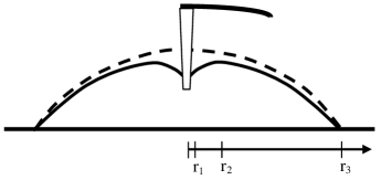
Figure 1: Hemispherical bubble penetrated and deformed by a conical tip (blunt radius $r_{0}$, height $z_{0}$) upon which it sticks at $r_{1}$.

A supersaturated solution in the current context means that the concentration of air in the water is higher than it would be if the water were equilibrated with air at the current temperature and pressure. Supersaturation can be readily achieved by previously equilibrating the water with air at a higher pressure or at a lower temperature. The difficulty in measuring directly the surface tension of a supersaturated solution is that the change in surface tension is determined by the concentration of air within the first nanometer of the interface, but, due to diffusion across the interface, this region is always saturated rather than supersaturated, at least if the measurement is performed on a macroscopic droplet or bubble exposed to the atmosphere. In the case of nanobubbles, however, the solution is supersaturated immediately in the vicinity of the interface due to the high internal gas pressure of the nanobubble, and so the surface tension of a nanobubble must be that of a supersaturated solution. If one could measure the surface tension of the nanobubble, then one would have a means to determine the rate of change of surface tension with supersaturation. The present author knows of no previous measurements of the surface tension of the supersaturated air-water interface.

The present paper is concerned with modeling atomic force microscope (AFM) force measurements on nanobubbles when the tip of the cantilever penetrates the nanobubble. The aim is to relate the surface tension of the nanobubble to the measured force. The results are applied to force data from several nanobubbles. In all cases analyzed, the surface tension was always less than that of the saturated air-water interface, and the supersaturation ratio of the solution was always greater than unity.

II Penetrated Hemispherical Bubble

Figure 1 is a sketch of a hemispherical bubble on a solid surface that is deformed by a penetrating conical tip. In a cylindrical coordinate system, the bubble contacts the surface at $(r_{3},0)$ and the tip at $(r_{1},z_{1})$. The bubble is pinned or fixed at these two radii. The blunt tip of the cone is at a height (separation) above the substrate of $z_{0}$ for $r\leq r_{0}$. The half angle is given by $\tan\alpha=(r_{1}-r_{0})/(z_{1}-z_{0})$. The case of a positive load, $F>0$, is shown in the figure; for a negative force the bubble is extended and the dimple vanishes.

The following analysis is similar to that given earlier in that it is based on a small force expansion.Attard01 The earlier analysis explicitly included the effects of a surface or interaction force between the probe and the bubble, whereas here the bubble is penetrated by the probe and makes either stick or slip contact with its sides. The earlier analysis was for a bubble mobile on the substrate and for fixed number of air molecules, whereas here the bubble is pinned at $r_{3}$ and is in diffusive equilibrium with the supersaturated solution. Due to the present pinned contact rim, the solid surface energies and the contact angle play no role in the present analysis, whereas they did for the case of a mobile bubble analyzed in Ref. Attard01, . These differences in the model make the present analysis considerably simpler and shorter than that of the earlier case. Despite these differences in the model, the qualitative conclusion is the same in both cases, namely that the bubble interface behaves as a Hookean spring. The quantitative expression for the spring constant found here is of course specific for the present model of a bubble pinned at $r_{3}$.

II.1 Undeformed Bubble

As recently shown,Attard15 once the bubble is pinned at the contact radius $r_{3}$, it is thermodynamically stable at the critical radius and density. Accordingly, the undeformed bubble is the critical bubble. It is of course hemispherical, and its radius is the critical radiusAttard15 ; Rowlinson82

$$R_{\mathrm{c}}=\frac{2\gamma}{(s-1)p}=\frac{2\gamma}{\Delta_{p}}.$$ (2.1)

Here $s>1$ is the supersaturation ratio, (the solution is necessarily supersaturated with air in order for the bubble to be in diffusive equilibrium),Moody02 $\gamma$ is the liquid-vapor surface tension (of the supersaturated interface),Moody03 ; Moody04 ; He05 $p$ is the pressure of the reservoir (taken to be atmospheric), $\Delta_{p}$ is the excess pressure of the bubble, $k_{\mathrm{B}}$ is Boltzmann’s constant, and $T$ is the temperature. For simplicity, the reservoir pressure and the saturation vapor pressure are approximated as equal.Attard15

The undeformed bubble has volumeAttard15

$$V_{\mathrm{c}}=\pi\left[R_{\mathrm{c}}z_{\mathrm{c}}^{2}-z_{\mathrm{c}}^{3}/3\right],$$ (2.2)

liquid-vapor surface area

$$A_{\mathrm{c}}=2\pi R_{\mathrm{c}}\left[R_{\mathrm{c}}-\sqrt{R_{\mathrm{c}}^{2}-r_{3}^{2}}\right]=2\pi R_{\mathrm{c}}z_{\mathrm{c}},$$ (2.3)

and apex height

$$z_{\mathrm{c}}=R_{\mathrm{c}}-\sqrt{R_{\mathrm{c}}^{2}-r_{3}^{2}}.$$ (2.4)

The undeformed profile is

$$z_{\mathrm{c}}(r)=z_{\mathrm{c}}-R_{\mathrm{c}}+\sqrt{R_{\mathrm{c}}^{2}-r^{2}}.$$ (2.5)

The undeformed bubble contains $N_{\mathrm{c}}=spV_{\mathrm{c}}/k_{\mathrm{B}}T$ gas molecules. In the present case of fixed contact rim $r_{3}$, thermodynamic stability holds simultaneously for number and volume fluctuations.Attard15 Hence one does not have to insist upon constant number as the author has had to do in previous work.Parker94 ; Attard96 ; Attard00

II.2 Deformed Bubble: Prick Stick

The bubble profile is $z(r)$, which ends at the contact points $(r_{1},z_{1})$ and $(r_{3},0)$. The contact points on the blunt tip satisfy $r_{1}-r_{0}=[z_{1}-z_{0}]\tan\alpha$, where $\alpha$ is the cone half angle, and $z_{0}$ is the height of the tip of the tip above the substrate, which is also called the separation. The tip is taken to be perfectly blunt, which is to say that its end is a disc of radius $r_{0}$ at $z_{0}$. Although in principle one could also have contact at $(r_{1},z_{0})$ for $r_{1}\leq r_{0}$, this case will be excluded in the numerical results below. A perfectly sharp tip has $r_{0}=0$.

The volume is

$$V[z] = 2\pi\int_{r_{1}}^{r_{3}}\mathrm{d}r\,rz(r)+\pi r_{1}^{2}z_{1}-V_{\mathrm{t}}$$ (2.6)

$$= 2\pi\int_{r_{1}}^{r_{3}}\mathrm{d}r\,rz(r)+\frac{2\pi r_{1}^{3}}{3\tan\alpha}$$

$$\mbox{ }+\pi r_{1}^{2}\left[z_{0}-\frac{r_{0}}{\tan\alpha}\right]-\frac{\pi r_{0}^{3}}{3\tan\alpha}.$$

The volume of the blunt tip inside the bubble is

$$V_{\mathrm{t}}=\frac{\pi r_{1}^{3}}{3\tan\alpha}-\frac{\pi r_{0}^{3}}{3\tan\alpha}.$$ (2.7)

The terms $\pi r_{1}^{2}z_{1}-V_{\mathrm{t}}$ give the vapor volume beneath the tip, $r<r_{1}$. These may be neglected for the profile differentiation since they are constant. The fluid-vapor interfacial area is

$$A[z]=2\pi\int_{r_{1}}^{r_{3}}\mathrm{d}r\,r\sqrt{1+z^{\prime}(r)^{2}}.$$ (2.8)

The total entropy of the bubble and reservoir is a functional of the profile and a function of the other thermodynamic parameters,

$$S_{\mathrm{tot}}[z] = S_{\mathrm{b}}(N,V,T)-\frac{\gamma}{T}A[z]-\frac{p}{T}V[z]+\frac{\mu}{T}N.$$ (2.9)

The solid-air and solid-liquid surface energies (for both the substrate and the tip) are constant because of the fixed contact radii and so are neglected here. Here $\mu=k_{\mathrm{B}}T\ln[sp\Lambda^{3}/k_{\mathrm{B}}T]$ is the chemical potential of the air. This expression is appropriate for the case that the bubble can exchange number, volume, and area with the reservoir.

It is assumed that thermal equilibrium holds. The entropy of the bubble may be taken to be that of an ideal gas for thermal equilibrium,

$$S_{\mathrm{b}}(N,V,T)=k_{\mathrm{B}}N\left[1-\ln\frac{N\Lambda^{3}}{V}\right],$$ (2.10)

where $\Lambda$ is the thermal wave length. One could in fact use the entropy of a real gas instead of this since the only things that enter below are its thermodynamic derivatives, $p_{\mathrm{b}}=T\partial S_{\mathrm{b}}(N,V,T)/\partial V$, and $\mu_{\mathrm{b}}=-T\partial S_{\mathrm{b}}(N,V,T)/\partial N$.

Obviously, setting the number derivative of the total entropy to zero yields the equilibrium condition $\overline{\mu}_{\mathrm{b}}=\mu$, which for an ideal gas is the same as

$$\overline{N}=\frac{sp}{k_{\mathrm{B}}T}V[z].$$ (2.11)

Invoking the usual variational properties of equilibrium thermodynamics, Attard02 the number is fixed at this value in all that follows.

The functional derivative of the total entropy with respect to the bubble profile is

$$\frac{\delta S_{\mathrm{tot}}[z]}{\delta z(r)}=\frac{\Delta_{p}}{T}\frac{\delta V[z]}{\delta z(r)}-\frac{\gamma}{T}\frac{\delta A[z]}{\delta z(r)}.$$ (2.12)

where $\Delta_{p}\equiv p_{\mathrm{b}}-p=(s-1)p$ is the excess pressure of the bubble. One has

$$\delta V[z]=2\pi\int_{r_{1}}^{r_{3}}\mathrm{d}r\,r\delta z(r),$$ (2.13)

from which it follows that

$$\frac{\delta V[z]}{\delta z(r)}=2\pi r.$$ (2.14)

Also

$$\delta A[z] = 2\pi\int_{r_{1}}^{r_{3}}\mathrm{d}r\,r\frac{z^{\prime}(r)}{\sqrt{1+z^{\prime}(r)^{2}}}\delta z^{\prime}(r)$$

$$= -2\pi\int_{r_{1}}^{r_{3}}\mathrm{d}r\,\frac{\mathrm{d}}{\mathrm{d}r}\left[r\frac{z^{\prime}(r)}{\sqrt{1+z^{\prime}(r)^{2}}}\right]\delta z(r),$$

following an integration by parts and the vanishing of the perturbation at the boundaries. From this one has

$$\frac{\delta A[z]}{\delta z(r)}=-2\pi\frac{\mathrm{d}}{\mathrm{d}r}\left[\frac{rz^{\prime}(r)}{\sqrt{1+z^{\prime}(r)^{2}}}\right].$$ (2.16)

Inserting these into the functional derivative of the total entropy and setting the latter to zero gives a differential equation (the Eular-Lagrange equation) for the optimum profile,

$$0=2\pi r\Delta_{p}+\frac{\mathrm{d}}{\mathrm{d}r}\left[\frac{2\pi rz^{\prime}(r)}{\sqrt{1+z^{\prime}(r)^{2}}}\right]\gamma.$$ (2.17)

Due to diffusive equilibrium, the excess pressure is a constant, $\Delta_{p}=(s-1)p$.

The first integral of this is

$$\mbox{const.}=\pi r^{2}\Delta_{p}+\frac{2\pi rz^{\prime}(r)}{\sqrt{1+z^{\prime}(r)^{2}}}\gamma.$$ (2.18)

II.2.1 Force

Including a spring attached to the cantilever with spring constant $k_{\mathrm{t}}$, the extended total entropy is

$$S_{\mathrm{tot},k}=S_{\mathrm{tot}}([z],r_{1})-\frac{k_{\mathrm{t}}}{2T}[z_{0}-z_{\mathrm{c}}]^{2}.$$ (2.19)

The cantilever spring is placed so that it is unextended (zero force) when the tip is just in contact with the undeformed bubble.

The derivative of the extended total entropy with respect to the tip position, at constant tip contact radius $r_{1}$, and evaluated at the optimum profile $\overline{z}(r;r_{1},z_{0})$ is now required.

Above, in deriving the Eular-Lagrange equation for the profile, the variation at the boundaries vanished, $\delta z(r_{1})=\delta z(r_{3})=0$. In the present case, the variation at contact on the tip must be $\delta z(r_{1})=\Delta z_{0}$. This means that one picks up an extra term from the integration by parts of the variation in area,

$$\delta A[z] = 2\pi\int_{r_{1}}^{r_{3}}\mathrm{d}r\,r\frac{z^{\prime}(r)}{\sqrt{1+z^{\prime}(r)^{2}}}\delta z^{\prime}(r)$$

$$= -2\pi r_{1}\frac{z^{\prime}(r_{1})}{\sqrt{1+z^{\prime}(r_{1})^{2}}}\Delta z_{0}$$

$$\mbox{ }-2\pi\int_{r_{1}}^{r_{3}}\mathrm{d}r\,\frac{\mathrm{d}}{\mathrm{d}r}\left[r\frac{z^{\prime}(r)}{\sqrt{1+z^{\prime}(r)^{2}}}\right]\delta z(r).$$

Accordingly

$$T\left.\frac{\partial S_{\mathrm{tot},k}}{\partial z_{0}}\right|_{\overline{z}(r)} = \left[\Delta_{p}\frac{\delta V[z]}{\delta z(r)}-\gamma\frac{\delta A[z]}{\delta z(r)}\right]_{\overline{z}(r)}\frac{\partial\overline{z}(r)}{\partial z_{0}}$$ (2.21)

$$\mbox{ }+\pi r_{1}^{2}\Delta_{p}+\frac{2\pi r_{1}z^{\prime}(r_{1})}{\sqrt{1+z^{\prime}(r_{1})^{2}}}\gamma$$

$$\mbox{ }-k_{\mathrm{t}}[z_{0}-z_{\mathrm{c}}]$$

$$= 0+F+F_{\mathrm{t}}.$$

The first term vanishes for the optimum profile. The remaining term proportional to $\Delta_{p}$ arises from the derivative of the constant contributions to the volume. This and the remaining term proportional to $\gamma$ give the force exerted by the bubble on the tip,

$$F=\pi r_{1}^{2}\Delta_{p}+\frac{2\pi r_{1}z^{\prime}(r_{1})}{\sqrt{1+z^{\prime}(r_{1})^{2}}}\gamma.$$ (2.22)

This is just the pressure difference times the cross-section contact area plus the vertical component of the surface tension force times the contact perimeter.

The quantity $F_{\mathrm{t}}\equiv-k_{\mathrm{t}}[z_{0}-z_{\mathrm{c}}]$ is the force exerted by the tip on the bubble. One sees that in the equilibrium or static case, when the extended total entropy is a maximum, the force due to the bubble is equal and opposite to the force due to the tip, $F=-F_{\mathrm{t}}(\overline{z}_{0})$. A positive bubble force, as sketched in Fig. 1, corresponds to a negative cantilever force (in a signed sense). In practice, one often calls the cantilever force the applied force, or the load. A positive cantilever force (negative bubble force) gives an extended rather than a flattened bubble.

Comparing bubble force with the first integral, Eq. (2.18), one sees that the integration constant is just the force exerted by the bubble on the tip, so that one has

$$F=\pi r^{2}\Delta_{p}+\frac{2\pi rz^{\prime}(r)}{\sqrt{1+z^{\prime}(r)^{2}}}\gamma.$$ (2.23)

Hence one has a differential equation for the profile as a function of the force, $F$, the substrate contact radius $r_{3}$, the tip contact radius $r_{1}$, and the tip contact height $z_{1}$. Given the geometry of the tip (eg. the half angle $\alpha$), the location of the tip of the tip, $z_{0}$, is determined by the latter two quantities, if it is ever required.

In what follows an analytic expression for the profile will be derived in the weak force limit, The expansion is valid when $|F|R_{\mathrm{c}}/2\pi\gamma(s)r_{1}^{2}\ll 1$.

II.2.2 Location of Dimple Rim

The dimple rim $r_{2}$ is the maximum height of the bubble, so that $z^{\prime}(r_{2})=0$. From the differential equation for the profile this yields

$$r_{2}=\sqrt{\frac{F}{\pi\Delta_{p}}}=\sqrt{\frac{FR_{\mathrm{c}}}{2\pi\gamma}}.$$ (2.24)

Note that since $r_{2}\geq r_{1}$, this sets a lower limit on the repulsive force that gives rise to a dimple. Of course there is also no dimple for attractive forces (negative loads). In either case, the dimple rim plays no further role in the analysis.

II.2.3 Profile

Rearranging equation (2.23) for the profile, gives

$$[F-\pi\Delta_{p}r^{2}]^{2}[1+z^{\prime}(r)^{2}]=(2\pi\gamma r)^{2}z^{\prime}(r)^{2},$$ (2.25)

or

$$z^{\prime}(r) = \frac{\pm[F-\pi\Delta_{p}r^{2}]}{\sqrt{(2\pi\gamma r)^{2}-[F-\pi\Delta_{p}r^{2}]^{2}}}.$$ (2.26)

The positive root is the physical root.

One can see that a minimum and a maximum force is defined for a given pinned tip contact line $r_{1}$ when the gradient of the profile becomes infinite, $z^{\prime}(r_{1})=\pm\infty$. The bubble will rupture when the applied load exceeds these limits. From the profile equation one has

$$F_{\mathrm{min}}=-2\pi r_{1}\gamma\left[1-\frac{r_{1}}{R_{\mathrm{c}}}\right],$$ (2.27)

and

$$F_{\mathrm{max}}=2\pi r_{1}\gamma\left[1+\frac{r_{1}}{R_{\mathrm{c}}}\right].$$ (2.28)

In fact, since the gradient of the profile can’t be infinite anywhere, these two limits hold for any $r$ on the interval $[r_{1},r_{3}]$. Using $r_{1}$ gives the tightest upper bound because $r\geq r_{1}$. But it can be the case that a tighter lower bound can occur by taking $r$ inside the interval. In particular, if $r_{1}\leq(R_{\mathrm{c}}/2)\leq r_{3}$, then the bubble will rupture if $F<-\pi R_{\mathrm{c}}\gamma/2$. If $r_{3}\leq R_{\mathrm{c}}/2$, then the bubble will rupture if $F<-2\pi r_{3}\gamma[1-{r_{3}}/{R_{\mathrm{c}}}]$.

For small loads, $|F|\ll 2\pi\gamma(s)r_{1}^{2}/R_{\mathrm{c}}$, one can expand the profile equation to linear order in the force,

$$z^{\prime}(r) = \frac{F-\pi\Delta_{p}r^{2}}{\sqrt{(2\pi\gamma r)^{2}-(\pi\Delta_{p}r^{2})^{2}+2(\pi\Delta_{p}r^{2})F+{\cal O}(F^{2})}}$$ (2.29)

$$= \frac{(F/\pi\Delta_{p})-r^{2}}{r\sqrt{R_{\mathrm{c}}^{2}-r^{2}+2(F/\pi\Delta_{p})}}$$

$$= \frac{-r}{\sqrt{R_{\mathrm{c}}^{2}-r^{2}}}+\frac{F/\pi\Delta_{p}}{r\sqrt{R_{\mathrm{c}}^{2}-r^{2}}}+\frac{rF/\pi\Delta_{p}}{[R_{\mathrm{c}}^{2}-r^{2}]^{3/2}}$$

$$\mbox{ }+{\cal O}(F^{2}).$$

Recall that $\Delta_{p}=2\gamma/R_{\mathrm{c}}$. The first term gives the undeformed profile, Eq. (2.5), and the remainder give the perturbation due to the force to linear order. With $\varepsilon(r)\equiv z(r)-z_{\mathrm{c}}(r)$, this gives the derivative of the perturbation to linear order,

$$\varepsilon^{\prime}(r)=\frac{FR_{\mathrm{c}}/2\pi\gamma}{r\sqrt{R_{\mathrm{c}}^{2}-r^{2}}}+\frac{rFR_{\mathrm{c}}/2\pi\gamma}{[R_{\mathrm{c}}^{2}-r^{2}]^{3/2}}.$$ (2.30)

The integral of this is

$$\varepsilon(r) = \frac{F}{2\pi\gamma}\left\{\frac{1}{2}\ln\frac{1-\sqrt{1-x^{2}}}{1+\sqrt{1-x^{2}}}+\frac{1}{\sqrt{1-x^{2}}}-C_{3}\right\},$$

where $x\equiv r/R_{\mathrm{c}}$. The integration constant is determined by the condition that $\varepsilon(r_{3})=0$,

$$C_{3}\equiv\frac{1}{2}\ln\frac{1-\sqrt{1-x_{3}^{2}}}{1+\sqrt{1-x_{3}^{2}}}+\frac{1}{\sqrt{1-x_{3}^{2}}}.$$ (2.32)

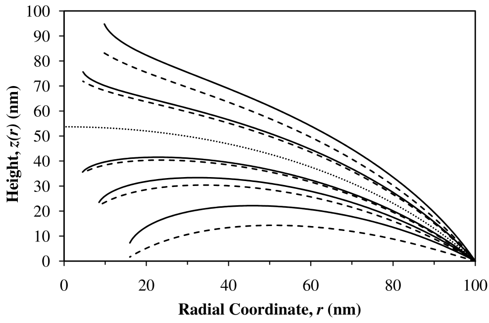
Figure 2: Pinned bubble profiles for various applied loads. The dotted curve is the undeformed bubble (zero load), a full curve is an exact profile, and an adjacent dashed curve is the corresponding linear approximation. Above and below the undeformed profile the loads are $\pm 0.5\,$nN, $\pm 1\,$nN, and $+2\,$nN. The parameters are $s=4$, $\gamma(s)=0.018\,$N/m ($s^{\ddagger}=5$), and $r_{3}=100\,$nm, giving $R_{\mathrm{c}}=120\,$nm, and $z_{\mathrm{c}}=54\,$nm. Each curve terminates at its last stable contact radius.

Figure 2 shows several profiles of deformed bubbles. The exact profile was obtained by numerical integration of the profile equation, Eq. (2.26). Here and below the linear approximation refers to analytic results based the expansion to linear order in the force, in this case Eq. (II.2.3). In the case of the figure, $2\pi r_{1}^{2}\gamma/R_{\mathrm{c}}=0.4\,$nN for $r_{1}=20$ nm. For loads with magnitude much less than this the linear approximation can be guaranteed accurate accurate. It can be seen in the figure that the performance of the linear approximation is rather better than is indicated by this parameter. For larger loads there is a significant discrepancy between the exact and the linear profile. The problem is more acute for extensive than for compressive forces.

II.2.4 Bubble Spring Constant

The various quantities $z$ above were measured relative to the substrate. Now, in the laboratory frame of reference, let $\zeta_{\mathrm{s}}$ be the position of the solid substrate. In this laboratory frame, the position of the tip, the tip contact circle, and the undeformed bubble interface are

$$\zeta_{0}=z_{0}+\zeta_{\mathrm{s}},\;\;\zeta_{1}=z_{1}+\zeta_{\mathrm{s}},\mbox{ and }\zeta_{\mathrm{c}}=z_{\mathrm{c}}+\zeta_{\mathrm{s}},$$ (2.33)

respectively. Initially, the substrate is at $\zeta_{\mathrm{s}}=0$, the tip is just touching the undeformed bubble $\zeta_{0}=z_{\mathrm{c}}$, and the spring attached to the tip is undeflected. Hence in general the deflection is $\delta_{\mathrm{t}}=\zeta_{0}-z_{\mathrm{c}}$, and force exerted by the tip on the bubble is

$$F_{\mathrm{t}}=-k_{\mathrm{t}}\delta_{\mathrm{t}}=-k_{\mathrm{t}}[\zeta_{0}-z_{\mathrm{c}}],$$ (2.34)

where $k_{\mathrm{t}}$ is the tip spring constant.

Now $z_{1}=z_{\mathrm{c}}(r_{1})+\varepsilon(r_{1})$, or

$$\zeta_{1}=\zeta_{\mathrm{c}}(r_{1})+\varepsilon(r_{1}).$$ (2.35)

The amount of bubble deformation at contact is

$$\varepsilon(r_{1})=-k_{\mathrm{bub}}^{-1}F,$$ (2.36)

where $F$ is the force exerted by the bubble. The bubble spring constant is given by the profile equation evaluated at $r_{1}$,

$$k_{\mathrm{bub}}=-2\pi\gamma\left\{\frac{1}{2}\ln\frac{1-\sqrt{1-x_{1}^{2}}}{1+\sqrt{1-x_{1}^{2}}}+\frac{1}{\sqrt{1-x_{1}^{2}}}-C_{3}\right\}^{-1}.$$ (2.37)

This depends upon the two pinning radii. Obviously $R_{\mathrm{c}}>r_{3}>r_{1}$.

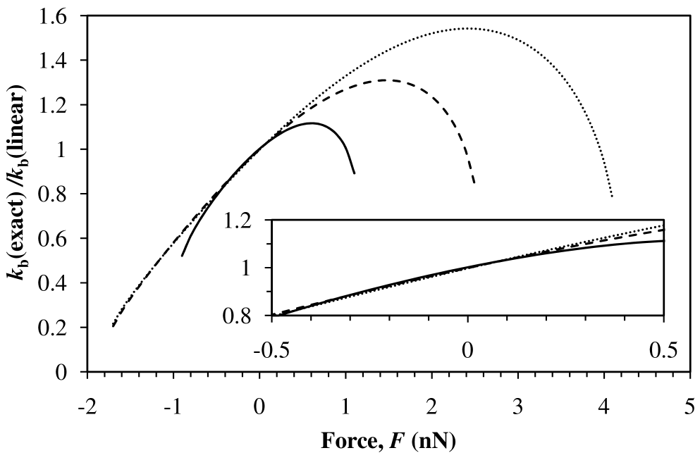
Figure 3: Ratio of exact effective bubble spring constant, $\Delta F/\Delta z(r_{1})$, to linear bubble spring constant $k_{\mathrm{b}}$, Eq. (2.37), as a function of the applied load. The solid, dashed, and dotted curves are for $r_{1}=$ 10, 20, and 30 nm, respectively. Other parameters as in Fig. 2. Each curve terminates at its limits of solution. The inset magnifies the region around zero force.

Figure 3 shows the exact effective spring constant of the bubble, $\Delta F/\Delta z(r_{1})$ obtained from the numerical integration of the profile equation, Eq. (2.26), normalized by the analytic expression obtained from the expansion to linear order in the force, Eq. (2.37). The expansion is valid when $|F|\ll 2\pi\gamma(s)r_{1}^{2}/R_{\mathrm{c}}$. For the conditions in Fig. 3, the right hand side is 0.09, 0.38, and 0.85 nN for $r_{1}=$ 10, 20, and 30 nm, respectively. One can indeed see in the figure that the bubble behaves linearly to within about 20% of the exact value when the loads lie within this bound.

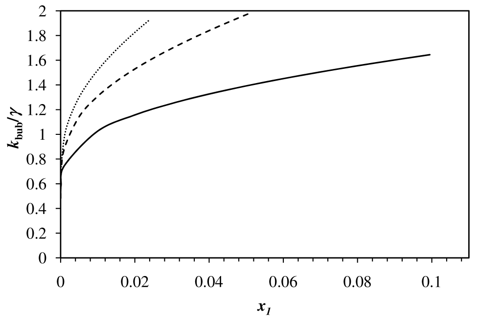
Figure 4: Bubble linear spring constant as a function of tip contact radius $x_{1}\equiv r_{1}/R_{\mathrm{c}}$ for a substrate radius $x_{3}\equiv r_{3}/R_{\mathrm{c}}$ of 0.9 (solid curve), 0.7 (dashed curve), and 0.5 (dotted curve). In each case, the upper limit is $x_{1}^{\mathrm{max}}=[1-\sqrt{1-x_{3}^{2}}]\tan\alpha$, with $\alpha=10^{\circ}$.

Figure 4 shows the ratio of the bubble linear spring constant to the surface tension. It can be seen that the variation is rather weak over the practical range, with the bubble spring constant being not more than a factor of two larger than the surface tension. In general the bubble spring constant is larger than the surface tension unless the contact radius is very small. Clearly, in the absence of specific information about the size of the pinning radii, one will not go too far wrong in taking the liquid-vapor surface tension of the supersaturated interface to be 0.5–1 times the measured bubble spring constant.

In the linear regime, the bubble and tip act as two springs in series. To see this explicitly, consider a change in the position of the substrate, $\Delta\zeta_{\mathrm{s}}$, at constant $r_{1}$ (and $r_{3}$). Since $\Delta r_{1}=0$, the change in contact position must equal the change in tip position, $\Delta\zeta_{1}=\Delta\zeta_{0}$. In the static situation $\Delta F_{\mathrm{t}}=-\Delta F$, and so one has

$$k_{\mathrm{t}}\Delta\zeta_{0} = -k_{\mathrm{bub}}\Delta\varepsilon(r_{1})$$ (2.38)

$$= -k_{\mathrm{bub}}\left[\Delta\zeta_{1}-\Delta\zeta_{\mathrm{c}}(r_{1})\right]$$

$$= -k_{\mathrm{bub}}\left[\Delta\zeta_{0}-\Delta\zeta_{\mathrm{s}}\right].$$

This implies that $\left[k_{\mathrm{t}}+k_{\mathrm{bub}}\right]\Delta\zeta_{0}=k_{\mathrm{bub}}\Delta\zeta_{\mathrm{s}}$, or

$$\frac{\Delta\zeta_{0}}{\Delta\zeta_{\mathrm{s}}}=\frac{k_{\mathrm{bub}}}{k_{\mathrm{t}}+k_{\mathrm{bub}}}.$$ (2.39)

This ratio is less than unity, whereas for a hard surface it would be unity. A measurement of the slope of the deflection versus the drive distance allows the spring constant of the interface to be determined. If the contact radii are known, then the surface tension of the bubble can be estimated.

Alternatively, in terms of the separation between the tip and substrate, $z_{0}\equiv\zeta_{0}-\zeta_{\mathrm{s}}$, one has

$$\frac{\Delta\zeta_{0}}{\Delta z_{0}} = \frac{\Delta\zeta_{0}}{\Delta\zeta_{0}-\Delta\zeta_{\mathrm{s}}}$$ (2.40)

$$= \frac{1}{1-\Delta\zeta_{\mathrm{s}}/\Delta\zeta_{0}}$$

$$= \frac{1}{1-\frac{k_{\mathrm{t}}+k_{\mathrm{bub}}}{k_{\mathrm{bub}}}}$$

$$= \frac{-k_{\mathrm{bub}}}{k_{\mathrm{t}}}.$$

In words, the slope of the deflection versus separation curve equals the negative of the ratio of the bubble and cantilever spring constants.

III Deformed Bubble: Prick Slip

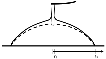
Figure 5: Hemispherical bubble penetrated and deformed by a conical hydrophobic tip (blunt radius $r_{0}$) upon which it slips.

For the case of slip on the tip, the liquid-vapor-solid contact circle is not pinned at $r_{1}$ (see Fig. 5). One now has also to maximize the total entropy with respect to $r_{1}$, taking into account the difference in solid surface energies, $\Delta\gamma\equiv\gamma_{\mathrm{sg}}-\gamma_{\mathrm{sl}}$. This is negative for a hydrophobic tip.

For a macroscopic bubble or droplet on a planar substrate made of the same material as the tip, the equilibrium condition is that the contact angle measured in the liquid phase satisfies $\gamma\cos\theta_{\mathrm{t}}=\Delta\gamma$. This does not hold in the present case of a conical tip penetrating the bubble.

For the present case of slip, the total entropy is

$$S_{\mathrm{tot}}[z] = S_{\mathrm{b}}(N,V,T)-\frac{\gamma}{T}A[z]-\frac{p}{T}V[z]+\frac{\mu}{T}N$$ (3.1)

$$\mbox{ }-\frac{\Delta\gamma}{T}A_{\mathrm{t}}.$$

The surface area of the blunt conical tip inside the bubble is

$$A_{\mathrm{t}}=\frac{\pi r_{1}^{2}}{\sin\alpha}-\frac{\pi r_{0}^{2}}{\sin\alpha}+\pi r_{0}^{2}.$$ (3.2)

The formulae for the volume $V[z]$ and area $A[z]$ were given above and depend upon $r_{1}$. Also recall that $r_{1}-r_{0}=[z_{1}-z_{0}]\tan\alpha$.

Differentiating with respect to the profile (at constant $r_{1}$) gives the Eular-Lagrange equation for the optimum profile, as given above. Differentiating with respect to $r_{1}$, one has $\mathrm{d}r_{1}=\mathrm{d}z_{1}\tan\alpha$, which means that $\delta z(r_{1})=\mathrm{d}r_{1}/\tan\alpha$, and so the extra boundary term in the profile derivative of the area appears, as in §II.2.1. Also, $\mathrm{d}z_{0}=0$. In view of this one has

$$\left.\frac{\partial S_{\mathrm{tot}}}{\partial r_{1}}\right|_{\overline{z}(r)}$$

$$= \left[\frac{\Delta_{p}}{T}\frac{\delta V[z]}{\delta z(r)}-\frac{\gamma}{T}\frac{\delta A[z]}{\delta z(r)}\right]_{\overline{z}(r)}\frac{\partial\overline{z}(r)}{\partial r_{1}}$$

$$\mbox{ }+\left[\frac{2\pi r_{1}^{2}}{\tan\alpha}+2\pi r_{1}\left(z_{0}-\frac{r_{0}}{\tan\alpha}\right)\right]\frac{\Delta_{p}}{T}$$

$$\mbox{ }+\left[2\pi r_{1}\sqrt{1+z^{\prime}(r_{1})^{2}}+\frac{2\pi r_{1}z^{\prime}(r_{1})}{\sqrt{1+z^{\prime}(r_{1})^{2}}\tan\alpha}\right]\frac{\gamma}{T}$$

$$\mbox{ }-\frac{2\pi r_{1}\Delta\gamma}{T\sin\alpha}$$

$$= \frac{2\pi r_{1}}{T}\left\{\left[\frac{2z_{1}}{R_{\mathrm{c}}}+\sqrt{1+z^{\prime}(r_{1})^{2}}+\frac{z^{\prime}(r_{1})/\tan\alpha}{\sqrt{1+z^{\prime}(r_{1})^{2}}}\right]\gamma\right.$$

$$\left.\mbox{ }-\frac{\Delta\gamma}{\sin\alpha}\rule{0.0pt}{17.07182pt}\right\}.$$

Setting this to zero, the trivial solution is $\overline{r}_{1}=0$. The non-trivial solution gives an equation that the profile slope at the optimum radius must satisfy,

$$\frac{\Delta\gamma}{\gamma\sin\alpha}=\frac{2z_{1}}{R_{\mathrm{c}}}+\sqrt{1+z^{\prime}(r_{1})^{2}}+\frac{z^{\prime}(r_{1})/\tan\alpha}{\sqrt{1+z^{\prime}(r_{1})^{2}}}.$$ (3.4)

This replaces the planar contact angle condition.

In the limit $\alpha\rightarrow 0$ this is

$$\frac{\Delta\gamma}{\gamma}=\frac{z^{\prime}(r_{1})}{\sqrt{1+z^{\prime}(r_{1})^{2}}}=\cos\theta_{\mathrm{t}},$$ (3.5)

which is the expected contact angle condition for a cylindrical tip.

The expression for the force ought to be unchanged. Explicitly the force exerted by the bubble on the tip is

$$F = T\frac{\mathrm{d}S_{\mathrm{tot}}}{\mathrm{d}z_{0}}$$ (3.6)

$$= T\left\{\int_{r_{1}}^{r_{3}}\mathrm{d}r\,\left.\frac{\delta S_{\mathrm{tot}}([z],r_{1},z_{0})}{\delta z(r)}\right|_{[\overline{z}],\overline{r}_{1}}\frac{\mathrm{d}\overline{z}(r)}{\mathrm{d}z_{0}}\right.$$

$$\mbox{ }\left.+\left.\frac{\partial S_{\mathrm{tot}}([z],r_{1},z_{0})}{\partial r_{1}}\right|_{[\overline{z}],\overline{r}_{1}}\frac{\mathrm{d}\overline{r}_{1}}{\mathrm{d}z_{0}}\right.$$

$$\mbox{ }\left.+\left.\frac{\partial S_{\mathrm{tot}}([z],r_{1},z_{0})}{\partial z_{0}}\right|_{[\overline{z}],\overline{r}_{1}}\right\}$$

$$= T\left.\frac{\partial S_{\mathrm{tot}}([z],r_{1},z_{0})}{\partial z_{0}}\right|_{[\overline{z}],\overline{z}_{1}}$$

$$= \pi r_{1}^{2}\Delta_{p}+\frac{2\pi r_{1}\gamma z^{\prime}(r_{1})}{\sqrt{1+z^{\prime}(r_{1})^{2}}}.$$

Hence the expression for the profile is unchanged from the stick case, although of course for a non-stick hydrophobic tip, $F<0$.

III.0.1 Algorithms

Recall the equations of for the undeformed profile, Eq. (2.5) et seq. Also recall that in the linear approximation the deformation $\varepsilon(r)\equiv z(r)-z_{\mathrm{c}}(r)$, and its derivative $\varepsilon^{\prime}(r)\equiv z^{\prime}(r)-z_{\mathrm{c}}^{\prime}(r)$, are linearly proportional to the force, Eqs (2.30) and (II.2.3). In view of these one can succinctly write

$$z(r_{1})=z_{\mathrm{c}}(r_{1})-k_{\mathrm{bub}}(r_{1})^{-1}F,$$ (3.7)

and

$$z^{\prime}(r_{1})=z_{\mathrm{c}}^{\prime}(r_{1})+q_{\mathrm{bub}}(r_{1})F.$$ (3.8)

Write $k_{1}\equiv k_{\mathrm{bub}}(r_{1})$ and $q_{1}\equiv q_{\mathrm{bub}}(r_{1})$.

To linear order the optimum contact radius satisfies (recall that $r_{1}-r_{0}=[z(r_{1})-z_{0}]\tan\alpha$)

$$0 = \left[\frac{2z_{1}}{R_{\mathrm{c}}}+\sqrt{1+z^{\prime}(r_{1})^{2}}+\frac{z^{\prime}(r_{1})/\tan\alpha}{\sqrt{1+z^{\prime}(r_{1})^{2}}}\right]\gamma-\frac{\Delta\gamma}{\sin\alpha}$$ (3.9)

$$= \left[\frac{2z_{\mathrm{c}}(r_{1})}{R_{\mathrm{c}}}+\sqrt{1+z^{\prime}_{\mathrm{c}}(r_{1})^{2}}+\frac{z^{\prime}_{\mathrm{c}}(r_{1})/\tan\alpha}{\sqrt{1+z^{\prime}_{\mathrm{c}}(r_{1})^{2}}}\right]\gamma-\frac{\Delta\gamma}{\sin\alpha}$$

$$\mbox{ }-\frac{2\gamma F}{k_{1}R_{\mathrm{c}}}+\left[\frac{z^{\prime}_{\mathrm{c}}(r_{1})\tan\alpha}{\sqrt{1+z^{\prime}_{\mathrm{c}}(r_{1})^{2}}}+\frac{1}{\sqrt{1+z^{\prime}_{\mathrm{c}}(r_{1})^{2}}}\right.$$

$$\left.\mbox{ }-\frac{z^{\prime}_{\mathrm{c}}(r_{1})^{2}}{[{1+z^{\prime}_{\mathrm{c}}(r_{1})^{2}}]^{3/2}}\right]\frac{\gamma q_{1}}{\tan\alpha}F$$

Rearranging this gives explicitly $F(r_{1})$.

Let the equilibrium curve be $\overline{F}(r_{1})$, $\overline{\zeta}_{\mathrm{s}}(r_{1})$. The deflection is $\delta_{\mathrm{t}}=z_{0}+\zeta_{\mathrm{s}}-z_{\mathrm{c}}=-F_{\mathrm{t}}/k_{\mathrm{t}}=F/k_{\mathrm{t}}$. The equilibrium curve in linear approximation can be generated as follows:

• choose $r_{1}$

• calculate $F(r_{1})$, and $z_{0}=z(r_{1})+[r_{0}-r_{1}]/{\tan\alpha}$

• calculate $\zeta_{\mathrm{s}}$ from $F(r_{1})=-F_{\mathrm{t}}=k_{\mathrm{t}}[z_{0}+\zeta_{\mathrm{s}}-z_{\mathrm{c}}]$

• plot deflection, $\delta_{\mathrm{t}}=F(r_{1})/k_{\mathrm{t}}$ versus separation, $z_{0}$.

For the exact, non-linear calculations, one has to specify the load $F$ and calculate the profile $z(r;F)$ by numerical integration from $(r_{3},0)$. For the equilibrium (slip) case, one terminates the profile at the value of $r_{1}$ where the profile has the equilibrium contact angle, Eq. (3.4). In the cases where there are two solutions one chooses the one based on continuity. From the value of $z(r_{1})$, one obtains $z_{0}$ and $\zeta_{\mathrm{s}}$ as in the linear case. One then chooses a new load and repeats the process. For the case of the pinned tip contact line, for each $F$ one instead terminates the profile at the fixed value of $r_{1}$.

III.0.2 Results

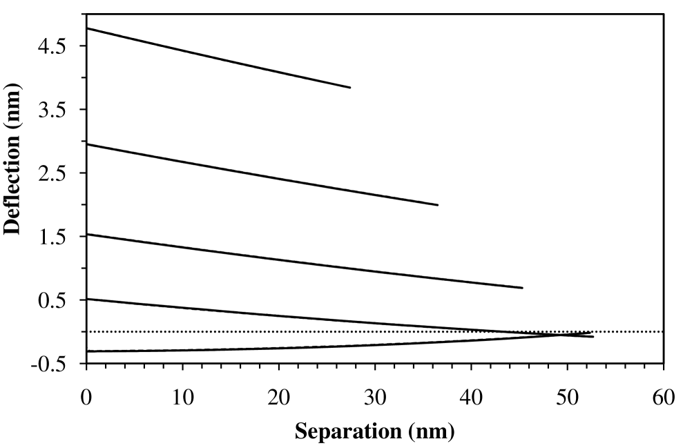
Figure 6: Equilibrium (slip) deflection versus separation curves for a tip penetrating a nanobubble for different tip radii. These are the exact theory for, from bottom to top at contact, blunt tip radii of $r_{0}=$ 0, 20, 30, 40, and 50 nm. The dotted line is a guide to the eye. The tip has $\alpha=10^{\circ}$, $k_{\mathrm{t}}=0.35\,$N/m, and $\Delta\gamma=0\,$N/m or $\theta_{\mathrm{t}}=90^{\circ}$. All other parameters as in Fig. 2.

Figure 6 shows several equilibrium deflection versus separation curves. Equilibrium here and below mean that the contact circle on the tip is free to move. Hence the optimum contact angle that maximizes the entropy is established at each separation. For brevity this is also called slip. The data in the figure is obtained with the exact theory. Results obtained with the linear theory are entirely obscured by the exact curves on the scale of the figure.

In the case of Fig. 6, the tip has been taken to be indifferent to water, $\Delta\gamma=0\,$N/m or $\theta_{\mathrm{t}}=90^{\circ}$, and for the most part the force is repulsive. This corresponds to a positive cantilever deflection and to a compressed bubble, as in Fig. 1 and in the lower half of Fig. 2. The exception is for for the infinitely sharp tip, $r_{0}=0\,$nm, which shows a weak attraction.

It is noticeable that the force curves are almost straight lines, and that their magnitude increases with increasing tip radius. The predominant reason that the force increases with decreasing separation is the cone half angle, which means that the contact radius increases as the tip penetrates further into the bubble with decreasing separation. The main reason that the force becomes more repulsive with increasing end radius $r_{0}$ is that the repulsive pressure contribution is proportional to $r_{1}^{2}$ whereas the often attractive surface tension contribution contains a factor $r_{1}$.

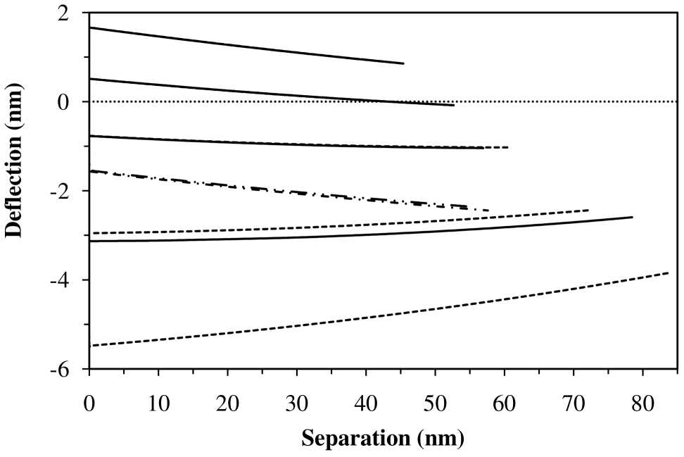
Figure 7: Equilibrium (slip) deflection versus separation for a blunt tip penetrating a nanobubble for different tip surface energies. The solid curves are the exact theory and the dashed curves are the linear theory (obscured in the top three cases), with $r_{0}=20\,$nm and, from bottom to top, $\Delta\gamma=-10.0\,$mN/m ($\theta_{\mathrm{t}}=98^{\circ}$), $-6.3\,$mN/m ($\theta_{\mathrm{t}}=95^{\circ}$), $-2.5\,$mN/m ($\theta_{\mathrm{t}}=92^{\circ}$), $0\,$mN/m ($\theta_{\mathrm{t}}=90^{\circ}$), and $+2.5\,$mN/m ($\theta_{\mathrm{t}}=88^{\circ}$). No exact solution was found for the lowest curve. The dash-dotted curve and the partially obscured dash-double dotted curve are the exact and linear results respectively for $r_{0}=50\,$nm, and $\Delta\gamma=-6.3\,$mN/m ($\theta_{\mathrm{t}}=95^{\circ}$). All other parameters as in Fig. 6.

Figure 7 explores the effect of the tip surface energy difference on the force curves. The conversion of the surface energy difference to a macroscopic tip contact angle uses the Young equation, the saturation value of the surface tension, $\gamma^{\dagger}=0.072\,$N/m, and assumes that the difference in surface energies is unchanged by the level of supersaturation of the solution, $\Delta\gamma=\gamma^{\dagger}\cos\theta_{\mathrm{t}}$.

It can be seen that as the surface energy difference becomes more negative, the force at a given separation becomes increasingly attractive. The penetrated bubble is extended from its undeformed shape (see Fig. 5 and the upper half of Fig. 2). The slope of the almost linear deflection versus separation curves changes from negative to positive for $\Delta\gamma\lesssim-5.0\,$mN/m ($\theta_{\mathrm{t}}\gtrsim 92^{\circ}$), close to where the surface energy difference changes sign, and it becomes increasingly positive as the surface energy difference becomes increasingly negative.

The linear theory becomes increasingly less accurate as the surface energy difference becomes more negative. Indeed, whilst the linear theory produced a solution curve for $\Delta\gamma\leq-10.0\,$mN/m at this $r_{0}=20\,$nm, no exact solution was found (essentially because the bubble ruptured at this contact radius).

Figure 7 also presents the case of $r_{0}=50\,$nm and $\Delta\gamma=-6.3\,$mN/m ($\theta_{\mathrm{t}}=95^{\circ}$). Compared to the same surface energy but for $r_{0}=20\,$nm, one sees that the force is less attractive and as well the slope has decreased, changing from positive to negative. As mentioned above, increasing the contact radius increases the repulsive pressure contribution to the force more than the attractive surface tension contribution. One can conclude that a negative slope is the signature of pressure dominance (large contact radius, small magnitude or positive surface energy difference) whereas a positive slope is the signature of surface energy dominance, (small contact radius, large negative surface energy difference).

In Figs 6 and 7 it can be seen that there is a discontinuous jump from zero deflection prior to contact with the undeformed bubble to a non-zero deflection immediately after contact. This is due to the fact that non-contact forces are neglected in the present model and also to the fact that the end of the tip has been taken to be a disc (ie. perfectly blunt, planar). In the present calculations liquid-vapor interface contact with the flattened end has been excluded. The size of this jump increases with the tip end radius $r_{0}$. Obviously this is an idealized model of the actual tip of the tip, which is actually neither perfectly sharp nor perfectly blunt, and in practice there may be a smooth transition rather than a jump. The cantilever manufacturer typically quotes a tip radius 20–60 nm. Also of course the AFM cantilever tip is generally in the form of a square pyramid rather than the present right circular cone.

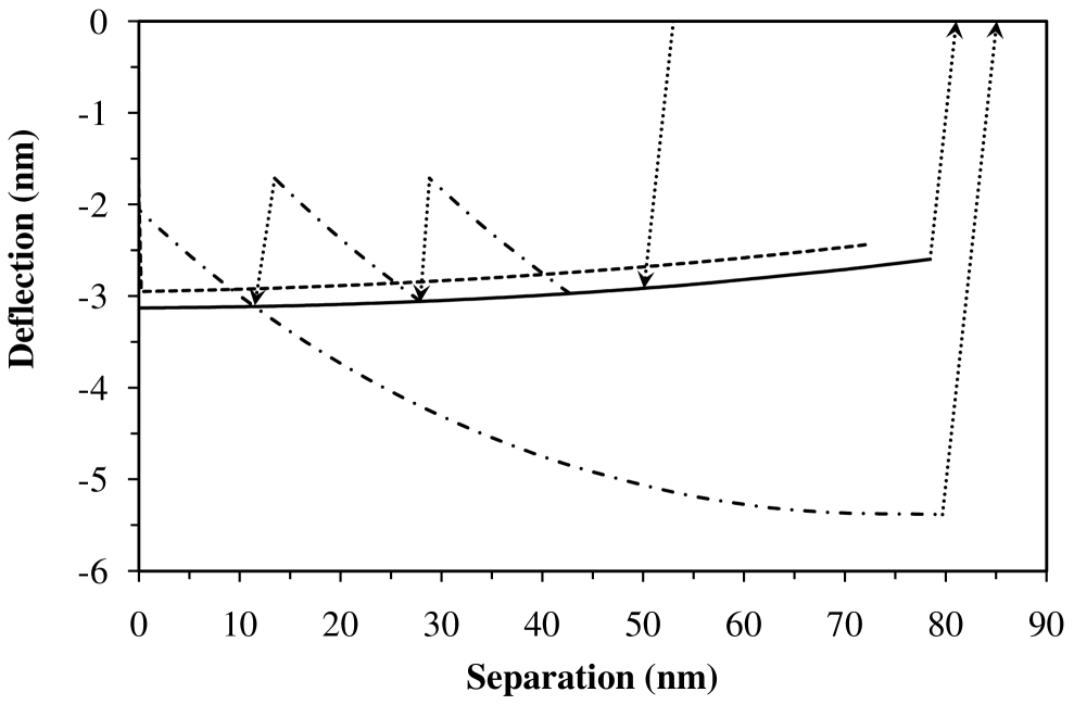
Figure 8: Deflection versus separation for a tip penetrating a nanobubble. The solid curve is the equilibrium slip case using the exact theory, and the parallel dashed curve uses the linear theory. The dash-dotted curve is a stick-slip case using the exact theory, with the pinned contact radii being $r_{1}=$ 26.4, 28.9, and 31.6 nm (chosen more or less arbitrarily). The approach curve overlaps the initial part of the retraction curve on the final stick region. The dotted arrows show cantilever jumps. The final jump out is at the limit of bridging bubble stability for $r_{1}=31.6\,$nm. The blunt tip radius is $r_{0}=20\,$nm, and the difference in tip surface energies is $\Delta\gamma=-6.3\,$mN/m ($\theta_{\mathrm{t}}=95^{\circ}$), with all other parameters Fig. 6.

Figure 8 shows both a slip trajectory and a stick-slip trajectory for a blunt tip, $r_{0}=20\,$nm. The stick branches were chosen more or less randomly, with one eye on aesthetics, one eye on fundamental considerations, and one eye on experimental data. There is no fundamental reason that when the contact line gives way it should jump to, and immediately stick at, the equilibrium position. It could stick prior to reaching the equilibrium position, or it could slip along the equilibrium curve after the jump. One could perhaps argue for a yield stress such that the contact line always slipped when the excess force per unit contact line reached a certain value, but this has not been done here.

The first tip contact line stick has been taken to occur at $r_{1}=26.4\,$nm. For the exact calculation, the initial slope of the stuck branch is -0.078, and the average slope of the entire branch is -0.090. The linear prediction for the slope at this contact radius and surface tension is -0.137.

The second tip contact line stick occurs at $r_{1}=28.9\,$nm, and the exact initial slope is -0.86, and the average slope of the entire branch is -0.95. The linear prediction for the slope at this contact radius is -0.143.

The third tip contact line stick occurs at $r_{1}=31.6\,$nm, and the exact initial slope of the stuck branch is -0.083, and the average slope (extension, into contact) is -0.093. The linear prediction for the slope at this contact radius is -0.150.

For the single stuck branch on retraction, $r_{1}=31.6\,$nm, curvature is quite evident, which graphically indicates that the linear theory is inapplicable. This curvature, including the final flat region, is consistent with the data for the effective exact bubble spring constant in Fig. 3. The vanishing slope is due to the fact that the bubble spring constant tends to zero with increasing bubble extension.

It is evident that in the case treated in Fig. 8, the ratio of the exact slope to the linear slope is about 2:3. This is in agreement with the ratio indicated in Fig. 3 for $F=-1\,$nN. Fitting the linear approximation to measured experimental data where stick is evident, particularly on the extension branch close to the equilibrium curve, can be expected to provide a useful first estimate for the bubble surface tension.

IV Experiment

IV.1 Limitations of Theory

Before analyzing any experimental data, it is worth enumerating the limitations of the present theory.

First, the theory models the tip as a right circular cone, whereas in reality an AFM tip is a rectangular pyramid. Second, it models the tip of the tip as perfectly blunt, a disc of radius $r_{0}$, whereas in reality the tip may be curved from wear. Third, it is assumed that the cross-section of the nanobubble is perfectly circular, which need not be the case if substrate heterogeneity determines where the contact line is pinned. Fourth, it is assumed that the substrate contact line does not alter during the penetration of the nanobubble by the tip.

Fifth, it is assumed that the tip penetrates the nanobubble at the apex, whereas in reality it can penetrate off-axis, either by design or by accident. Sixth, it is assumed that the tip is oriented normal to the substrate, whereas in reality the cantilever and tip are tilted at about 11^∘ in the axial plane. Seventh, it is assumed that the air inside the nanobubble remains in diffusive equilibrium with that in the solution during the force measurement (constant chemical potential), whereas in reality the measurement might be rapid enough for constant number to hold instead.

The fifth and sixth points mean that the predicted normal force on the cantilever has an error that increases with displacement from the central axis of the nanobubble, that the displacement from the central axis varies with the separation and with the deflection of the cantilever during a force measurement (due to the tilt), and that there is a torque on the cantilever due to the asymmetric forces on the tip when it passes through the nanobubble interface off-axis. This nanobubble torque is in addition to the torque that acts in all AFM force measurements on the tip in contact with the hard substrate due to the normal and lateral (friction) forces, which are implicitly included in the photo-diode calibration. Stiernstedt05 ; Attard06 ; Attard13

The limitation summarized in the fifth point can be substantially alleviated by ensuring that the separation at which first contact with the nanobubble occurs is equal to the measured height of the undeformed nanobubble. One is aided in this by the fact that the nanobubble profile is horizontal near the apex. In this case one can be confident that, at least for small cantilever deflections and separations close to initial contact, the tip is penetrating the nanobubble close to the apex, and the calibration factor is correct. In this regime the present calculation of the nanobubble normal force and the neglect of any nanobubble lateral forces or torques, ought to be accurate. The consequences of the seventh point are discussed below on p. IV.2.

In view of these limitations, one ought not to expect the present theory to be able to quantitatively describe every aspect of an individual nanobubble force measurement. The main goal in the first instance is to establish that the nanobubble surface tension is less than the usual air-water surface tension, and if possible to quantify reliably its value for a given solution.

To this end the following protocol was adopted. Primary emphasis was placed on the first pinned region of the measured separation-deflection curve, since this is the one that can be guaranteed closest to the apex. Additional pinned regions were used to confirm the values deduced from the first one.

Since the surface tension that is required to fit a given slope decreases with increasing value of $r_{1}\gtrsim r_{0}$, one can establish an upper bound for the surface tension by specifying the lowest realistic value of $r_{0}$. In view of the specification that a new tip has radius in the range 20–60 nm, fixing for example $r_{0}=20\,$nm should give an upper limit on the surface tension.

Further, as is discussed below on p. IV.2, for a given surface tension and pinned contact radius $r_{1}$, the slope calculated at constant chemical potential is less in magnitude than the slope calculated at constant number. This means that the surface tensions obtained below at constant chemical potential are larger than those that would be required to fit the slopes at constant number. Again one can be confident that the surface tensions obtained here are an upper bound on those for actual nanobubbles.

Since the slope of the pinned regions equals the negative of the ratio of the nanobubble spring constant to the cantilever spring constant, the surface tension can now be determined using the linear theory. The accuracy of this can be checked against the exact theory. From the surface tension and the nanobubble curvature radius determined by tapping mode imaging, the supersaturation ratio is now determined, Eq. (2.1). Using a linear model for the supersaturated surface tension, $\gamma(s)=(s^{\ddagger}-s)\gamma^{\dagger}/(s^{\ddagger}-1)$, Moody03 ; Moody04 ; He05 where $\gamma^{\dagger}=0.072\,$N/m is the saturated surface tension, the spinodal supersaturation ratio $s^{\ddagger}$ can now be determined.

IV.2 Nanobubble 1

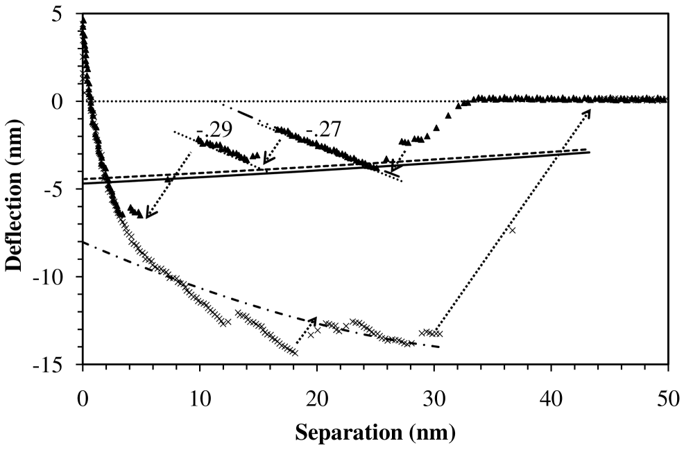
Figure 9: Cantilever deflection versus separation for a SiN tip penetrating a nanobubble on an HOPG substrate on approach (triangles) and retraction (crosses). The cantilever has spring constant $k_{\mathrm{t}}=0.35\,$N/m and conical half-angle $\alpha=10^{\circ}\!$. The undeformed nanobubble has measured height $z_{\mathrm{c}}=33\,$nm and substrate contact radius $r_{3}=108\,$nm, corresponding to a curvature radius $R_{\mathrm{c}}=192\,$nm and a contact angle of $146^{\circ}$. The dotted lines and arrows are guides to the eye, with the adjacent number giving the slope. The full and dashed curves are respectively the calculated exact and linear equilibrium deflection (tip contact line slip) with $r_{0}=10\,$nm, $\gamma=0.040\,$N/m, $s=5.16$, and, $\Delta\gamma=-10.0\,$mN/m (equivalently, $\theta_{\mathrm{t}}=98^{\circ}$). The dash-double dotted line ($r_{1}=10\,$nm, $r_{0}=6\,$nm, obscured), and the dash-dotted curve ($r_{1}=20\,$nm, $r_{0}=10\,$nm), are calculated exact deflections with the tip contact line pinned, using $\gamma=0.044\,$N/m, $s=5.55$.

Figure 9 shows AFM measurements of the force on a cantilever tip due to a single nanobubble. What is plotted is the positional deflection of the cantilever; to obtain the force, multiply by the cantilever spring constant, $k_{\mathrm{t}}=0.35\,$N/m. The first measurably significant deflection occurs at a separation of $z_{0}=32.9\,$nm. This is in good agreement with the height of this particular nanobubble imaged in tapping mode, $z_{\mathrm{c}}=33\,$nm. This suggests that pre-contact forces (van der Waals, electric double layer) are negligible. It also confirms that the measurement was performed in the central region of the nanobubble close to the apex.

The nanobubble profile obtained from the image (not shown) has a contact radius of $r_{3}=108\,$nm, which, with its height, corresponds to a contact angle of $146^{\circ}$. The fact that this contact angle is substantially higher than the contact angle of a macroscopic water drop on HOPG, 64–92^∘,Shin11 ; Li13 is strong evidence that the nanobubble contact rim is pinned.Attard15

In the experimental data just after first nanobubble contact, the positively sloped region, followed by a brief plateau, followed by a small jump to the base of the first marked linear region, are all due to the initial spreading of the nanobubble on the tip of the tip and up its sides. This region is not well-modeled by the present geometry of the tip of the tip as a perfectly planar circular disc. The fact that the deflection is negative in this region indicates that it is favorable for the tip to penetrate the nanobubble, which is to say that the SiNi tip must be hydrophobic, or possibly barely hydrophilic.

The two linear regions with labeled slopes evident in the experimental deflection data on approach confirm that the bubble can have a pinned contact line and behave as a Hookean spring. Since the cone half angle is small, $\alpha=10^{\circ}\!$, to leading order one can take the contact radius used in fitting the slopes to be the same as the radius of the perfectly blunt tip, $r_{1}\approx r_{0}$. The manufacturer’s quoted radius of the tip, 20–60 nm, which might refer to either the tip’s width or else its radius of curvature, can be assumed to be of the same order as $r_{0}$ in the present simple model.

Choosing a contact radius at the lower end of the realistic values, $r_{1}=10\,$nm, a value of $\gamma=0.040\,$N/m gives $k_{\mathrm{b}}/k_{\mathrm{t}}=0.27$, which is the negative of the measured slope of the first linear region. Using Eq. (2.1), this surface tension requires a supersaturation ratio of $s=5.16$ to give a critical radius of $R_{\mathrm{c}}=193\,$nm, equal to that deduced from the tapping mode images of this particular nanobubble. Conversely, choosing the upper limit $r_{1}=50\,$nm, the fitted surface tension is $\gamma=0.015\,$N/m and $s=2.58$. Hence even in the most pessimistic case of smallest contact radius one can see that the nanobubble surface tension, $\gamma=0.040\,$N/m almost a factor of two smaller than the surface tension of the saturated air-water interface, $\gamma=0.072\,$N/m, and that the solution is substantially supersaturated with air, $s=5$.

The just quoted slopes were obtained with the linear theory. Applying the exact non-linear theory with the contact line again pinned at $r_{1}=10\,$nm, the tangent at the start of the dash-double dotted curve in Fig. 9, gives the required slope $-0.27$ using $\gamma=0.044\,$N/m and $s=5.55$. In this case using $r_{0}=6\,$nm shifts the curve laterally to coincide with the measured data. Obviously using larger values of $r_{1}$ will require smaller values of $\gamma(s)$ to fit the slope. There is very little curvature evident in the non-linear curve. The 10% difference in the surface tension between the exact and the linear fits means that the linear theory provides an acceptable estimate of the surface tension from the slope that is both analytic and reliable.

The slope of the second linear region in Fig. 9, $-0.29$, is fitted by $\gamma=0.043\,$N/m using $r_{1}=10\,$nm using the linear theory. Alternatively, the change in contact position of the nanobubble on the tip may be approximated as the change in separation at the base of the two linear regions, $\Delta z_{1}\approx\Delta z_{0}=11\,$nm, assuming that the bubble profile is essentially the same in the two cases, which it would be if the contact line were mobile prior to the start of the pinned regions. The change in contact radius is $\Delta r_{1}=\Delta z_{1}\tan\alpha\approx 2\,$nm. Using this one finds that a single surface tension (to better than 0.03%) $\gamma=0.0402\,$N/m gives a slope of -0.27 using $r_{1}=10\,$nm, and a slope of -0.29 using $r_{1}=12\,$nm. In the case of $r_{1}=50\,$nm and $r_{1}=52\,$nm, the two slopes are given by a single surface tension with a slightly worse variance of $2\%$. This tends to suggest that the smaller contact radius is more applicable, but this is by no means conclusive. In any case, that a single surface tension combined with the geometry of the tip fits the two slopes supports the model and the value of the surface tension.

Here and below the calculations are performed at constant chemical potential, which is computationally convenient. Although there is strong evidence (see below) that the nanobubble is in diffusive equilibrium with the solution over the time of the series of force measurements, it is unclear whether it is best to model each force measurement as at constant chemical potential or as at constant number. For the purposes of comparison, some exact calculations have been carried out at constant number. Using a surface tension of $\gamma(s)=0.044\,$N/m, at a pinned radius of $r_{1}=10\,$nm the tangent at zero force at constant chemical potential is -0.30, compared to -0.41 at constant number. Using instead $r_{1}=20\,$nm and the same surface tension, the tangent at zero force at constant chemical potential is -0.40, compared to -0.62 at constant number. One sees that the slope has a higher magnitude at constant number, and that it increases relatively more rapidly with contact radius. Hence one would require smaller surface tensions to fit the measured slopes if one used constant number. The calculations here and below are at constant chemical potential, and so the surface tensions obtained represent an upper bound on the actual nanobubble surface tension.

The two almost horizontal curves in Fig. 9 are the calculated exact and linear equilibrium curves, which assume that the contact line is mobile on the tip. The good agreement between the linear and the exact calculations is somewhat better than that for the predicted effective bubble spring constant. Both equilibrium calculations use $r_{1}=10\,$nm, $\gamma=0.04\,$N/m, and $s=5.16$. In addition a surface energy difference of $\Delta\gamma=-10.0\,$mN/m was fitted, which corresponds to a macroscopic contact of water on a planar SiNi substrate of $\theta_{\mathrm{t}}=98^{\circ}$. This is slightly hydrophobic. The criterion for the fit, which was done by eye, was that the curve should pass close to the base of the two linear regions. (For reasons that are discussed below, the end point of the final jump was not included in the fit.) Since the cantilever jumps to these bases, the nanobubble at contact must also be moving along the tip, and so it can probably be assumed that the contact position is the equilibrium one. Of course the contact line may become pinned at the end of the jump prior to achieving its equilibrium position, so this fit may underestimate the magnitude of the surface energy difference. Also, using a larger contact radius would require a smaller in magnitude value for the fit. Fortunately, the surface tension obtained by fitting the slopes of the linear regions is not affected by the tip solid surface energies.

From the fitted value of the surface tension at $r_{1}=10\,$nm, $\gamma=0.040\,$N/m, and the measured nanobubble curvature radius, $R_{\mathrm{c}}=193\,$nm, which is equal to the critical radius, Eq. (2.1), the supersaturation ratio can be deduced to be $s=5.2$. The linear model for the supersaturated surface tension is $\gamma(s)=(s^{\ddagger}-s)\gamma^{\dagger}/(s^{\ddagger}-1)$, where $\gamma^{\dagger}=0.072\,$N/m is the saturated surface tension, and $s^{\ddagger}$ is the spinodal saturation ratio. This has been shown to fit the available computer simulation data reasonably accurately.Moody03 ; Moody04 ; He05 These computer simulations give $s^{\ddagger}\approx$4–6 for a Lennard-Jones fluid, depending on the temperature. The present fit, $\gamma(5.2)=0.040\,$N/m, gives the spinodal supersaturation ratio $s^{\ddagger}=10.4$. Alternatively, at $r_{1}=50\,$nm, the linearly fitted supersaturated surface tension $\gamma=0.015\,$N/m requires $s=2.6$ to give the measured nanobubble curvature radius, and corresponds to $s^{\ddagger}=3.0$ in the linear model.

Also shown in Fig. 9 is the calculated exact (ie. non-linear) deflection on extension with the contact radius pinned at $r_{1}=20\,$nm. The value of the contact radius was chosen so that the calculated curve fitted by eye the measured data at the end of the retraction branch. This calculation used the non-linear fitted value $\gamma=0.044\,$N/m and $s=5.55$, and also $r_{0}=10.3\,$nm, which shifts the curve laterally. The consistency of this with the exact fit to the slope $-0.27$ ($r_{1}=10\,$nm and $r_{0}=6.2\,$nm) is probably already acceptable; with a little optimization of $r_{1}$ it could doubtless be made even better. It is also undoubtable that larger values of $r_{1}$ and $r_{0}$ and smaller values of $\gamma(s)$ could also fit both the slope of the pinned regions on approach and the flattened region on retraction. The conclusion that one can draw is that for separations $z_{0}\gtrsim 20\,$nm the retraction data can be described by the pinned nanobubble model using parameters consistent with what was deduced from the slopes of the pinned approach data.

For separations $z_{0}\lesssim 20\,$nm on retraction, and $z_{0}\lesssim 3\,$nm on approach, the data in Fig. 9 is not described by either the pinned or the mobile contact line theory. Similar steep curved regions have been observed in a number of other AFM nanobubble measurements, albeit for colloid probes rather for tips. Carambassis98 ; Tyrrell02 The origin of this particular behavior is unclear. Because of the coincidence of approach and retraction here, this is clearly an equilibrium, non-dissipative phenomenon. Calculations show that it is not due to elastic deformation of the substrate (not shown).Attard92 ; Attard01b It might be due to torque on the cantilever, although measurements across the nanobubble indicate that this is in general negligible. That the curve is much steeper at $F=0$ than the clearly pinned regions suggests that it is not due to pinning of the contact line, unless the pinned contact radius had increased very substantially. The apparently contiguous flat region $r\gtrsim 20\,$nm on retraction is similar to the non-linear calculations of the force due to pinning of a highly extended nanobubble with small contact radius. Obviously whatever the origin of this behavior, it could be simply additive to the force due to the pinned (or slipping) contact line since the nanobubble force is always present. Because of the uncertainty as to the origin of this force close to contact it has been neglected in fitting the nanobubble.

The measurements in Fig. 9 were part of a sequence of twelve successive force measurements across this particular nanobubble (not shown). The number, position, and extent of the linear regions could differ between force measurements, presumably because contact line stick and slip are stochastic events, but the slopes were unchanged. This suggests that torque on the cantilever due to off-apex penetration has negligible effect. Tapping mode images before and after the sequence of force measurements show that the nanobubble itself was unchanged in size and shape by the force measurements. This is strong evidence that the nanobubble is thermodynamically stable, and that even penetrating it a dozen times with the cantilever tip did not destroy or alter it. It is also evidence that the nanobubble is pinned at it contact rim. In several other series of measurements, up to a hundred force measurements were performed on a single nanobubble, interspersed with several AFM tapping mode images, and no significant change in the nanobubble was observed in any case.

IV.3 Nanobubble 2

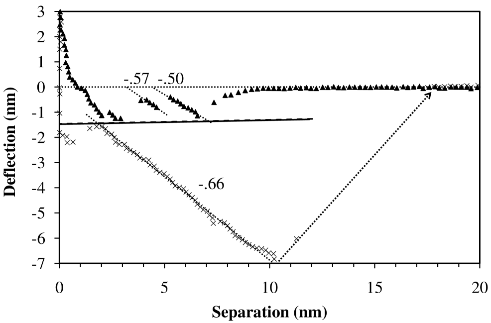
Figure 10: Measured cantilever deflection versus separation for a nanobubble (curves and lines as in preceding figure; different nanobubble, cantilever, and solution). The cantilever has spring constant $k_{\mathrm{t}}=0.24\,$N/m, and conical half-angle $\alpha=10^{\circ}\!$. The undeformed nanobubble has measured height $z_{\mathrm{c}}=9.6\,$nm and substrate contact radius $r_{3}=82.5\,$nm, corresponding to a curvature radius $R_{\mathrm{c}}=359\,$nm and a contact angle of $167^{\circ}$. The calculated equilibrium exact (solid) and linear (dashed, obscured) curve use $r_{0}=10\,$nm, $\gamma=0.041\,$N/m, $s=3.3$, and $\Delta\gamma=+1.3\,$mN/m (equivalently, $\theta_{\mathrm{t}}=89^{\circ}$).

Figure 10 shows results for another nanobubble in a different solution, with stick-slip behavior evident. Assuming an initial tip contact radius of $r_{1}=10\,$nm, the measured slope $-0.50$ corresponds to a surface tension of $\gamma(s)=0.041\,$N/m (linear approximation). Using instead $r_{1}=20\,$nm gives $\gamma(s)=0.028\,$N/m. Larger contact radii require even smaller surface tension to yield this slope. Exact calculations differ by less than 1% from the linear results for the bubble spring constant in this regime.

The second pinned region with slope -0.57 corresponds to $\gamma(s)=0.047\,$N/m using $r_{1}=10\,$nm, and to $\gamma(s)=0.032\,$N/m using $r_{1}=20\,$nm. The third pinned region with slope -0.66 corresponds to $\gamma(s)=0.054\,$N/m using $r_{1}=10\,$nm, and to $\gamma(s)=0.037\,$N/m using $r_{1}=20\,$nm.

From the point at which the pinned regions extrapolate to zero deflection, one can deduce the value of the pinned radius $r_{1}$ for a specified value of the tip radius $r_{0}$. However, it is not possible to find a single value of $r_{0}$ which yields a single surface tension when all three slopes are fitted. For example, fixing $r_{0}=10\,$nm, one finds that the three slopes -0.50, -0.57, and -0.66 correspond to $r_{1}=$ 10.9, 11.1, and 11.7 nm, and to $\gamma(s)=$ 0.039, 0.045, and 0.050 N/m, respectively. There is nothing wrong with $r_{1}$ increasing with each successive pinning event as the tip penetrates the nanobubble, but one would have hoped for a single surface tension. The best that can be done (ie. minimizing the sum of the relative standard deviations in surface tension and in tip radius), yields $r_{0}=12.323\pm.001\,$nm and $\gamma(s)=$0.036, 0.041, and 0.046 N/m, respectively. Possibly doing the calculations at constant number rather than the present constant chemical potential might yield more consistent results (see p. IV.2). Or possibly the problem is related to the unknown origin of the steep hook at small separations discussed on p. IV.2. In any case, the preferred value of surface tension is the one taken from the very first pinned region, since this lies closest to the tip of the tip of the cantilever and to zero force.

The surface tension obtained using $r_{1}=10\,$nm, $\gamma(s)=0.041\,$N/m, and the nanobubble radius of curvature $R_{\mathrm{c}}=359\,$nm correspond to a supersaturation value of $s=3.3$. Using this in the linear model for the supersaturated surface tension gives a spinodal supersaturation ratio of $s^{\ddagger}=6.3$. Using instead $r_{1}=20\,$nm, $\gamma(s)=0.028\,$N/m, correspond to a supersaturation value of $s=2.6$. and a spinodal supersaturation ratio of $s^{\ddagger}=3.6$.

Figure 10 also shows equilibrium calculations using $r_{0}=10\,$nm, $\gamma(s)=0.041\,$N/m, and $s=3.3$. The value of the surface energy difference, $\Delta\gamma=+1.3\,$mN/m (equivalently, $\theta_{\mathrm{t}}=89^{\circ}$) was chosen so that the curves passed through the base of the first pinned region. The exact and the linear calculations are almost indistinguishable.

IV.4 Nanobubbles 3 and 4

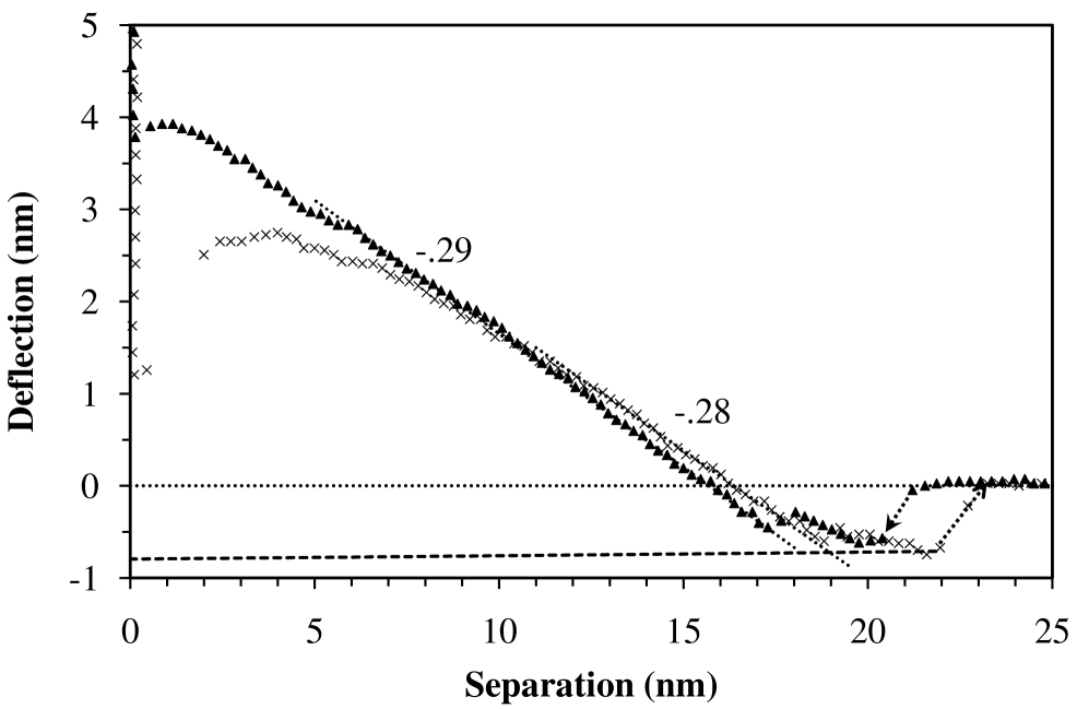
Figure 11: Measured cantilever deflection versus separation for a nanobubble (curves and lines as in preceding figure; different cantilever, solution, and nanobubble). The cantilever has spring constant $k_{\mathrm{t}}=0.35\,$N/m, and conical half-angle $\alpha=10^{\circ}\!$. The undeformed nanobubble has measured height $z_{\mathrm{c}}=19.5\,$nm and substrate contact radius $r_{3}=205\,$nm, corresponding to a curvature radius $R_{\mathrm{c}}=1087\,$nm and a contact angle of $169^{\circ}$. The dashed curve is equilibrium (slip) linear theory with $r_{0}=20\,$nm, $\gamma=0.037\,$N/m, $s=1.68$, and $\Delta\gamma=+3.8\,$mN/m (equivalently, $\theta_{\mathrm{t}}=87^{\circ}$).

Figure 11 shows yet another nanobubble measurement. The AFM fluid cell was flushed with ethanol and then water which means that there was likely exothermic heating. The undeformed nanobubble has apex height $z_{\mathrm{c}}=19.5\,$nm with the first indication of a force occurring at a separation of 21.9 nm. The nanobubble was re-imaged after 47 force measurements and the apex height was $z_{\mathrm{c}}=21.5\,$nm, and the substrate contact radius was $r_{3}=215\,$nm, which correspond to a curvature radius $R_{\mathrm{c}}=1081\,$nm. Again this is unambiguous evidence that the nanobubble is thermodynamically stable.

The two linear regions measured in the figure, one each on extension and retraction, may be attributed to stick. Assuming a contact radius of $r_{1}=20\,$nm, the slope $-0.28$ corresponds to $\gamma(s)=0.037\,$N/m. Alternatively for this slope, $r_{1}=10\,$nm corresponds to $\gamma(s)=0.048\,$N/m. and $r_{1}=50\,$nm $\gamma(s)=0.022\,$N/m. The exact and linear bubble spring constants agree to better than 0.05% in this regime.

The value $\gamma(s)=0.037\,$N/m, and the nanobubble radius of curvature $R_{\mathrm{c}}=1070\,$nm correspond to a supersaturation value of $s=1.7$. Using this in the linear model for the supersaturated surface tension gives a spinodal supersaturation ratio of $s^{\ddagger}=2.4$. Alternatively, $\gamma(s)=0.048\,$N/m corresponds to $s=1.9$ and $s^{\ddagger}=3.6$.

One can assume that the cantilever initially jumps in to the equilibrium slip position, which is supported by the flat nature of the deflection curve and the coincidence of approach and retraction. Assuming again a flattened conical tip with $r_{0}=20\,$nm, these data are well-fitted using $\gamma(s)=0.037\,$N/m, $s=1.7$, and $\Delta\gamma=+3.8\,$mN/m, which would correspond to a macroscopic contact angle of water on silicon nitride of $\theta_{\mathrm{t}}=87^{\circ}$. The validity of the fit is supported by the coincidence of the jump-out separation and the end of the stability of the extended nanobubble. It can be mentioned that a virtually identical equilibrium slip curve can be obtained for $r_{0}=50\,$nm, with $\gamma(s)=0.022\,$N/m, $s=1.41$, and with $\Delta\gamma=+2.3\,$mN/m, which would correspond to a macroscopic contact angle of water on silicon nitride of $\theta_{\mathrm{t}}=88.2^{\circ}$. The equilibrium data can also be fitted by $r_{0}=10\,$nm, with $\gamma(s)=0.048\,$N/m, $s=1.9$, and with $\Delta\gamma=+2.5\,$mN/m, ($\theta_{\mathrm{t}}=88^{\circ}$).

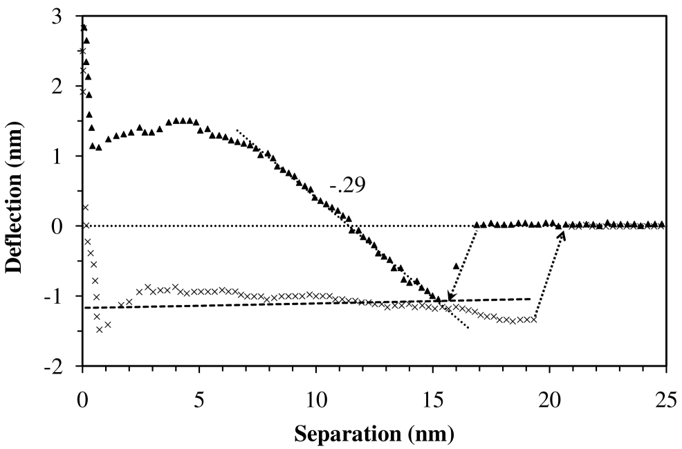
Figure 12: Measured cantilever deflection versus separation for a nanobubble (same cantilever and solution as in the preceding figure; different nanobubble). The undeformed nanobubble has measured height $z_{\mathrm{c}}=15.9\,$nm and substrate contact radius $r_{3}=174\,$nm, corresponding to a curvature radius $R_{\mathrm{c}}=970\,$nm and a contact angle of $170^{\circ}$. The dashed curve is equilibrium (slip) linear theory with $r_{0}=20\,$nm, $\gamma(s)=0.035\,$N/m, and $s=1.72$, and $\Delta\gamma=+2.5\,$mN/m (equivalently, $\theta_{\mathrm{t}}=88^{\circ}$).

Figure 12 shows another nanobubble in the same solution as Fig. 11. Despite the differences in height and contact radii, the two nanobubble have about the same radius of curvature ($R_{\mathrm{c}}=1087\,$nm there and $970\,$nm here). This is consistent with the level of supersaturation of the solution being unchanged and with the nanobubbles being in diffusive equilibrium. Likewise, one would expect the surface tension to be unchanged, and this is confirmed by the fact that the slope of the linear pinned regions are about the same ($-0.28$ there and $-.29$ here).

Using a contact radius of $r_{0}=20\,$nm, the slope of the stick region in extension in Fig. 12 of $-0.29$ corresponds to a surface tension of $\gamma=0.035\,$N/m, a supersaturation ratio of $s=1.72$, and a spinodal supersaturation ratio of $s^{\ddagger}=2.4$. The minimum of the extension curve touches a calculated equilibrium slip curve for $\Delta\gamma=+2.5\,$mN/m (equivalently, $\theta_{\mathrm{t}}=88^{\circ}$).

Using instead a contact radius of $r_{0}=50\,$nm, the slope of the stick region in extension in Fig. 12 of $-0.29$ corresponds to $\gamma(s)=0.020\,$N/m, $s=1.42$, $s^{\ddagger}=1.58$. Fitting the minimum of the extension curve gives $\Delta\gamma=+1.3\,$mN/m (equivalently, $\theta_{\mathrm{t}}=89^{\circ}$).

Using instead a contact radius of $r_{0}=10\,$nm, the slope of $-0.29$ corresponds to $\gamma(s)=0.046\,$N/m, $s=1.95$, $s^{\ddagger}=3.61$. Fitting the minimum of the extension curve gives $\Delta\gamma=+3.8\,$mN/m (equivalently, $\theta_{\mathrm{t}}=87^{\circ}$).

It should be mentioned that the slope of the stick region was checked against that given by the exact theory and the agreement was better than 1%. The origin of the non-linearity and peak in the putative pinned region in Fig. 12 (and in Fig. 11) is unclear, although one could speculate that the contact line might be moving with a finite velocity in these regions.

The slight negative slope in the putative equilibrium curve here in Fig. 12 is difficult to reproduce in the theoretical calculations.

V Conclusion

Table 1: Measured and Deduced Properties of Nanobubbles and Solutions ($r_{0}=10\,$nm).

Figure	$k_{\mathrm{t}}$	$r_{3}$	$z_{\mathrm{c}}$	$R_{\mathrm{c}}$	$\gamma(s)$	$s$	$s^{\ddagger}$	$\theta_{\mathrm{t}}$
	(N/m)	(nm)	(nm)	(nm)	(N/m)			(deg.)
9	0.35	108	33	192	0.040	5.2	10.4	98
10	0.24	82.5	9.6	359	0.041	3.3	6.3	89
11∗	0.35	205	19.5	1087	0.047	1.9	3.6	87
12∗	0.35	174	15.9	970	0.046	2.0	3.6	88

The present paper gives analytic expressions for the nanobubble spring constant that allow its surface tension to be obtained from the slope of the pinned regions in a force-separation AFM measurement. Expressions are also given that allow the difference in tip surface energies (tip contact angle) to be obtained from an equilibrium part of the force curve.

The present fits to the experimental data do not give enough information to pin down the value of the blunt tip radius $r_{0}$. However, sensible results are generated by assuming a tip and contact radius $r_{0}=r_{1}=10\,$nm (Table 1). This is at the lower end of the range of a typical AFM tapping mode cantilever tip, 20–60 nm. A high value of the radius, $r_{0}=r_{1}=50\,$nm gave quite low values of the surface tension, supersaturation ratio, and spinodal supersaturation ratio.

The most reliable data appears to be that of Fig. 9. In this case the two pinned regions both appear to begin from the equilibrium curve, which means that the change in contact radius can be found from the change in separation of the starts. Hence one has three knowns (the two slopes and the change in contact radius) and three unknowns (the surface tension and the two contact radii). Solving this system yields the contact radii $r_{1}=9.4\,$nm and $r_{1}^{\prime}=11.4\,$nm, and also $\gamma(s)=0.041\,$N/m, $s=5.2$ and $s^{\ddagger}=10.8$. Unfortunately the other figures do not have pinned regions starting from the equilibrium curve and so the change in contact radius cannot be readily deduced.

The estimates of the surface energy difference and macroscopic tip contact angle are based on the equilibrium curves and are not so reliable. Little more can be said than that the contact angle is close to $90^{\circ}$.

Likewise the estimate of the value of the spinodal supersaturation ratio has limited reliability because of the simplicity of the linear supersaturated surface tension model. It is nonetheless consoling that it comes out to be of the same order as has been found in computer simulations of a Lennard-Jones fluid.Moody03 ; Moody04 ; He05

One of the purposes of this study was to establish experimentally that the surface tension of nanobubbles was less than that of saturated water. The surface tension is obtained from the slope of the pinned regions and does not rely upon the surface energy difference nor the spinodal supersaturation ratio. The greatest uncertainty concerns the tip radius, and to this end it is better to use a low value, since this overestimates the surface tension. (Doing the calculations at constant chemical potential rather than at constant number further overestimates the surface tension.) Hence the data in Table 1 for $r_{0}=10\,$nm, which give $0.04\lesssim\gamma(s)\lesssim 0.05\,$N/m, are most likely an upper bound on the nanobubble surface tension. The nanobubble surface tension is substantially reduced from that of the saturated air water interface, $\gamma^{\dagger}=0.072\,$N/m.

The solution supersaturation ratios are deduced to be in the range $1.9\lesssim s\lesssim 5.2$ using $r_{0}=10\,$nm. These values appear realistic given the fact that a 15^∘C change in temperature is enough to change the solubility of CO₂ by a factor of two.

It is clear that in order to reliably obtain the dependence of the surface tension on the supersaturation ratio one needs to know the contact radius to within a few nanometers. In contrast, in order to prove that the solution is supersaturated and that the surface tension is less than the saturated value one does not need to know the tip radius precisely.

On this basis one can conclude that the present analysis of these experimental measurements on nanobubbles explicitly confirm what is required by thermodynamics: for nanobubble equilibrium the solution must be supersaturated, and a supersaturated solution has a lower surface tension than a saturated solution.Moody02 ; Moody03

In future experimental studies, electron micrography or AFM inverse imaging could be used to get an independent estimate of the cross-sectional radius of the tip. Also, attempts could be made to explicitly control or to measure the supersaturation of the solution.

Acknowledgement. The AFM data used here was supplied by Liwen Zhu. I thank her and Chiara Neto for interesting discussions during an earlier stage of the project.

References

- (1) J. L. Parker, P. M. Claesson, and P. Attard, J. Phys. Chem. 98, 8468 (1994).
- (2) A. Carambassis, L. C. Jonker, P. Attard, and M. Rutland, Phys. Rev. Lett. 80, 5357 (1998).
- (3) J. W. G. Tyrrell and P. Attard, Phys. Rev. Lett. 87, 176104 (2001).
- (4) J. W. G. Tyrrell and P. Attard, Langmuir 18, 160 (2002).
- (5) J. Wood and R. Sharma, Langmuir 11, 4797 (1995).
- (6) L. Meagher and V. S. J. Craig, Langmuir 10, 2736 (1994).
- (7) R. F. Considine, R. A. Hayes, and R. G. Horn, Langmuir 15, 1657 (1999).
- (8) J. Mahnke, J. Stearnes, R. A. Hayes, D. Fornasiero, and J. Ralston, Phys. Chem. Chem. Phys. 1, 2793 (1999).
- (9) N. Ishida, M. Sakamoto, M. Miyahara, and K. Higashitani, Langmuir 16 5681 (2000).
- (10) E. E. Meyer, Q. Lin, and J. N. Israelachvili, Langmuir 21, 256 (2005).
- (11) H. Stevens, R. F. Considine, C. J. Drummond, R. A. Hayes, and P. Attard, Langmuir 21, 6399 (2005).
- (12) M. Holmberg, A. Kühle, J. Garnaes, K. A. Mørc, and A. Boisen, Langmuir 19, 10510 (2003).
- (13) A. Simonsen, P. Hansen, and B. Klosgen, J. Colloid Interface Sci. 273, 291 ( 2004).
- (14) X. H. Zhang, X. D. Zhang, S. T. Lou, Z. X. Zhang, J. L. Sun, and J. Hu, Langmuir 20, 3813 ( 2004).
- (15) X. H. Zhang, G. Li, N. Maeda, and J. Hu, Langmuir 22, 9238 ( 2006).
- (16) X. H. Zhang, N. Maeda, and V. S. J. Craig, Langmuir 22, 5025 (2006).
- (17) S. Yang, S. M. Dammer, N. Bremond, H. J. W. Zandvliet, E. S. Kooij, and D. Lohse, Langmuir 23, 7072 (2007).
- (18) P. Attard, Eur. Phys. J. Special Topics 223, 893 (2014).
- (19) M. P. Moody and P. Attard, J. Chem. Phys. 117, 6705 (2002).
- (20) M. P. Moody and P. Attard, Phys. Rev. Lett. 91, 056104 (2003).
- (21) P. Attard, arXiv:1503.04365 (2015).
- (22) J. W. Cahn and J. E. Hilliard, J. Chem. Phys. 28, 258 (1959).
- (23) D. w. Oxtoby and R. Evans, J. Chem. Phys. 89, 7521 (1988).
- (24) D. W. Oxtoby, Acc. Chem. Res. 31, 91 (1998).
- (25) S. M. Thompson, K. E. Gubbins, J. P. R. B. Walton, R. A. R. Chantry, and J. S. Rowlinson, J. Chem. Phys. 81, 530 (1984).
- (26) M. P. Moody and P. Attard, J. Chem. Phys. 120, 1892 (2004).
- (27) S. He and P. Attard, Phys. Chem. Chem. Phys. 7, 2928 (2005).
- (28) P. Attard and S. J. Miklavcic, Langmuir 17, 8217 (2001). Erratum: 19, 2532 (2003).
- (29) J. S. Rowlinson and B. Widom, Molecular Theory of Capillarity, (Oxford University Press, Oxford, 1982).
- (30) P. Attard, Thermodynamics and Statistical Mechanics: Equilibrium by Entropy Maximisation, (Academic Press, London, 2002).
- (31) P. Attard, Langmuir 12, 1693 (1996).
- (32) P. Attard, Langmuir 16, 4455 (2000).
- (33) J. Stiernstedt, M. W. Rutland, and P. Attard, Rev. Sci. Instrum. 76, 083710 (2005). Erratum, Rev. Sci. Instrum. 77, 019901 (2006).
- (34) P. Attard, T. Pettersson, and M. W. Rutland, Rev. Sci. Instrum. 77, 116110 (2006).
- (35) P. Attard, arXiv:1302.6630 (2013).
- (36) Y. J. Shin et al., arXiv:1103.4667
- (37) Z. Li et al. Nature Materials 12, 925 (2013).
- (38) P. Attard and J. L. Parker, Phys. Rev. A 46, 7959 (1992).
- (39) P. Attard, Langmuir 17, 4322 (2001).