Finite-Temperature Gutzwiller Approximation from Time-Dependent
Variational Principle

Abstract

We develop an extension of the Gutzwiller approximation to finite temperatures based on the Dirac-Frenkel variational principle. Our method does not rely on any entropy inequality, and is substantially more accurate than the approaches proposed in previous works. We apply our theory to the single-band Hubbard model at different fillings, and show that our results compare quantitatively well with dynamical mean field theory in the metallic phase. We discuss potential applications of our technique within the framework of first principle calculations.

The Gutzwiller approximation (GA) Gutzwiller (1963, 1964, 1965) is a very useful tool in order to study the ground state of complex strongly correlated electron systems. This important many-body technique has been also formulated and implemented in combination with density functional theory (DFT), Hohenberg and Kohn (1964) e.g., in the LDA+GA approach, Deng et al. (2009); Ho et al. (2008); Lanatà et al. (2015) which has been applied successfully to many real materials. Lu et al. (2013); Wang et al. (2010a); Schickling et al. (2012); Zhou and Wang (2010); Julien and Bouchet (2006); Lanatà et al. (2013a, b); Lanatà et al. (2014, 2015) For strongly correlated metals, the accuracy of the GA is comparable with dynamical mean field theory (DMFT), Georges et al. (1996); Anisimov and Izyumov (2010) even though the GA is much less computationally demanding. This property makes it an ideal theoretical tool, as numerical speed is essential for the purpose of studying and discovering new materials.

In order to study several temperature-dependent phenomena, such as structural and magnetic transitions and coherence-incoherence crossovers, it would be highly desiderable to have at our disposal an extension to finite temperatures of the GA as accurate as the ordinary theory for the ground state. In fact, this would enable us to study these properties also for correlated systems so complex to be out of the reach of the presently available methods, such as DMFT.

An extension of the GA to finite temperatures has been previously proposed in Refs. Wang et al., 2010b; Sandri et al., 2013. This approximation scheme is based on an exact entropy inequality which enables to calculate an upper bound to the free energy, Sandri et al. (2013) and minimize it numerically. Of course, underestimating the entropy using an entropy inequality — rather than calculating it exactly — constitutes a source of approximation not present in the ordinary zero-temperature GA. In particular, it has been shown that this additional source of approximation generates a few pathologies of the theory, such as giving a negative entropy at low temperatures. Wang et al. (2010b); Sandri et al. (2013)

In this work we introduce an extension of the GA to finite temperatures based on the Dirac-Frenkel variational principle P. A. M. (1930); Frenkel (1934); DeAngelis and Gatoff (1991) and, in particular, on the time-dependent GA theory Schirò and Fabrizio (2010); Lanatà and Strand (2012) (that we generalize to mixed states). Our method does not rely on any entropy inequality, but only on the variational principle and the Gutzwiller approximation — which are the same approximations done in the ordinary zero-temperature GA. Consequently, as we are going to show, our theory improves considerably the method of Refs. Wang et al., 2010b; Sandri et al., 2013, and gives results in good quantitative agreement with DMFT for correlated metals, even though it is much less computationally demanding.

Imaginary-time evolution.— Let us consider a generic system of correlated electrons represented by a Hamiltonian $\hat{\mathcal{H}}$, and define the imaginary-time evolution of a given initial density matrix $\mathcal{\hat{\rho}}_{0}$ as follows:

$$\mathcal{\hat{\rho}}(\tau)=e^{-\hat{\mathcal{H}}\tau}\,\mathcal{\hat{\rho}}_{0}\,e^{-\hat{\mathcal{H}}\tau}\,,$$ (1)

i.e., according to the following differential equation:

$$\partial_{\tau}\mathcal{\hat{\rho}}(\tau)=-(\hat{\mathcal{H}}\mathcal{\hat{\rho}}(\tau)+\mathcal{\hat{\rho}}(\tau)\hat{\mathcal{H}})\equiv-\{\hat{\mathcal{H}},\mathcal{\hat{\rho}}(\tau)\}\,.$$ (2)

Our aim consists in approximating the imaginary-time dynamics defined above and use it to construct the state of $N$ electrons at temperature $T$. In fact, if $\tau=\beta/2$ and $\mathcal{\hat{\rho}}_{0}=\hat{P}_{N}$ is the projector onto the subspace with $N$ electrons, Eq. (1) reduces to $\hat{P}_{N}\,e^{-\beta\hat{\mathcal{H}}}$, which represents a thermal state with $T\equiv 1/\beta$. Zwolak and Vidal (2004)

In order to derive our approximation scheme, it will be useful to think of $\mathcal{\hat{\rho}}$ as the density matrix corresponding to an ensemble of pure states $\{|\Psi_{n}\rangle\}$,

$$\mathcal{\hat{\rho}}(\tau)\equiv\sum_{n}p_{n}\,|\Psi_{n}(\tau)\rangle\langle\Psi_{n}(\tau)|\,,$$ (3)

where $p_{n}$ are fixed probabilities coefficients. Within this definition, evolving $\mathcal{\hat{\rho}}$ according to Eq. (1) amounts to evolve all of the pure states of the ensemble according to the equation

$$d|\Psi_{n}(\tau)\rangle=-\hat{\mathcal{H}}|\Psi_{n}(\tau)\rangle\,d\tau\,.$$ (4)

Note that Eq. (4) resembles a Schrödinger evolution in imaginary time, as it can be obtained from the ordinary real-time Schrödinger evolution

$$d|\Psi_{n}(t)\rangle=-i\hat{\mathcal{H}}|\Psi_{n}(t)\rangle\,dt$$ (5)

by substituting $dt\rightarrow-i\,d\tau$.

Real-time Dirac-Frenkel scheme.— Let us introduce the following action: DeAngelis and Gatoff (1991)

$$\mathcal{S}_{\{p_{n}\}}[\{\Psi_{n}(t)\}] = \!\int_{t_{i}}^{t_{f}}\!dt\,\mathcal{L}_{\{p_{n}\}}[\{\Psi_{n}(t)\}]$$ (6)

$$\mathcal{L}_{\{p_{n}\}}[\{\Psi_{n}\}] \equiv \sum_{n}p_{n}\,\langle\Psi_{n}|\,i\partial_{t}-\hat{\mathcal{H}}\,|\Psi_{n}\rangle\,,$$ (7)

which depends parametrically on the probability coefficients $p_{n}$ (that are fixed). From now on we refer to Eq. (6) as the Dirac-Frenkel action. It can be readily verified that, regardless the values of $p_{n}$, the exact solution of the Lagrange equations for the ensemble of states $\{|\Psi_{n}(t)\rangle\}$ is given by Eq. (5).

The key advantage of the Dirac-Frenkel characterization of the time evolution outlined above is that it allows us to build up a well-founded variational approximation scheme for the time evolution [Eq. (5)] as follows.

Let us assume that we want to solve approximately the time-dependent problem by restricting the search of the solution within a submanifold $\mathcal{M}$ of trial ensembles $\{|\Psi_{n}\rangle\}$. Once we are able to evaluate the action $S$ along any given trajectory in $\mathcal{M}$, the Dirac-Frenkel variational principle provides us with a prescription to approximate the instantaneous time evolution of any $\{|\Psi_{n}\rangle\}\in\mathcal{M}$. Note that, by construction, this time evolution is such that $\{|\Psi_{n}(t)\rangle\}\in\mathcal{M}$ $\forall\,t$.

Application to the GA.— For sake of simplicity, in this work the method will be formulated for the single-band Hubbard model:

$$\hat{\mathcal{H}}=\sum_{k}\sum_{\sigma=\uparrow,\downarrow}\epsilon_{k}\,c^{\dagger}_{k\sigma}c^{\phantom{\dagger}}_{k\sigma}+U\sum_{R}c^{\dagger}_{R\uparrow}c^{\phantom{\dagger}}_{R\uparrow}c^{\dagger}_{R\downarrow}c^{\phantom{\dagger}}_{R\downarrow}\,,$$ (8)

where $k$ is the momentum conjugate to the site label $R$ and $\sigma$ is the spin label. The extension to multi-band Hubbard models is straightforward, and its numerical implementation will be discussed in a future work. In order to benchmark our theory, we present finite-temperature calculations of the Hamiltonian [Eq. (8)] at different fillings $N/\mathcal{N}=1+\delta$, where $\mathcal{N}$ is the number of $k$-points and $\delta$ is the doping.

Here we want to search for the saddle point of the Dirac-Frenkel action within the manifold $\mathcal{M}_{G}$ of ensembles of Gutzwiller states represented as follows:

$$\{|\Psi_{n}\rangle\}=\{\hat{\mathcal{P}}_{G}\,|\Psi_{0n}\rangle\}\equiv\mathcal{M}_{G}\,,$$ (9)

where $|\Psi_{0n}\rangle$ are Slater determinants and $\hat{\mathcal{P}}_{G}\equiv\prod_{R}\hat{\mathcal{P}}_{R}$ is an operator whose local components are defined as $\hat{\mathcal{P}}_{R}\equiv\sum_{\Gamma}\Lambda_{\Gamma}\,|R,\Gamma\rangle\langle R,\Gamma|$, where $\Lambda_{\Gamma}$ are numbers and $|R,\Gamma\rangle\langle R,\Gamma|$ are the projectors onto the corresponding local many-body states $|R,\Gamma\rangle\in\{|0\rangle,|R,\uparrow\rangle,|R,\downarrow\rangle,|R,\uparrow\downarrow\rangle\}$.

The physical density matrix corresponding to the ensemble [Eq. (9)] is $\mathcal{\hat{\rho}}_{G}\equiv\hat{\mathcal{P}}_{G}^{\phantom{\dagger}}\,\mathcal{\hat{\rho}}_{0}^{*}\,\hat{\mathcal{P}}_{G}^{\dagger}$, where

$$\mathcal{\hat{\rho}}_{0}^{*}\equiv\sum_{n}p_{n}\,|\Psi_{0n}\rangle\langle\Psi_{0n}|\,/\,\sum_{n}p_{n}\,\langle\Psi_{0n}|\Psi_{0n}\rangle$$ (10)

is called variational density matrix. We assume that $\mathcal{\hat{\rho}}_{0}^{*}$ can be represented as the Boltzmann distribution of a generic noninteracting Hamiltonian $\forall\,t$. In order to calculate the energy corresponding to $\mathcal{\hat{\rho}}_{G}$ — which is necessary to evaluate the Dirac-Frenkel action, see Eq. (7), — the manifold of ensembles $\mathcal{M}_{G}$ is further restricted by the so called Gutzwiller constraints: Fabrizio (2007); Wang et al. (2010b); Sandri et al. (2013)

$$\mathrm{Tr}[\mathcal{\hat{\rho}}^{*}_{0}\,{\hat{\mathcal{P}}^{\dagger}_{R}\hat{\mathcal{P}}^{\phantom{\dagger}}_{R}}]\!\! = \!\!1$$ (11)

$$\mathrm{Tr}[\mathcal{\hat{\rho}}^{*}_{0}\,{\hat{\mathcal{P}}^{\dagger}_{R}\hat{\mathcal{P}}^{\phantom{\dagger}}_{R}\,c^{\dagger}_{R\sigma}c^{\phantom{\dagger}}_{R\sigma}}]\!\! = \!\!\mathrm{Tr}[\mathcal{\hat{\rho}}^{*}_{0}\,{c^{\dagger}_{R\sigma}c^{\phantom{\dagger}}_{R\sigma}}]=[1+\delta]/2\,.~{}~{}~{}$$ (12)

Furthermore, the GA is assumed, which is an approximation scheme that, as DMFT, Georges et al. (1996) becomes exact in the limit of infinite coordination lattices.

As in Ref. Lanatà et al., 2008, we introduce the matrix of slave-boson amplitudes:

$$\phi_{\Gamma\Gamma^{\prime}} = \delta_{\Gamma\Gamma^{\prime}}\Lambda_{\Gamma}\,\sqrt{P^{0}_{\Gamma}}$$ (13)

$$P^{0}_{\Gamma} \equiv \mathrm{Tr}\!\left[\mathcal{\hat{\rho}}^{*}_{0}\,|R,\Gamma\rangle\langle R,\Gamma|\right]\,.$$ (14)

Within the above definitions, the Gutzwiller constraints can be represented as: Lanatà et al. (2008); Sandri et al. (2013)

$$\mathrm{Tr}[\phi^{\dagger}\phi]\!\! = \!\!1$$ (15)

$$\mathrm{Tr}[\phi^{\dagger}\phi\,F^{\dagger}_{\sigma}F^{\phantom{\dagger}}_{\sigma}]\!\! = \mathrm{Tr}[\mathcal{\hat{\rho}}^{*}_{0}\,{c^{\dagger}_{R\sigma}c^{\phantom{\dagger}}_{R\sigma}}]=[1+\delta]/2\,,~{}~{}$$ (16)

where $[F_{\sigma}]_{\Gamma\Gamma^{\prime}}\equiv\langle\Gamma\,|c^{\phantom{\dagger}}_{R\sigma}|\,\Gamma^{\prime}\rangle$. Furthermore, it can be shown that $\phi\phi^{\dagger}$ represents the local reduced density matrix in the basis $\{|R,\Gamma\rangle\}$, while the expectation values of quadratic non-local observables is given by:

$$\mathrm{Tr}[\mathcal{\hat{\rho}}_{G}\,c^{\dagger}_{R\sigma}c^{\phantom{\dagger}}_{R^{\prime}\sigma}]=|\mathcal{R}|^{2}\,\mathrm{Tr}[\mathcal{\hat{\rho}}_{0}^{*}\,c^{\dagger}_{R\sigma}c^{\phantom{\dagger}}_{R^{\prime}\sigma}]\,,$$ (17)

where $\mathcal{R}=\mathrm{Tr}[\phi^{\dagger}F^{\dagger}_{\sigma}\phi F^{\phantom{\dagger}}_{\sigma}]/[1-\delta^{2}]^{-\frac{1}{2}}$. Using the above equations, the GA Dirac-Frenkel Lagrange function can be rewritten as follows: Lanatà et al. (2015)

$$\mathcal{L}_{\{p_{n}\}}[\{\Psi_{0n}\};\phi,\mathcal{R},\mathcal{R}^{*},\mathcal{D},\mathcal{D}^{*}]=\sum_{n}p_{n}\,\langle\Psi_{0n}|\,i\partial_{t}-|\mathcal{R}|^{2}\sum_{k}\sum_{\sigma=\uparrow,\downarrow}\epsilon_{k}\,c^{\dagger}_{k\sigma}c^{\phantom{\dagger}}_{k\sigma}\,|\Psi_{0n}\rangle/\mathcal{N}$$ (18)

$$\;\;+\mathrm{Tr}\!\left[\phi^{\dagger}i\partial_{t}\phi\right]-\mathrm{Tr}\!\left[U\,\phi\phi^{\dagger}\,F^{\dagger}_{\uparrow}F^{\phantom{\dagger}}_{\uparrow}F^{\dagger}_{\downarrow}F^{\phantom{\dagger}}_{\downarrow}\right]-\sum_{\sigma=\uparrow,\downarrow}\left(\mathrm{Tr}\!\left[\mathcal{D}\,\phi^{\dagger}F^{\dagger}_{\sigma}\phi F^{\phantom{\dagger}}_{\sigma}\right]-\mathcal{D}\mathcal{R}\left[1-\delta^{2}\right]^{\frac{1}{2}}+\text{c.c.}\right)\,.$$

Note that, following Ref. Lanatà et al., 2015, we have formally enforced the definition of $\mathcal{R}$ using the Lagrange multiplier $\mathcal{D}$.

The Lagrange equations for the real-time dynamics induced by Eq. (Finite-Temperature Gutzwiller Approximation from Time-Dependent Variational Principle) are the following:

$$\left[i\partial_{t}-\hat{\mathcal{H}}^{\Re}_{\text{qp}}[\mathcal{R},\mathcal{R}^{*}]\right]\,|\Psi_{0n}\rangle=0\;\;\forall\,n$$ (19)

$$\left[i\partial_{t}-H^{\Re}_{\text{emb}}[\mathcal{D},\mathcal{D}^{*}]\right]\,\phi=0$$ (20)

$$~{}~{}\mathcal{R}=\mathrm{Tr}\!\left[\phi^{\dagger}F^{\dagger}_{\sigma}\phi F^{\phantom{\dagger}}_{\sigma}\right]\left[1-\delta^{2}\right]^{-\frac{1}{2}}$$ (21)

$$~{}~{}\mathcal{D}=2\left[1-\delta^{2}\right]^{-\frac{1}{2}}\,\mathrm{Tr}\!\left[\rho^{*}_{0}\frac{\partial}{\partial\mathcal{R}}\hat{\mathcal{H}}^{\Re}_{\text{qp}}[\mathcal{R},\mathcal{R}^{*}]\right]\,,~{}~{}$$ (22)

where

$$\hat{\mathcal{H}}^{\Re}_{\text{qp}}[\mathcal{R},\mathcal{R}^{*}]\! \equiv \!|\mathcal{R}|^{2}\sum_{k\sigma}\epsilon_{k}\,c^{\dagger}_{k\sigma}c^{\phantom{\dagger}}_{k\sigma}$$ (23)

$$H^{\Re}_{\text{emb}}[\mathcal{D},\mathcal{D}^{*}]\,\phi\! \equiv \!\frac{\delta}{\delta\phi^{\dagger}}\!\left\{\mathrm{Tr}\!\left[U\,\phi\phi^{\dagger}\,F^{\dagger}_{\uparrow}F^{\phantom{\dagger}}_{\uparrow}F^{\dagger}_{\downarrow}F^{\phantom{\dagger}}_{\downarrow}\right]\right.$$ (24)

$$+ \!\!\sum_{\sigma}\left.\left(\mathrm{Tr}\!\left[\mathcal{D}\,\phi^{\dagger}F^{\dagger}_{\sigma}\phi F^{\phantom{\dagger}}_{\sigma}\right]+\text{c.c.}\right)\right\}\phi\,.~{}~{}~{}~{}$$ (25)

Note that the generator of the instantaneous evolution is quadratic and identical for all of the $|\Psi_{0n}\rangle$, and that also the evolution of $\phi$ resembles formally a time-dependent Schrödinger equation.

The instantaneous real-time evolution described by the equations above corresponds to apply well defined increments on all of the the states of $\mathcal{M}_{G}$, see Eq. (9). We may represent these increments as follows:

$$d|\Psi_{n}\rangle=[(\partial_{t}\hat{\mathcal{P}}_{G})\,|\Psi_{0n}\rangle+\hat{\mathcal{P}}_{G}\,(\partial_{t}|\Psi_{0n}\rangle)]\,dt\,.$$ (26)

Imaginary-time dynamics.— Our goal consists in modifying the real-time GA dynamics defined above in order to approximate the imaginary-time evolution [Eq. (4)].

The formal similarity between Eqs. (4) and (5) suggests us that it is possible to approximate the imaginary-time evolution of $\{|\Psi_{n}\rangle\}$ simply by substituting $dt\rightarrow-i\,d\tau$ in Eq. (26). It can be readily verified that this prescription would amount to update the Gutzwiller variational parameters, see Eqs. (13) and (14), as follows: 

$$\left[\partial_{\tau}+\hat{\mathcal{H}}^{\Re}_{\text{qp}}[\mathcal{R},\mathcal{R}^{*}]\right]\,|\Psi_{0n}\rangle = 0\;\;\forall\,n$$ (27)

$$\left[\partial_{\tau}+H^{\Re}_{\text{emb}}[\mathcal{D},\mathcal{D}^{*}]\right]\,\phi = 0\,.$$ (28)

Unfortunately, Eqs. (27) and (28) violate the Gutzwiller constraints, see Eqs. (15) and (16). Consequently, similarly to Ref. Haegeman et al., 2011, it is necessary to define a “projection scheme” in order to enforce them at every time step.

Here we propose to enforce Eqs. (15) and (16) by using the following prescription:

$$\left[\partial_{\tau}+\hat{\mathcal{H}}^{\Im}_{\text{qp}}[\mathcal{R},\mathcal{R}^{*},E_{0}]\right]\,|\Psi_{0n}\rangle = 0\;\;\forall\,n$$ (29)

$$\left[\partial_{\tau}+H^{\Im}_{\text{emb}}[\mathcal{D},\mathcal{D}^{*},\lambda^{c},E^{c}]\right]\,\phi = 0\,,$$ (30)

where the “generators” have been modified as follows:

$$\hat{\mathcal{H}}^{\Im}_{\text{qp}}\!\! \equiv \!\!\hat{\mathcal{H}}^{\Re}_{\text{qp}}-E_{0}$$ (31)

$$H^{\Im}_{\text{emb}}\phi\!\! \equiv \!\!H^{\Re}_{\text{emb}}\phi\!+\!\frac{\delta\mathrm{Tr}[\lambda^{c}\sum_{\sigma}\!\phi^{\dagger}\phi\,F^{\dagger}_{\sigma}F^{\phantom{\dagger}}_{\sigma}\!-\!E^{c}\,\phi^{\dagger}\phi]}{\delta\phi^{\dagger}}\,\phi\,,~{}~{}~{}~{}$$ (32)

and $E_{0}(\tau)$ is constructed in order to enforce the normalization condition of $\rho^{*}_{0}$, see Eq. (10), while $E^{c}(\tau)$ and $\lambda^{c}(\tau)$ are constructed in order to enforce Eqs (15) and (16), respectively.

We point out that the procedure defined above enables us to recover the ordinary GA theory for the ground state at $\tau\rightarrow\infty$. In fact, within the formulation of Ref. Lanatà et al., 2015, the GA parameters of the ground-state are obtained as the ground states of $\hat{\mathcal{H}}^{\Im}_{\text{qp}}$ and $H^{\Im}_{\text{emb}}$, which correspond to a fix point of our imaginary-time dynamics.

It can be readily verified that Eq. (29) implies that the imaginary-time evolution of the variational density matrix is given by:

$$\mathcal{\hat{\rho}}^{*}_{0}(\tau)=P_{N}\,e^{-2\int_{0}^{\tau}d\tau^{\prime}\left[Z(\tau^{\prime})\sum_{k\sigma}\epsilon_{k}\,c^{\dagger}_{k\sigma}c^{\phantom{\dagger}}_{k\sigma}-E_{0}(\tau^{\prime})\right]}\,,$$ (33)

where $Z(\tau^{\prime})\equiv|\mathcal{R}(\tau^{\prime})|^{2}$ is the Gutzwiller quasi-particle weight, and $E_{0}(\tau^{\prime})$ is constructed in order to enforce the normalization condition of $\mathcal{\hat{\rho}}^{*}_{0}(\tau)$ for all imaginary times. In fact, Eq. (33) satisfies:

$$\partial_{\tau}\mathcal{\hat{\rho}}^{*}_{0}(\tau)=-\{H^{\Im}_{\text{qp}}(\tau),\mathcal{\hat{\rho}}^{*}_{0}(\tau)\}\,,$$ (34)

which is consistent with Eq. (30), and enables us to avoid to keep track of the time evolution of all of the states of $\mathcal{M}_{G}$ (which would be practically impossible).

Note that, since we are in the thermodynamical limit, the expectation values with respect to $\mathcal{\hat{\rho}}^{*}_{0}(\tau)$ can be evaluated in the grand-canonical ensemble, i.e., we can assume that

$$\mathcal{\hat{\rho}}^{*}_{0}(\tau)\propto e^{-\beta^{*}_{0}(\tau)\left[\sum_{k\sigma}\epsilon_{k}\,c^{\dagger}_{k\sigma}c^{\phantom{\dagger}}_{k\sigma}-\mu^{*}_{0}(\tau)\hat{N}\right]}\,,$$ (35)

where $\beta^{*}_{0}(\tau)\equiv 2\int_{0}^{\tau}d\tau^{\prime}Z(\tau^{\prime})$, $\hat{N}$ is the number operator, and $\mu^{*}_{0}(\tau)$ is such that the system has $N$ electrons in average.

The imaginary-time evolution of the slave-boson amplitudes is obtained by substituting Eq. (35) into the Lagrange equations for $\phi,\lambda^{c},\mathcal{R},\mathcal{D},E^{c}$ and solving them numerically.

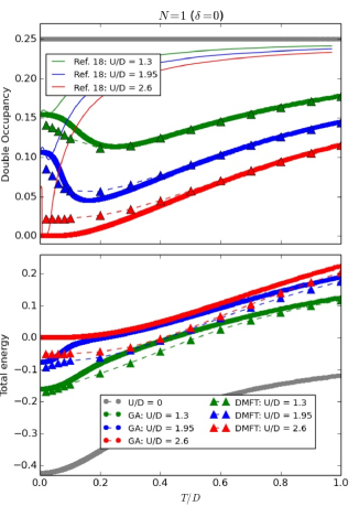
Figure 1: GA calculations of the single-band Hubbard model at half-filling ($N=1$) in comparison with DMFT+CTQMC and the data of Ref. Wang et al., 2010b. Upper panel: evolution of the double occupancy as a function of the temperature. Lower panel: evolution of the total energy as a function of the temperature.

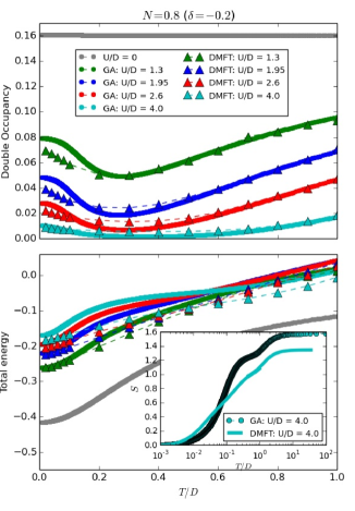
Figure 2: GA calculations of the single-band Hubbard model away from half-filling ($N=0.8$) in comparison with DMFT+CTQMC. Upper panel: temperature dependence of the double occupancy. Lower panel: temperature dependence of the total energy $\mathcal{E}(T)$. Inset of the lower panel: temperature dependence (in logaritmic scale) of the GA entropy $S$ in comparison with the DMFT data of Ref. Deng et al., 2013.

Numerical results.— Let us now discuss our numerical calculations of the Hubbard model, see Eq. (8). We assume a semicircular density of states (corresponding to a Bethe lattice in infinite dimensions)  and set the half-bandwidth $D$ as the unit of energy. For comparison, we perform DMFT calculations using the continuous time quantum Monte Carlo method with hybridization expansion Werner et al. (2006) as impurity solver, as implemented in TRIQS. Parcollet et al. (2015)

In the upper panel of Fig. 1 is shown the evolution of the double occupancy $d\equiv\langle c^{\dagger}_{R\uparrow}c^{\phantom{\dagger}}_{R\uparrow}c^{\dagger}_{R\downarrow}c^{\phantom{\dagger}}_{R\downarrow}\rangle$ as a function of the temperature at half-filling for several values of $U$. In the lower panel is shown the corresponding evolution of the total energy $\mathcal{E}$. The GA results are shown in comparison with DMFT and the Gutzwiller data of Ref. Wang et al., 2010b.

The agreement between the GA and DMFT+CTQMC is quantitatively satisfying, especially for smaller values of $U$ and higher temperatures (i.e., when the system is less correlated). Indeed, our method improves substantially the results obtained within the approximation scheme of Ref. Wang et al., 2010b. The slight quantitative discrepancy for larger $U$’s reflects the known fact that the Mott insulator is not well described by the GA, but is approximated by the simple atomic limit — that is a state with $d=0$. However, as long as the system is metallic, our extension of the GA to finite temperatures is remarkably accurate.

Let us now consider the Hubbard model away from half-filling. In particular, we consider the case of $N=0.8$ electrons per site (i.e., $\delta=-0.2$). In the upper panel of Fig. 2 is shown the temperature dependence of the double occupancy for several values of $U$, while in the lower panel is shown the evolution of the total energy $\mathcal{E}$. Finally, in the inset of the lower panel is shown the temperature dependence of the entropy for $U/D=4$, in comparison with the DMFT entropy calculated in Ref. Deng et al., 2013.

We point out that, as discussed before, the entropy is not evaluated directly from the GA variational parameters (which could be done only approximately, e.g., by using the entropy inequality of Ref. Sandri et al., 2013), but is calculated from the imaginary-time evolution of the total energy using the well known thermodynamical identities $dS=d\mathcal{E}/T$, $S(T=0)=0$. Note that the value of $S$ at $T\rightarrow\infty$ calculated according to these equations depends on the evolution of the total energy within the whole range of temperatures. It is for this reason that the GA entropy shown in Fig. 2 is slightly shifted with respect to DMFT at high temperatures — even though the atomic limit belongs to the GA variational space, and is thus captured exactly by our approximation scheme. 

The agreement between the GA and DMFT+CTQMC is even better for $N=0.8$ than for half-filling (which is to be expected, as the doped system is metallic for all $U$’s). In particular, it is remarkable that the agreement for $S$ is satisfying for $U/D=4$, which is the largest interaction strength considered.

In conclusion, we have developed an extension of the Gutzwiller approximation to finite temperatures based on the Dirac-Frenkel variational principle. Since our method does not rely on any entropy inequality, but only on the variational principle and the Gutzwiller approximation, it is as accurate as the ordinary GA theory for the ground state, and improves substantially the method previously proposed in Refs. Wang et al., 2010b; Sandri et al., 2013. We have performed benchmark calculations of the single-band Hubbard model at different fillings, and compared our results with DMFT+CTQMC, finding good quantitative agreement between the two methods in the metallic phase. We believe that our method will enable us to calculate from first principles several important physical quantities — such as the specific heat, the entropy and the temperature dependent structural properties — of strongly correlated systems presently too complex to be studied with more accurate methods, such as DMFT.