Recent measurements of the gravitational constant as a function of time

Abstract

A recent publication (J.D. Anderson et. al., EPL 110, 1002) presented a strong correlation between the measured values of the gravitational constant $G$ and the 5.9 year oscillation of the length of day. Here, we compile published measurements of $G$ of the last 35 years. A least squares regression to a sinusoid with period 5.9 years still yields a better fit than a straight line. However, our additions and corrections to the G data reported by Anderson et al. significantly weaken the correlation.

I Introduction

A recent article Anderson15 suggests a correlation between measurements of the gravitational constant, $G$, and the length of day. Figure 1 in Anderson15 shows 13 measurements of $G$ as a function of time. Superimposed is a sinusoidal fit with an offset of $\bar{G}=6.673\,90\,\times 10^{-11}\,{\mbox{m}}^{3}\,\mbox{kg}^{-1}\,\mbox{s}^{-2}$, a period $T=5.9$ years and amplitude $A=0.0016\,\times 10^{-11}\,{\mbox{m}}^{3}\,\mbox{kg}^{-1}\,\mbox{s}^{-2}$. The ratio of amplitude to offset is $2.43\times 10^{-4}$. A second trace shows a scaled version of the change in the length of day, almost indistinguishable from the fit, suggesting a strong correlation of $G$ measurements around the world and the observed change in the length of day.

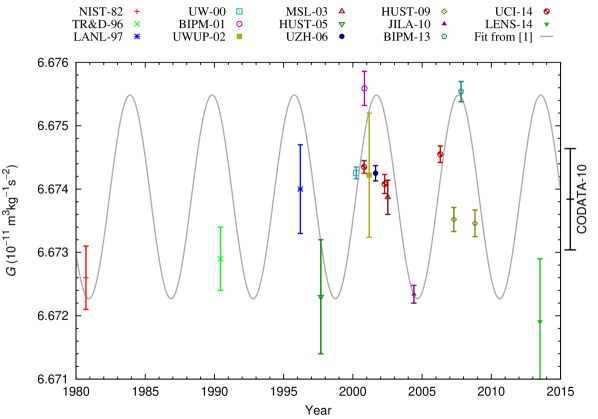
Figure 1: Measurements of the gravitational constant, $G$, as a function of time. The TR&D-96 data were taken over ten years; for this plot the final TR&D-96 result is shown at the average of their measurement dates. The solid gray sinusoidal curve is the fit to the data as it appears in Anderson15 ; it is indistinguishable from the scaled length-of-day-variation in the same reference. The point outside the frame gives the 2010 recommended value of $G$ with 1-sigma uncertainties according to the Task Group on Fundamental Constants of CODATA CODATA10 .

However, several points in [1] are not plotted at the right time and one experiment  Newman14 is missing. Here, we provide updated measured values of $G$ with their measurement dates, as displayed in Fig 1.

II Data sources

It is sometimes difficult to determine the exact time of data acquisition of a published $G$ measurement. Below we attempt to assign a best weighted average of the measurement times involved in each of the most precise $G$ measurements in the last 35 years. In some cases, this date is the mean of start and end date of the data acquisition period, in others, it is an average of individual dates when data was taken. This may not always be the best measure of the effective measurement time; in fitting data we suggest assigning an uncertainty for each tabulated time equal to 20 % of the time span.

NIST-82: This experiment was performed at the National Institute of Standards and Technology (then the National Bureau of Standards) in Gaithersburg, Maryland. A torsion balance used the so-called time-of-swing method in which torsional period is measured in at least two source mass configurations. $G$ is calculated from the difference in the squares of the periods and known mass distributions. The resulting $G=(6.672\,6\pm 0.000\,5)\times 10^{-11}\,{\mbox{m}}^{3}\,\mbox{kg}^{-1}\,\mbox{s}^{-2}$, was published in 1982 Luther82 . The measurement dates can be inferred from Table 1 in Luther80 . The first measurement was August 29 and the last October 10 1980. We use the average value, September 19 1980, as the time coordinate for this measurement.

TR&D-96: This measurement, performed in Moscow by researchers at Tribotech Research and Development Company, also used a torsion balance in the time-of-swing mode, yielding $G=(6.672\,9\pm 0.000\,5)\times 10^{-11}\,{\mbox{m}}^{3}\,\mbox{kg}^{-1}\,\mbox{s}^{-2}$, published in Karagioz96 . The results of measurements spanning 10 years are given in Table 3 of Karagioz96 . Unfortunately the data is given to only four decimal places. We reproduce the raw data with type A uncertainties in Table 1.

The TR&D-96 data alone permits a powerful test for a dependence of $G$ on length of day. Figure 2 shows the data (again with only type A uncertainties) as a function of time. The best fit to a sinusoid with period 5.9 years yields an offset $\bar{G}=6.672\,93\,\times 10^{-11}\,{\mbox{m}}^{3}\,\mbox{kg}^{-1}\,\mbox{s}^{-2}$ and amplitude of $A=0.000\,086\,\times 10^{-11}\,{\mbox{m}}^{3}\,\mbox{kg}^{-1}\,\mbox{s}^{-2}$ with uncertainty $\sigma_{A}=0.000\,055\,\times 10^{-11}\,{\mbox{m}}^{3}\,\mbox{kg}^{-1}\,\mbox{s}^{-2}$. There are 23 degrees of freedom and the $\chi^{2}$ is 14.3. Compared to the fit to a full $G$ data set in Anderson15 , this fit yields an amplitude smaller by a factor of 19 and phase differing by about 125 degrees.

In 2009, analysis of various correlations of the TR&D measurements to solar activity and other cosmic periods was published Parkhomov09 . Correlations were found, but were attributed to terrestrial effects — most probably variations in temperature and the microseismic environment. In Parkhomov09 data are shown ranging from 1985 to 2003. Unfortunately the data from 1995 to 2003 is not available to us.

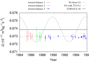
Figure 2: Data from Karagioz96 . Karagioz and Izmailov measured over a decade using three different torsion balances. Plotted uncertainties are type-A only. According to Ref. Karagioz96 the type B uncertainty associated with this experiment is $0.000\,52\times 10^{-11}\,{\mbox{m}}^{3}\,\mbox{kg}^{-1}\,\mbox{s}^{-2}$.

Date		$G\times 10^{11}$	$\sigma_{G}\times 10^{11}$
mm/dd/yyyy		$\left({\mbox{m}}^{3}\,\mbox{kg}^{-1}\,\mbox{s}^{-2}\right)$	$\left({\mbox{m}}^{3}\,\mbox{kg}^{-1}\,\mbox{s}^{-2}\right)$
04/19/1985		6.673 0	0.000 60
06/29/1985		6.673 0	0.000 43
12/11/1985		6.673 0	0.000 43
03/25/1986		6.673 0	0.000 29
01/04/1987		6.673 2	0.000 93
03/03/1987		6.672 9	0.000 30
07/14/1987		6.672 9	0.000 60
07/22/1987		6.673 0	0.000 17
09/24/1987		6.672 9	0.000 51
11/11/1987		6.672 9	0.000 30
08/02/1988		6.672 7	0.000 35
08/05/1988		6.672 9	0.000 18
03/09/1989		6.673 0	0.000 15
06/06/1989		6.672 9	0.000 22
06/20/1989		6.672 7	0.000 19
11/13/1990		6.673 0	0.000 09
03/21/1993		6.673 0	0.000 13
06/22/1993		6.672 9	0.000 34
11/30/1993		6.672 9	0.000 17
07/05/1994		6.672 8	0.000 06
12/20/1994		6.672 9	0.000 09
02/06/1995		6.672 9	0.000 13
05/25/1995		6.673 0	0.000 08
06/14/1995		6.673 0	0.000 38
08/24/1995		6.673 0	0.000 17
10/19/1995		6.672 7	0.000 07

Table 1: Measurements and type A uncertainties from Table 3 of Ref. Karagioz96 , with uncertainties converted to absolute values.

The TR&D-96 data can be averaged to yield a single data point as displayed in Fig. 1. The average of the dates listed in table 1 is June 9th 1990.

LANL-97: A time-of-swing experiment was performed at the Los Alamos National Laboratory in Los Alamos, New Mexico, yielding $G=(6.674\,0\pm 0.000\,7)\times 10^{-11}\,{\mbox{m}}^{3}\,\mbox{kg}^{-1}\,\mbox{s}^{-2}$  Bagley97 . The article gives no indication of when the data were taken. The thesis of C.H. Bagley Bagley97a gives some information. Written on page 15 is “In January of 1996, I attempted a trial Heyl-type determination with this arrangement, hoping for a percent number or better”. Later it is described how this measurement was much more precise, yielding the final value. On page 71 the reader learns that certain disturbances in the experiment became more frequent as the ambient temperature rose in April and May, until the data became unusable. The thesis was signed July 8 1996. Thus we take March 15 1996 as a time stamp for this data point.

UW-00: The measurement with the smallest uncertainty to date was performed at the University of Washington in Seattle, Washington, published in 2000 Gundlach00 . The rotation rate of a turntable supporting a torsion balance was varied such that the torsion fiber did not twist. In this angular-acceleration-feedback-mode the gravitational acceleration of a torsion pendulum towards source masses is fed back to the turntable, leaving the torsion balance motionless with respect to the turntable and adding the gravitational acceleration to the turntable motion. The gravitational constant is inferred from the second time derivative of the angle readout of the turntable with respect to time. The value published in 2000 must be slightly corrected due to an originally unconsidered effect of a small mass at the top of the torsion fiber which was also subject to the angular acceleration. This correction is described in CODATA02 . After correction, the final result is $G=(6.674\,255\pm 0.000\,092)\times 10^{-11}\,{\mbox{m}}^{3}\,\mbox{kg}^{-1}\,\mbox{s}^{-2}$. The times are documented in CODATA02 . Two sets of data were taken, one March 10 2000 to April 1 2000, the other April 3 2000 to April 18 2000. We use March 29 2000 to locate this $G$ value.

BIPM-01: These measurements used the first torsion pendulum built at the Bureau International des Poids et Mesures (BIPM) located in Sèvres, near Paris. The experiment measured $G$ with the same instrument operating with two methods. In the Cavendish method, the excursion of a torsion pendulum is measured for two source mass positions. The corresponding torques are obtained using a torsion constant determined from the balance s angular moment of inertia and free angular frequency.

In the electrostatic servo method, gravitational torque on the pendulum is compensated by an electrostatic torque produced by an electric potential applied to a capacitor with one plate on the pendulum bob and the other fixed. In this phase, the applied voltage is measured. A calibration experiment measured the capacitance as a function of pendulum angle. Combining the results of both methods yielded $G=(6.675\,59\pm 0.000\,27)\times 10^{-11}\,{\mbox{m}}^{3}\,\mbox{kg}^{-1}\,\mbox{s}^{-2}$  Quinn01 . The results of the Cavendish mode and servo mode are in close agreement, with $G=(6.675\,65\pm 0.000\,45)\times 10^{-11}\,{\mbox{m}}^{3}\,\mbox{kg}^{-1}\,\mbox{s}^{-2}$ from the Cavendish mode and $G=(6.675\,53\pm 0.000\,40)\times 10^{-11}\,{\mbox{m}}^{3}\,\mbox{kg}^{-1}\,\mbox{s}^{-2}$ from the servo mode. According to the authors Quinn15 , the servo data were obtained from September 29 to November 2 2000 and the Cavendish data from November 25 to December 13 2000. We take the effective date for the combined $G$ to be the average of the above dates.

UWUP-02: This experiment was located at the University of Wuppertal in Germany. The separation of two simple pendulums was measured with microwave interferometry. The forces on the pendulums and, hence, their separation was modulated by external moving source masses. The final value of this measurement, $G=(6.674\,22\pm 0.000\,98)\times 10^{-11}\,{\mbox{m}}^{3}\,\mbox{kg}^{-1}\,\mbox{s}^{-2}$ is published in a PhD thesis Kleinevoss02 . The appendix lists the data sets used for the final value. The first data set started January 12 2001, the last ended June 29 2001. Twelve data sets ranging in duration from 1 to 6 days were taken, mostly within a week of each other. A longer break occurred between March 7 and May 11 and between May 18 and June 25. Averaging the dates of the sets yields March 6.

MSL-03: This measurement, performed at the Measurement Standards Laboratory (MSL) of New Zealand, is the only recent measurement performed in the southern hemisphere. It employs a torsion balance in electrostatic servo mode with one difference: The calibration of the capacitance gradient is performed in an angular-acceleration experiment. The final value is $G=(6.673\,87\pm 0.000\,27)\times 10^{-11}\,{\mbox{m}}^{3}\,\mbox{kg}^{-1}\,\mbox{s}^{-2}$  Armstrong03 . One author Armstrong15 informed us that the data was gathered between March 21 2002 and November 1 2002. The average of these dates is July 11 2002.

HUST-05: This is the first measurement of $G$ performed at the Huazhong University of Science and Technology in Wuhan, China. A torsion balance in time-of-swing mode was used. A $G$ value published in 1999 Luo99 was subsequently corrected in 2005 for two small errors in mass distribution, yielding $G=(6.672\,3\pm 0.000\,9)\times 10^{-11}\,{\mbox{m}}^{3}\,\mbox{kg}^{-1}\,\mbox{s}^{-2}$. Data dates without years are given in the 1999 publication: seven sets of measurements were taken, the first starting on August 4 and the last ending on October 15. The authors report  Lu15 that the year was 1997.

We associate September 9 1997, equidistant in time from the start and end of the sets, with the HUST-05 $G$ measurement.

UZH-06: The experiment, performed by researchers at the University of Zürich, was located at the Paul Scherrer Institute near Villigen Switzerland. The gravitational force of a large mercury mass on two copper cylinders was measured with a modified commercial mass comparator, yielding $G=(6.674\,252\pm 0.000\,12)\times 10^{-11}\,{\mbox{m}}^{3}\,\mbox{kg}^{-1}\,\mbox{s}^{-2}$, published in 2006 Schlamminger06 . Figure 8 in this publication shows 43 days of data beginning July 31 2001 and ending September 9 and including a 6 day break. We take August 21 2001, as the effective date of this $G$ measurement.

HUST-09: A second torsion pendulum apparatus was constructed at HUST and used in time-of-swing mode to make two separate $G$ measurements, whose averaged value $G=(6.673\,49\pm 0.000\,18)\times 10^{-11}\,{\mbox{m}}^{3}\,\mbox{kg}^{-1}\,\mbox{s}^{-2}$ was first published in 2009 Luo09 . A long article on the same measurements was published in 2010 Tu10 , including the dates of the data sets used in the two experiments. The first experiment consisted of ten sets taken between March 21 2007 and May 20 2007. The second experiment started on October 8 2008 and ended on November 16 2008. The results for the first and second experiments are $G=(6.673\,52\pm 0.000\,19)\times 10^{-11}\,{\mbox{m}}^{3}\,\mbox{kg}^{-1}\,\mbox{s}^{-2}$ and $G=(6.673\,46\pm 0.000\,21)\times 10^{-11}\,{\mbox{m}}^{3}\,\mbox{kg}^{-1}\,\mbox{s}^{-2}$, respectively. Averaging the start and end dates of the sets, we obtain April 20 2007 and October 27 2008, respectively.

JILA-10: This experiment was performed at the Joint Institute for Laboratory Astrophysics in Boulder, Colorado. Similar to UWUP-02, two simple pendulums with separation determined by a laser interferometer were used to measure $G$, yielding $G=(6.672\,34\pm 0.000\,14)\times 10^{-11}\,{\mbox{m}}^{3}\,\mbox{kg}^{-1}\,\mbox{s}^{-2}$, reported in 2010  Parks10 . Figure 2 in this report and a table in  Parks14 show obtained values of $G$ as a function of time. Thirteen $G$ values were obtained in a time range May 12 to June 6 2004. Averaging the 13 dates yields May 28 2004.

Identifier	$G\times 10^{11}$	$\sigma_{G}\times 10^{11}$	Data acquisition			$e-s$	Device	Mode
	$\left({\mbox{m}}^{3}\,\mbox{kg}^{-1}\,\mbox{s}^{-2}\right)$	$\left({\mbox{m}}^{3}\,\mbox{kg}^{-1}\,\mbox{s}^{-2}\right)$	Start	End	Average	(Days)
NIST-82	$6.672\,6$	$0.000\,5$	08/29/1980	10/10/1980	09/19/1980	42	torsion balance	time-of-swing
TR&D-96	$6.672\,9$	$0.000\,5$	04/19/1985	10/19/1995	06/09/1990	3835	torsion balance	time-of-swing
LANL-97	$6.674\,0$	$0.000\,7$	01/01/1996	05/31/1996	03/15/1996	151	torsion balance	time-of-swing
UW-00	$6.674\,255$	$0.000\,092$	03/10/2000	04/18/2000	03/29/2000	39	torsion balance	acceleration servo
BIPM-01s	$6.675\,53$	$0.000\,40$	09/29/2000	11/02/2000	10/16/2000	34	torsion balance	electrostatic servo
BIPM-01c	$6.675\,65$	$0.000\,45$	11/25/2000	12/13/2000	12/04/2000	18	torsion balance	Cavendish
BIPM-01sc	$6.675\,59$	$0.000\,27$	09/29/2000	12/13/2000	11/02/2000	75	torsion balance	Cavendish & servo
UWUP-02	$6.674\,22$	$0.000\,98$	01/12/2001	06/29/2001	03/06/2001	168	two pendulums
MSL-03	$6.673\,87$	$0.000\,27$	03/21/2002	11/01/2002	07/11/2002	225	torsion balance	electrostatic servo
HUST-05	$6.672\,3$	$0.000\,9$	08/04/1997	10/15/1997	09/09/1997	72	torsion balance	time-of-swing
UZH-06	$6.674\,25$	$0.000\,12$	07/31/2001	08/21/2001	08/21/2001	21	beam balance
HUST-09a	$6.673\,52$	$0.000\,19$	03/21/2007	05/20/2007	04/20/2007	60	torsion balance	time-of-swing
HUST-09b	$6.673\,46$	$0.000\,21$	10/08/2008	11/16/2008	10/27/2008	39	torsion balance	time-of-swing
JILA-10	$\rule{20.00003pt}{0.0pt}6.672\,34$	$0.000\,14$	05/12/2004	06/06/2004	05/28/2004	25	two pendulums
BIPM-13s	$\rule{20.00003pt}{0.0pt}6.675\,15$	$0.000\,41$	11/08/2007	01/16/2008	12/15/2007	69	torsion balance	electrostatic servo
BIPM-13c	$\rule{20.00003pt}{0.0pt}6.675\,86$	$0.000\,36$	08/31/2007	09/10/2007	09/05/2007	10	torsion balance	Cavendish
BIPM-13sc	$\rule{20.00003pt}{0.0pt}6.675\,54$	$0.000\,16$	08/31/2007	01/16/2008	10/25/2007	138	torsion balance	Cavendish & servo
UCI-14a	$\rule{20.00003pt}{0.0pt}6.674\,35$	$0.000\,10$	10/04/2000	11/11/2000	10/23/2000	38	torsion balance	time-of-swing
UCI-14b	$\rule{20.00003pt}{0.0pt}6.674\,08$	$0.000\,15$	03/25/2002	05/12/2002	04/18/2002	48	torsion balance	time-of-swing
UCI-14c	$\rule{20.00003pt}{0.0pt}6.674\,55$	$0.000\,13$	04/08/2006	05/14/2006	04/26/2006	36	torsion balance	time-of-swing
LENS-14	$\rule{20.00003pt}{0.0pt}6.671\,91$	$0.000\,99$	07/05/2013	07/12/2013	07/08/2013	7	atom interferometer

Table 2: Summary of the most precise measurements of $G$ carried out in the last 35 years. The “Start” and “End” columns indicate our best estimate of the dates when data acquisition began and ended. The “Average” column shows our best estimate for the mean date of data acquisition. The “$e-s$” column gives the difference in days between end and start of data acquisition, important in estimating the amount by which a short-period signal is attenuated. We suggest 20 % of the $e-s$ duration number as a meaningful estimate of date uncertainty. We separate the two BIPM measurements into four measurements to emphasize that two different methods were used, and include data labeled BIPM-01sc and BIPM-13sc for the best $G$ and dates combining the two methods. Particularly for the 2013 BIPM data, results with the separate methods had strongly anti-correlated uncertainties, so that a $G(t)$ fit using the combined $G$ value can give a significantly different result from a fit treating results from the two methods separately. The BIPM data points in Figure 1 represent the combined $G$ data BIPM-01sc and BIPM-13sc.

BIPM-13: At the BIPM, a second torsion balance was constructed to measure $G$ with two different methods. Results were published in 2013 Quinn13 . Combining the results of both methods yielded $G=(6.675\,54\pm 0.000\,16)\times 10^{-11}\,{\mbox{m}}^{3}\,\mbox{kg}^{-1}\,\mbox{s}^{-2}$. The Cavendish and servo methods yielded $G=(6.675\,86\pm 0.000\,36)\times 10^{-11}\,{\mbox{m}}^{3}\,\mbox{kg}^{-1}\,\mbox{s}^{-2}$ and $G=(6.675\,15\pm 0.000\,41)\times 10^{-11}\,{\mbox{m}}^{3}\,\mbox{kg}^{-1}\,\mbox{s}^{-2}$, respectively. These numbers include a small correction published in an erratum in 2014 Quinn13 . Per one of the authors Quinn15 , the Cavendish data were obtained from August 31 to September 10 2007 and the servo mode data were measured in two campaigns, with November 8, 13, 14, and 16 in 2007 for the first campaign and January 11, 12, 13, 15, and 16 in 2008 for the second campaign. Averaging these dates we obtain October 25 2007 as an effective time stamp for the BIPM-13 data.

UCI-14: These measurements, performed using a torsion balance at cryogenic temperatures in time-of-swing mode, were made near Hanford, Washington. Three types of fibers with differing mechanical properties, especially amplitude dependence of the mechanical losses, were used. A result for each fiber was published in 2014 Newman14 : $G=(6.674\,35\pm 0.000\,10)\times 10^{-11}\,{\mbox{m}}^{3}\,\mbox{kg}^{-1}\,\mbox{s}^{-2}$, $G=(6.674\,08\pm 0.000\,15)\times 10^{-11}\,{\mbox{m}}^{3}\,\mbox{kg}^{-1}\,\mbox{s}^{-2}$, and $G=(6.674\,55\pm 0.000\,13)\times 10^{-11}\,{\mbox{m}}^{3}\,\mbox{kg}^{-1}\,\mbox{s}^{-2}$. The principal investigator provided the following time information: Data with the first fiber was first were obtained from October 4 2000 to November 11 2000. The average of these dates is October 23 2000. Data with the second fiber were obtained during two disjoint intervals. About 14 % of the data were obtained between December 8 and December 14 2000, The remainder between March 25 and May 12 2002. For simplicity we assign the average of the dates in 2002, i.e, April 18 2002 to the result with the second fiber. The true average of all dates for this fiber would be roughly January 30 2002. Measurements with the third fiber were collected from April 8 to May 15 2006. The mean of this interval is April 26 2006.

LENS-14: Following pioneering work at Stanford University Kasevich91 , a precision measurement of $G$ using a vertical atom interferometer was performed at the University of Florence, Italy. The phase shift between two paths is measured with two source mass configurations. The $G$ determined from the known mass distributions and the difference of the two phase, is $G=(6.671\,91\pm 0.000\,99)\times 10^{-11}\,{\mbox{m}}^{3}\,\mbox{kg}^{-1}\,\mbox{s}^{-2}$, published in 2014 Rosi14 . A longer account of the experiment appears in Prevedelli14 , which states that data was taken between July 5 and July 12 2013. The average of start and end date is July 8 2013. The experiment is on-going targeting an improved measurement of $G$.

In Table 2 we summarize the precision measurements of big G in the last 35 years.

II.1 Discussion

The main purpose of this article is to provide an as complete as possible list of $G$ values determined since 1980, while attempting to assign an as accurate as possible effective date for each measurement, providing data for further investigations similar to that of Anderson and collaborators.

Fit function	$T$	$A\times 10^{15}$		$\bar{G}\times 10^{11}$	Maximum	$\chi_{f}^{2}$	NDF	$P(\chi^{2}\geq\chi^{2}_{f})$	Remarks
	(years)	$\left({\mbox{m}}^{3}\,\mbox{kg}^{-1}\,\mbox{s}^{-2}\right)$		$\left({\mbox{m}}^{3}\,\mbox{kg}^{-1}\,\mbox{s}^{-2}\right)$
from Fig. 1 in [1]	5.93	16.1		6.673 88	09/13/01	381	14	$10^{-72}\rule{10.00002pt}{0.0pt}$
sine, fixed $T$	5.93	10.7		6.673 59	03/14/01	132	14	$10^{-21}\rule{10.00002pt}{0.0pt}$
sine, $T$ free	0.77	11.2		6.673 58	02/21/00	77	13	$10^{-11}\rule{10.00002pt}{0.0pt}$	global $\chi^{2}$ minimum
sine, $T$ free	6.17	11.0		6.673 54	02/13/01	124	13	$10^{-19}\rule{10.00002pt}{0.0pt}$	local $\chi^{2}$ minimum
straight line	n.a.	n.a.		6.674 13	n.a.	335	16	$10^{-61}\rule{10.00002pt}{0.0pt}$

Table 3: Fits to the $G$ data. Here the L2-norm is used exclusively. The “Maximum” column gives the date of the first maximum after 01/01/2000. The “NDF” column shows fits degrees of freedom.

We caution users of these data that it is very possible that much or all of the apparent $G$ time variation simply reflects overlooked systematic error, with underestimated systematic uncertainty.

However, we have ventured to make the following fits to data presented in this article, using the combined numbers for the two BIPM experiments.

1. A sinusoidal function with the parameters found in reference [1].

2. A sinusoidal function with free amplitude and phase but period fixed at 5.9 years.

3. A sinusoidal function with free amplitude, phase and period.

4. A single time-independent parameter, $\bar{G}$.

Results of these fits are presented in Table 3. These fits ignored uncertainties in date. Including uncertainties in both coordinates did not significantly affect fit results.

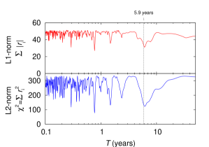
Figure 3: Goodness of fit as a function of period $T$. The upper graph shows the sum of the absolute residual: $\sum_{i}|r_{i}|$. The lower graph shows the sum of the squared residual: $\sum_{i}r_{i}^{2}$. The individual residual is given in both cases by $r_{i}=\left(G_{i}-\bar{G}-C\cos{(2\pi t_{i}/T)}-S\sin{(2\pi t_{i}/T)}\right)/\sigma_{i}$, where $G_{i}$ and $\sigma_{i}$ are determined at time $t_{i}$.

Figure 3 displays goodness of fit using two different norms for sinusoidal fits as $T$ is varied. The upper and lower graph show fits obtained by minimizing the sum of the absolute residual (L1-norm), $\sum_{i}|r_{i}|$, and the sum of the squared residual (L2-norm), $\sum_{i}r_{i}^{2}$, respectively. Here, $r_{i}$ is the residual of the i’th data point, given by $r_{i}=\left(G_{i}-\bar{G}-C\cos{(2\pi t_{i}/T)}-S\sin{(2\pi t_{i}/T)}\right)/\sigma_{i}$, where $G_{i}$ and $\sigma_{i}$ is the measurement and its uncertainty performed at time $t_{i}$. Fits using the L1-norm are less sensitive to outliers Barrodale68 . Of note in this plot are:

1. There are a number of local minima.

2. The lowest L1 and L2-norm are both located at $T=0.769$  years.

3. A local minimum is found at 6.1 years and 6.2 years for the L1- and L2-norm, respectively; not far from 5.9 years as found by Anderson et al..

4. There is a tantalizing local minimum in the L2-norm at 0.995 year.

We also made a least squares regression to the data taken over a period of more than ten years by Karagioz and Izmailov Karagioz96 , as discussed in the Data Sources section of this paper.

The situation is disturbing — clearly either some strange influence is affecting most $G$ measurements or, probably more likely, measurements of G since 1980 have unrecognized large systematic errors. The need for new measurements is clear.

Scientific exchange between groups measuring $G$ is necessary. The new working group on big $G$ under the auspices of International Union of Pure and Applied Physics (IUPAP) was formed to assist experimenters who are interested in these challenging measurements and wish to discuss and understand each other’s experiments.

II.2 Acknowledgment

We thank D.B. Newell and B.N. Taylor for assistance in locating some of the dates of the big $G$ experiments, and we thank the many G practitioners who provided us their best estimates of their measurement dates. We particularly thank J. Anderson and his collaborators for extremely helpful suggestions and data.

References

- (1) J.D. Anderson, G. Schubert, V. Trimble, and M.R. Feldman, EPL 110, 1002 (2015).
- (2) R. Newman, M. Bantel, E. Berg, and W. Cross, Phil. Trans. R. Soc. A 372, 20140025 (2014).
- (3) P.J. Mohr, B.N. Taylor, D.B. Newell, Rev. Mod. Phys. 84, 1527 (2010).
- (4) G.G. Luther and W.R. Towler, Phys. Rev. Lett. 48, 121 (1982).
- (5) G.G. Luther and W.R. Towler, in National Bureau of Standards Special Publication 617, Precision Measurement and Fundamental Constants II (1984) pp. 573.
- (6) O.V. Karagioz, V.P. Izmailov, Measurement Techniques 39, 979 (1996).
- (7) A.G. Parkhomov, Gravitation and Cosmology 15, 174 (2009).
- (8) C.H. Bagley and G.G. Luther, Phys. Rev. Lett. 78, 3047 (1997).
- (9) C.H. Bagley “A Determination of the Newtonian Constant of GravitationUsing the Method of Heyl” Ph.D. Thesis, University of Colorado, Boulder, Colorado, USA (1996).
- (10) J.H. Gundlach, S.M. Merkowitz, Phys. Rev. Lett. 85, 2869 (2000).
- (11) P.J. Mohr and B.N. Taylor, Rev. Mod. Phys. 77, 1 (2005).
- (12) T.J. Quinn, C.C. Speake, S.J. Richman, R.S. Davis, and A. Picard, Phys. Rev. Lett. 87, 111101 (2001).
- (13) T.J. Quinn, private communication, 2015.
- (14) U. Kleinevoß “Bestimmung der Newtonschen Gravitationskonstanten ”. Ph.D. Thesis, University of Wuppertal, Wuppertal, Germany.
- (15) T.R. Armstrong and M.P. Fitzgerald, Phys. Rev. Lett. 91 201101 (2003).
- (16) T.R. Armstrong, private communication, 2015.
- (17) J. Luo, Z.-K. Hu, X.-H. Fu,S.-H. Fan, and M.-X. Tang, Phys. Rev. D 59, 042001 (1998).
- (18) Z. Lu, private communication, 2015.
- (19) S. Schlamminger et al. Phys. Rev. D 74, 082001 (2006).
- (20) Z.-K. Hu, J.-Q. Guo, and J. Luo, Phys. Rev. D 71, 127505 (2005).
- (21) J. Luo, Q. Liu, L.-C. Tu, C.-G. Shao, L.-X. Liu, S.-Q. Yang, Q. Li, and Y.-T. Zhang, Phys. Rev. Lett. 102, 240801 (2009).
- (22) L.-C. Tu, Q. Li,Q.-L. Wang, C.-G. Shao, S.-Q. Yang, L.-X. Liu, Q. Liu, and J. Luo Phys. Rev. D 82, 022001 (2010).
- (23) H.V. Parks and J.E. Faller, Phys. Rev. Lett. 105, 110801 (2010).
- (24) H.V. Parks and J.E. Faller, Phil, Trans. R. Soc. A 372, 20140024 (2014).
- (25) T. Quinn, H. Parks, C. Speake, R. Davis, Phys. Rev. Lett. 111, 101102 (2013). Erratum. Phys. Rev. Lett. 113, 039901(E) (2014).
- (26) R. Newman et al., Phil, Trans. R. Soc. A 372 20140025 (2014).
- (27) M. Kasevich and S. Chu, Phys. Rev. Lett. 67, 181 (1991).
- (28) G. Rosi et al., Nature 510, 518 (2014).
- (29) M. Prevedelli et al., Phil, Trans. R. Soc. A 372, 20140030 (2014).
- (30) I. Barrodale, J. Roy. Stat. Soc. Ser. C Appl. Stat., 17 51 (1968).