Global diffeomorphism of the Lagrangian flow-map defining Equatorially trapped water waves

Abstract

The aim of this paper is to prove that a three dimensional Lagrangian flow which defines equatorially trapped water waves is dynamically possible. This is achieved by applying a mixture of analytical and topological methods to prove that the nonlinear exact solution to the geophysical governing equations, derived by Constantin in [5], is a global diffeomorphism from the Lagrangian labelling variables to the fluid domain beneath the free surface.

1 Introduction

In this paper we apply a mixture of analytical and topological methods to establish that a recently derived solution defining Equatorially trapped waves is dynamically possible. This remarkable solution, derived by Constantin in [5] and given below by equation (2.8), is an exact solution of the nonlinear $\beta-$plane governing equations for Equatorial water waves, and it is explicit in the Lagrangian framework. The main result of this paper establishes that the three-dimensional mapping (2.8) from the Lagrangian labelling domain to the fluid domain defines a global diffeomorphism— a consequence of which is that the solution (2.8) defines a fluid motion which is dynamically possible. We achieve this result by first establishing that (2.8) is locally diffeomorphic and injective, and then we render our results global by applying a suitable version of the classical degree-theoretic Invariance of Domain Theorem, cf. [10, 22].

The solution presented by Constantin in [5] represents a geophysical generalization of the celebrated Gerstner’s wave, in the sense that ignoring Coriolis terms in (2.8) recovers Gerstner’s wave solution. The primary importance of Gerstner’s wave is probably the fact that it represents the only known explicit and exact solution of the nonlinear periodic gravity wave problem with a non-flat free-surface. Gerstner’s wave is a two-dimensional wave propagating over a fluid domain of infinite depth (cf. [3, 4, 15]), and interestingly it may be modified to describe edge-waves propagating over a sloping bed [2, 26]. The geophysical solution presented in [5] encompasses Gerstner’s solution, yet it also possesses a number of inherent characteristics which transcends Gerstner’s wave. The solution (2.8) is a truly three-dimensional eastward-propagating geophysical wave, and furthermore it is Equatorially-trapped— achieving its greatest amplitude at the Equator and exhibiting a strong exponential decay in meridional directions away from the Equator. The solution is furthermore nonlinear, as is seen from the wave-surface profile, and has a dispersion relation that is dependant on the Coriolis parameter.

Since the solution (2.8) is explicit in the Lagrangian formulation, we may immediately discern some qualitative properties of the physical fluid motion. Indeed, an advantage of solutions in the Lagrangian framework is that the fluid kinematics may be explicitly described [1]. From (2.8) we see that at each fixed latitude the solution prescribes individual fluid particles to move clockwise in a vertical plane. Each particle moves in a circle, with the diameter of the circles decreasing exponentially with depth. In [5] it was simply shown that the solution (2.8) is compatible with the governing equations of the $\beta-$plane approximation for Equatorial water waves (2.3)-(2.7).

The aim of this paper is to rigorously justify that the fluid motion defined by (2.8) is dynamically possible. This is achieved by establishing that the solution (2.8) defines a global diffeomorphism, thereby ensuring that it is indeed possible to have a three-dimensional motion of the whole fluid body where all the particles describe circles with a depth- dependant radius at fixed latitudes, and furthermore the particles never collide but instead they fill out the entire infinite region below the surface wave. In so doing we show that the fluid domain as a whole evolves in a manner which is consistent with the full governing equations. We note that subsequent to the derivation of Constantin’s solution, a wide range of geophysical generalizations and variations to [5] have been produced and analysed, for example [6, 7, 8, 14, 16, 17, 18, 19, 20, 21]. It is expected that the rigorous considerations of this paper are also applicable to these variants.

2 The Equatorially trapped wave solution

2.1 Governing equations

We consider geophysical waves in the Equatorial region, where we assume that the earth is a perfect sphere of radius $R=6378$ km. We are in a rotating framework, where the $x$-axis is facing horizontal due east (zonal direction), the $y$-axis is due north (meridional direction), and the $z$-axis is pointing vertically upwards. The governing equations for geophysical ocean waves are given by Euler’s equation with additional terms involving the Coriolis parameter which is proportional to the rotation speed of the earth, see [9, 23]

$$\left\{\begin{array}[]{ll}u_{t}+uu_{x}+vu_{y}+wu_{z}\,+2\Omega w\cos\Phi-2\Omega v\sin\Phi&\displaystyle=-{1\over\rho}P_{x}\vskip 3.0pt plus 1.0pt minus 1.0pt\\ v_{t}\,+uv_{x}\,+vv_{y}\,+wv_{z}\,+2\Omega u\sin\Phi&\displaystyle=-{1\over\rho}P_{y}\vskip 3.0pt plus 1.0pt minus 1.0pt\\ w_{t}+uw_{x}+vw_{y}+ww_{z}-2\Omega u\cos\Phi&\displaystyle=-{1\over\rho}P_{z}-g,\end{array}\right.$$ (2.1)

the mass conservation equation

$$\rho_{t}+u\rho_{x}+v\rho_{y}+w\rho_{z}=0$$ (2.2)

and the equation of incompressibility

$$u_{x}+v_{y}+w_{z}=0.$$ (2.3)

Here $\Phi$ represents the latitude, $(u,v,w)$ is the fluid velocity, $\Omega=73.10^{-6}$ rad$/$s is the (constant) rotational speed of earth (which is the sum of the rotation of the earth about its axis and the rotation around the sun, see [9]), $g=9.8$ m/s^-2 is the gravitational constant, $\rho$ is the water density, and $P$ is the pressure.

We are interested in Equatorial waves, that is, geophysical ocean waves in a region which is within $5^{o}$ latitude of the Equator. Since the latitude is small, we may use the approximations $\sin\Phi\approx\Phi$, and $\cos\Phi\approx 1$, and thus linearising the Coriolis force leads to the $\beta$-plane approximation to equations (2.1) given by

$$\left\{\begin{array}[]{ll}u_{t}+uu_{x}+vu_{y}+wu_{z}+2\Omega w-\beta yv&\displaystyle=-{1\over\rho}P_{x}\vskip 3.0pt plus 1.0pt minus 1.0pt\\ v_{t}+\,uv_{x}\,+vv_{y}+\,wv_{z}+\beta yu&\displaystyle=-{1\over\rho}P_{y}\vskip 3.0pt plus 1.0pt minus 1.0pt\\ w_{t}+uw_{x}+vw_{y}+ww_{z}-2\Omega u&\displaystyle=-{1\over\rho}P_{z}-g,\end{array}\right.$$ (2.4)

where $\beta=2\Omega/R=2.28\cdot 10^{-11}$ m^-1s^-1. The relevant boundary conditions are the kinematic boundary conditions

$$w=\eta_{t}+u\eta_{x}+v\eta_{y}\mbox{ on }z=\eta(x,y,t),$$ (2.5)

$$P=P_{atm}\mbox{ on }z=\eta(x,y,t),$$ (2.6)

where $P_{atm}$ is the (constant) atmospheric pressure, and $\eta(x,y,t)$ is the free surface. The boundary condition (2.5) states that all the particles in the surface will stay in the surface for all time $t$, and the boundary condition (2.6) decouples the water flow from the motion of the air above. We work with an infinitely-deep fluid domain and so we require the velocity field to converge rapidly to zero with depth, that is

$$(u,w)\to(0,0)\;\mbox{ as }\;z\to-\infty.$$ (2.7)

The governing equations for the $\beta-$plane approximation of geophysical ocean waves are given by (2.3)-(2.7).

2.2 Exact solution

In this section we present and describe briefly the exact solution of the $\beta$-plane governing equations (2.3)-(2.7) which was recently derived by Constantin [5]. This solution describes a three- dimensional eastward-propagating geophysical wave which is Equatorially trapped, exhibiting a strong exponential decay in meridional directions away from the Equator, and which is periodic in the zonal direction. Equatorially trapped waves propagating eastward and symmetric about the Equator are known to exist, and they are regarded as one of the key factors in a possible explanation of the El Niño phenomenon (cf. [9, 11]). The formulation of the solution employs a Lagrangian viewpoint, describing the evolution in time of an individual fluid particle [1]. The Lagrangian positions of the fluid $(x,y,z)$ are given in terms of the labelling variables $(q,r,s)$, and time $t$ by

$$\left\{\begin{array}[]{rl}x&\displaystyle=q-{1\over k}e^{k\left[r-f(s)\right]}\sin\left[k(q-ct)\right],\\ y&\displaystyle=s,\\ z&\displaystyle=r+{1\over k}e^{k\left[r-f(s)\right]}\cos\left[k(q-ct)\right],\end{array}\right.$$ (2.8)

where $k$ is the wave number, defined by $k=2\pi/L$ where $L$ is the wavelength, and the wave phase speed is determined by the dispersion relation

$$c={\sqrt{\Omega^{2}+kg}-\Omega\over k},$$ (2.9)

and also

$$f(s)={c\beta\over 2g}s^{2}$$ (2.10)

determines the decay of fluid particle oscillations in the meridional direction. The labelling variables take the values $(q,r,s)\in{\mathbb{R}}\times(-\infty,r_{0})\times{\mathbb{R}}$, where $r_{0}\leq 0$ is fixed. For every fixed $s$, the system (2.8) describes the flow beneath a surface wave propagating eastwards (in the $x$-direction) at constant speed $c$ determined by (2.9). At fixed latitudes (that is, for $s$ fixed) the free surface $z=\eta(x,y,t)$ is obtained by setting $r=r_{0}(s)$ in the third equation in (2.8), where $r_{0}(s)<r_{0}$ is the unique solution to

$${e^{2k\left[r_{0}(s)-f(s)\right]}\over 2k}-r_{0}(s)={e^{2kr_{0}}\over 2k}-r_{0}.$$

A plot of the free-surface for the wave solution (2.8) is given in Figure 1 below.

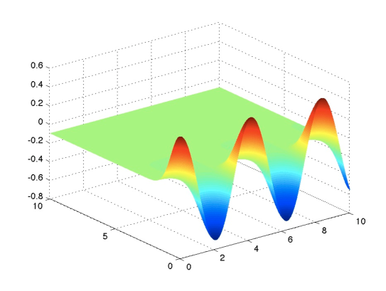
Figure 1: Exact solution (2.8).

In [5] the author focuses on proving, by explicit computation, that the exact solution (2.8) is compatible with the governing equations (2.3)-(2.7). Our aim in this work is to prove that it is dynamically possible to have a global motion of the fluid domain where, at fixed latitudes, the particles move in circular paths with depth-dependant radius. Indeed, we prove in our main result Proposition 3.3 that the fluid motion defined by (2.8) is dynamically possible, that is, at any instant $t$, the label map is a global diffeomorphism from the labelling variables, $\{(q,r,s):q\in{\mathbb{R}},\,r\leq r_{0}\mbox{ and }s\in{\mathbb{R}}\}$, to the fluid domain beneath the free surface given by

$$(q,s)\mapsto\left(q-{1\over k}e^{r_{0}(s)-f(s)}\sin\left[k(q-ct)\right],s,r_{0}(s)+{1\over k}e^{r_{0}(s)-f(s)}\cos\left[k(q-ct)\right]\right).$$ (2.11)

For a fixed latitude $s$, the surface wave profile (2.11) is a reverse trochoid if $r_{0}(s)<0$ and a reverse cycloid with a cusp at the wave crest if $r_{0}(s)=0$ and $s=0$.

Fixed $s$, and given $k>0$ and $r_{0}(s)\leq 0$, the curve $z=h_{s}(x)$ given parametrically by

$$\xi\mapsto\left({\xi\over k}-{e^{r_{0}(s)-f(s)}\over k}\sin\left(\xi\right),{1\over k}-{e^{r_{0}(s)-f(s)}\over k}\cos\left(\xi\right)\right)$$ (2.12)

is a trochoid if $r_{0}(s)-f(s)<0$ and a cycloid if $r_{0}(s)-f(s)=0$. It represents the curve traced by a fixed point at a distance ${e^{r_{0}(s)-f(s)}\over k}<{1\over k}$ from the center of a circle of radius ${1\over k}$ rolling along a straight line without slipping, (see Figure 2).

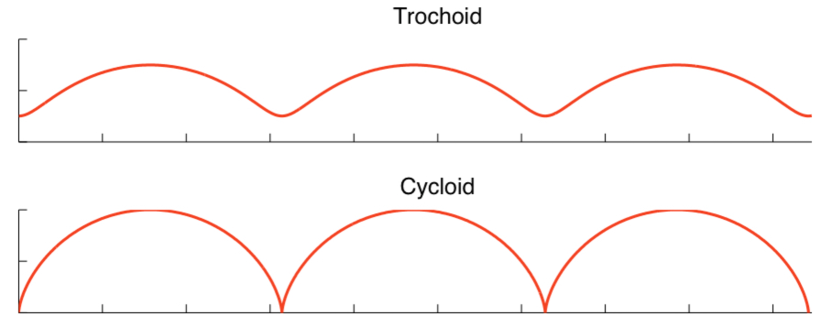
Figure 2: Trochoid and cycloid curves.

Therefore, for a fixed latitude $s$, the free surface of the fluid has the equation $z=r_{0}(s)+{1\over k}-h_{s}(x-ct)$ which represents a reverse trochoid propagating to the right with velocity $c$. Since $h_{s}$ is periodic with minimal period ${2\pi/k}$ then the surface is a periodic wave with period ${2\pi/k}$, which concurs with the definition of the wave number $k$.

3 Main results

To prove that the motion (2.8) is dynamically possible, it is sufficient to analyse (2.8) for the time $t=0$, when it takes the form

$$\left\{\begin{array}[]{rl}x&\displaystyle=q-{e^{k\left[r-f(s)\right]}\over k}\sin\left(kq\right),\\ y&=s\\ z&\displaystyle=r+{e^{k\left[r-f(s)\right]}\over k}\cos\left(kq\right).\end{array}\right.$$ (3.1)

The case of a general time $t$ in (2.8) is recovered making first the change of variables $(q,r,s)\mapsto(q+ct,r,s)$, performing (3.1), and finally shifting the horizontal variable $x$ by $ct$. Therefore we can focus on (3.1), and we further note that as $q$ varies by $2\pi/k$, the $z$ value reoccurs and $x$ is shifted linearly by $2\pi/k$. Hence, it suffices to analyse (3.1) on the domain

$$\mathcal{D}=\left\{(q,r,s):q\in\left[0,{2\pi\over k}\right],r\leq r_{0}\mbox{ and }s\in{\mathbb{R}}\right\}.$$

In the following result we first prove that the map (3.1) is an injective local diffeomorphism.

Lemma 3.1.

For every fixed $t\geq 0$, if $r_{0}<0$ then the map (3.1) is a local diffeomorphism from $\mathcal{D}=\left\{(q,r,s):q\in\left[0,{2\pi\over k}\right],r\leq r_{0}\mbox{ and }s\in{\mathbb{R}}\right\}$ into its image injectively. In the limiting case $r_{0}=0$, then this result holds for the domain $\mathcal{D}$ excluding the cusps at the equatorial wave-crests.

Proof.

We remark first that $r-f(s)\leq r_{0}-f(s)\leq r_{0}\leq 0$, as we see from the definition of $r_{0}$ and (2.10). The differential of (3.1) at a point $(q,r,s)$ is given by

$$\left(\begin{array}[]{ccc}1-e^{k(r-f(s))}\cos(kq)&f^{\prime}(s)e^{k(r-f(s))}\sin(kq)&-e^{k(r-f(s))}\sin(kq)\\ 0&1&0\\ -e^{k(r-f(s))}\sin(kq)&f^{\prime}(s)e^{k(r-f(s))}\cos(kq)&1+e^{k(r-f(s))}\cos(kq)\end{array}\right)$$ (3.2)

with determinant $1-e^{2k(r-f(s))}$. As an aside, we note that the time independence of this expression implies that the fluid is incompressible and so (2.3) holds, cf. [5]. It follows that if $r_{0}<0$ the Jacobian of (3.1) is non-zero (strictly positive) everywhere, whereas in the case $r_{0}=0$ the Jacobian is zero precisely at the Equator ($s=0$), where the break-down in regularity corresponds to the appearance of cusps at the wave-crest as discussed above. Therefore, aside from the situation when $r_{0}=s=0$, the mapping (3.1) is differentiable, continuous with non-zero derivative, and hence we can apply the Inverse Function Theorem to infer that (3.1) is a smooth local diffeomorphism onto its image.

Let us prove now that (3.1) is injective. Let $(q_{i},r_{i},s_{i})\in\mathcal{D}$ for $i=1,2$, and let $\big{(}x(q_{i},r_{i},s_{i}),y(q_{i},r_{i},s_{i}),z(q_{i},r_{i},s_{i})\big{)}$ be the corresponding fluid particles given by (3.1). First of all, if

$$\big{(}x(q_{1},r_{1},s_{1}),y(q_{1},r_{1},s_{1}),z(q_{1},r_{1},s_{1})\big{)}=\big{(}x(q_{2},r_{2},s_{2}),y(q_{2},r_{2},s_{2}),z(q_{2},r_{2},s_{2})\big{)}$$

then $s_{1}=s_{2}$. Thus, we can fix $s$ and then focus on checking injectivity with respect to $x$ and $z$ in (3.1). Letting $\xi=q+ir$, then the values of $(x,z)$ in (3.1) correspond to the map

$$\xi\mapsto\xi+i{e^{-kf(s)}\over k}e^{ik\overline{\xi}}.$$

To prove injectivity, we consider $F(\xi)=\xi+g(\xi)$, where $\xi=(q,r)$. Let $\xi_{1}\neq\xi_{2}$, then applying the Mean Value Theorem we derive

$$\begin{array}[]{ll}\left|F(\xi_{1})-F(\xi_{2})\right|&\displaystyle\geq\left|\xi_{1}-\xi_{2}\right|-\left|g(\xi_{1})-g(\xi_{2})\right|\vskip 3.0pt plus 1.0pt minus 1.0pt\\ &\displaystyle\geq\left|\xi_{1}-\xi_{2}\right|-\max\limits_{s\in[0,1]}\|Dg_{s\xi+(1-s)\xi_{2}}\|\left|\xi_{1}-\xi_{2}\right|.\end{array}$$ (3.3)

Computing $Dg$ in terms of $(q,r)$, yields

$$Dg_{(q,r)}=e^{k(r-f(s))}\left(\begin{array}[]{cc}-\cos(kq)&-\sin(kq)\\ -\sin(kq)&\cos(kq)\end{array}\right)$$ (3.4)

then $\|Dg_{(q,r)}\|=e^{2k(r-f(s))}$. From (3.3), and considering that $\xi_{i}=(q_{i},r_{i})$ for $i=1,2$, we obtain that

$$\begin{array}[]{ll}\left|F(\xi_{1})-F(\xi_{2})\right|&\displaystyle\geq\displaystyle\left|\xi_{1}-\xi_{2}\right|-e^{2k(\max\{r_{1},r_{2}\}-f(s))}\left|\xi_{1}-\xi_{2}\right|\\ &\displaystyle=\big{(}1-e^{2k(\tilde{r}-f(s))}\big{)}\left|\xi_{1}-\xi_{2}\right|,\end{array}$$

where $\tilde{r}=\max\{r_{1},r_{2}\}$. Therefore, if $\tilde{r}-f(s)<0$, $F$ is injective, and we have proved that (3.1) is injective. ∎

The following result will be used to prove that (2.8) is in fact a global diffeomorphism, cf. [22], [25].

Theorem 3.2.

(Invariance of Domain theorem) If $U\subset{\mathbb{R}}^{n}$ is open and $F:U\to{\mathbb{R}}^{n}$ is a continuous one-to-one mapping, then $F:U\to F(U)$ is a homeomorphism, and $F(\partial\overline{U})=\partial F(\overline{U})$.

We have already proved in Lemma 3.1 that the exact solution (3.1) gives us a local diffeomorphism that is globally injective on $\mathcal{D}$. The result below proves that (2.8) is a global diffeomorphism for all $t\geq 0$, this is, that (2.8) is dynamically possible.

Proposition 3.3.

For every fixed $t\geq 0$, if $r_{0}\leq 0$ the map (2.8) is a global diffeomorphism from $\mathcal{V}=\left\{(q,r,s):q\in{\mathbb{R}},r<r_{0}\mbox{ and }s\in{\mathbb{R}}\right\}$ into the fluid domain beneath the free surface $z=\eta(x,y,t)$. Moreover, if $r_{0}<0$ the free surface $z=\eta(x,y,t)$ has a smooth profile, and in the limiting case $r_{0}=0$ the free surface is piecewise smooth with upward cusps at $s=0$.

Proof.

From Lemma 3.1, we know that the map (3.1) is an injective local diffeomorphism from $\mathcal{D}=\left\{(q,r,s):q\in\left[0,{2\pi\over k}\right],r\leq r_{0}\mbox{ and }s\in{\mathbb{R}}\right\}$ into its image. To prove that the local diffeomorphism is in fact a global diffeomorphism we just have to prove that it is a homeomorphism. Indeed, since the hypotheses in the Invariance of Domain Theorem 3.2 are satisfied, then the map (3.1) is a homeomorphism. Although it is guaranteed by the Invariance Domain Theorem 3.2, we can see directly that the map (3.1) sends $\partial\overline{\mathcal{D}}$ into the boundaries of the image of $\overline{\mathcal{D}}$. The vertical semiplanes $\left\{(0,r,s):r\leq r_{0}\mbox{ and }s\in{\mathbb{R}}\right\}$ and $\left\{\!(2\pi/k,r,s):r\leq r_{0}\mbox{ and }s\in{\mathbb{R}}\right\}$ are transformed by (3.1) in the vertical surfaces $\left\{\!(0,y,z)\!:\!z\leq r_{0}(s)+{e^{k(r_{0}(s)-f(s))}\over k},\,y\in{\mathbb{R}}\right\}$ and $\left\{(2\pi/k,y,z)\!:\!z\leq r_{0}(s)+{e^{k(r_{0}(s)-f(s))}\over k},\,y\in{\mathbb{R}}\right\}$ respectively, and the horizontal semiplane $\left\{(q,r_{0},s):0\leq q\leq 2\pi/k\mbox{ and }s\in{\mathbb{R}}\right\}$ becomes part of the reverse trochoid if $r_{0}(s)-f(s)<0$, which is smooth, and it becomes part of the reverse cycloid if $r_{0}(s)=0$ and $s=0$, which is piecewise smooth with upward cusps.

We have proved that (3.1) is a global diffeomorphism map from $\mathcal{D}$ into its image if $r_{0}<0$, with singularities occurring when $r_{0}=0$ and $s=0$. Since the full system (2.8) can be recovered from (3.1) by making the change of variables $(q,r,s)\mapsto(q+ct,r,s)$, and finally shifting the horizontal variable $x$ by $ct$, it follows that (2.8) is a global diffeomorphism from $\mathcal{V}=\left\{(q,r,s):q\in{\mathbb{R}},r<r_{0}\mbox{ and }s\in{\mathbb{R}}\right\}$ into the fluid domain below the free surface. ∎

References

- [1] Bennett, A. Lagrangian fluid dynamics. Cambridge University Press, 2006.
- [2] Constantin, A. Edge waves along a sloping beach. J. Phys. A 34, 45 (2001), 9723–9731.
- [3] Constantin, A. On the deep water wave motion. J. Phys. A 34, 7 (2001), 1405–1417.
- [4] Constantin, A. Nonlinear water waves with applications to wave-current interactions and tsunamis, vol. 81. SIAM, 2011.
- [5] Constantin, A. An exact solution for equatorially trapped waves. J. Geophys. Res. 117 (2012), C05029.
- [6] Constantin, A. Some three-dimensional nonlinear Equatorial flows. J. Phys. Oceanogr. 43 (2013), 165–175.
- [7] Constantin, A. Some nonlinear, equatorially trapped, nonhydrostatic internal geophysical waves, J. Phys. Oceanogr. 44 (2014), 781–789.
- [8] Constantin, A. and Germain, P. Instability of some equatorially trapped waves. J. Geophys. Res. Oceans 118 (2013) 2802–2810.
- [9] Cushman-Roisin, B., and Beckers, J.-M. Introduction to geophysical fluid dynamics: physical and numerical aspects, vol. 101. Academic Press, 2011.
- [10] Deimling, K. Nonlinear functional analysis. Springer-Verlag, Berlin, 1985.
- [11] Fedorov, A. V., and Brown, J. N. Equatorial waves. In Encyclopedia of Ocean Sciences, J. Steele, Ed. Academic, San Diego, Calif., 2009, pp. 3679–3695.
- [12] Friedlander, S., and Serre, D., Eds. Handbook of mathematical fluid dynamics. Vol. IV. North-Holland, Amsterdam, 2004.
- [13] Gerstner, F. Theorie der Wellen samt einer daraus abgeleiteten Theorie der Deichprofile. Ann. Phys. 2 (1809), 412–445.
- [14] Genoud, F. and Henry, D. Instability of equatorial water waves with an underlying current. J. Math. Fluid Mech. 16 (2014), 661–667.
- [15] Henry, D. On Gerstner’s water wave. Journal of Nonlinear Mathematical Physics 15, sup2 (2008), 87–95.
- [16] Henry, D. An exact solution for equatorial geophysical water waves with an underlying current. Eur. J. Mech. B Fluids 38 (2013), 18–21.
- [17] Henry, D. and Hsu, H.-C. Instability of internal equatorial water waves. J. Differential Equations 258 (2015), 1015–1024.
- [18] Henry, D. and Hsu, H.-C. Instability of equatorial water waves in the plane, Discrete Contin. Dyn. Syst. 35 (2015), 909–916.
- [19] Ionescu-Kruse, D. An exact solution for geophysical edge waves in the plane approximation. Nonlinear Anal. Real World Appl. 24 (2015), 190–195.
- [20] Matioc, A. V. An exact solution for geophysical equatorial edge waves over a sloping beach. J. Phys. A 45 365501 (2012).
- [21] Matioc, A. V. Exact geophysical waves in stratified fluids. Appl. Anal. 92 (2013), 2254–2261.
- [22] Krawcewicz, W., and Wu, J. Theory of degrees with applications to bifurcations and differential equations. Canadian Mathematical Society Series of Monographs and Advanced Texts. John Wiley & Sons, Inc., New York, 1997. A Wiley-Interscience Publication.
- [23] Pedlosky, J. Geophysical Fluid Dynamics. Springer, 1992.
- [24] Rankine, W. J. M. On the exact form of waves near the surface of deep water. Philos. Trans. R. Soc. London A 153 (1863), 127–138.
- [25] Rothe, E. H. Introduction to various aspects of degree theory in Banach spaces, vol. 23 of Mathematical Surveys and Monographs. American Mathematical Society, Providence, RI, 1986.
- [26] Stuhlmeier, R. On edge waves in stratified water along a sloping beach. J. Nonlinear Math. Phys. 18 (2011), 127–137.