Diphoton production at Tevatron and the LHC in the NLO^⋆ approximation of the Parton Reggeization Approach.

Abstract

The hadroproduction of prompt isolated photon pairs at high energies is studied in the NLO^⋆ framework of the Parton Reggeization Approach. The real part of the NLO corrections is computed, and the procedure for the subtraction of double counting between real parton emissions in the hard-scattering matrix element and unintegrated PDF is constructed for the amplitudes with Reggeized quarks in the initial state. The matrix element of the important NNLO subprocess $RR\to\gamma\gamma$ with full dependence on the transverse momenta of the initial-state Reggeized gluons is obtained. We compare obtained numerical results with diphoton spectra measured at Tevatron and the LHC, and find a good agreement of our predictions with experimental data at the high values of diphoton transverse momentum, $p_{T}$, and especially at the $p_{T}$ larger than the diphoton invariant mass, $M$. In this multi-Regge kinematics region, the NLO correction is strongly suppressed, demonstrating the self consistency of the Parton Reggeization Approach.

I Introduction

Nowadays, the inclusive hadroproduction of pairs of isolated prompt photons (diphotons) is a subject of intense experimental and theoretical studies. From the experimental point of view, this process forms an irreducible background in the searches of heavy neutral resonances in the diphoton decay channel, such as Standard Model Higgs boson SM_Higgs_disc and it’s Beyond Standard Model counterparts BSM_anal . As for the process itself, it allows us to define the set of inclusive differential cross sections over such variables as the invariant mass of the pair ($M$), it’s transverse momentum ($p_{T}$), azimuthal angle between transverse momenta of the photons ($\Delta\phi$), rapidity of the photon pair ($Y_{\gamma\gamma}$), Collins-Soper angle in the center of mass frame of the photon pair ($\theta$) and a few others CDF_data_2012 . Most of these spectra are measured with high precision both at Tevatron CDF_data_2012 and the LHC ATLAS_data_2013 .

On the theoretical side, providing the predictions for the above mentioned rich set of differential spectra is a challenging task even for the state of the art techniques in perturbative Quantum Chromodynamics (pQCD). While, for the inclusive isolated prompt photon production, the $p_{T}$-spectra from CDF CDF_1gamma , ATLAS ATLAS_1gamma and CMS CMS_1gamma are described within experimental uncertainties in the Next to Leading Order (NLO) of conventional Collinear Parton Model (CPM) of the QCD Jetphox . Also, the notably good results where obtained for these spectra already in the Leading Order (LO) of $k_{T}$-factorization in the Ref. SVAphoton ; KSSY_photon_jet . In contrast, existing NLO CPM calculations, implemented in the DIPHOX Diphox Monte-Carlo event generator, provide very poor description of $p_{T}$ and $\Delta\phi$ distributions measured by ATLAS ATLAS_data_2013 . In the CPM, the full NNLO accuracy is required to provide qualitatively reasonable description of all distributions 2gNNLO .

Part of these difficulties can be traced back to the shortcomings of the CPM approximation, where the transverse momentum of initial state partons is integrated over in the Parton Distribution Functions (PDFs), but neglected in the hard scattering part of the process. Such treatment is justified for the fully inclusive single scale observables, such as deep inelastic scattering structure functions or $p_{T}$-spectra of single prompt photons and jets, where the corrections breaking the collinear factorization are shown to be suppressed by a powers of the hard scale Collins_QCD .

For the multi-scale differential observables, there is no obvious reason why the fixed-order calculation in the CPM should be a good approximation. Usually the simple picture of factorization of the cross section of the hard process into the convolution of hard-scattering coefficient and some PDF-like objects is kept, but kinematical approximations are relaxed. In the treatment of Initial State Radiation (ISR) corrections in the Soft Collinear Effective Theory (SCET) SCET or in the Transverse Momentum Dependent (TMD) factorization formalism TMD_Noevol ; CSS_resumm ; Collins_QCD , the transverse-momentum of the initial-state parton is kept unintegrated on the kinematical level, but neglected in the hard-scattering part, which is justified e. g. when the $p_{T}$ of the exclusive final state is much smaller than it’s invariant mass, so that the following hierarchy of the light-cone momentum components for the initial-state parton is preserved: $q^{\mp}\ll|{\bf q}_{T}|\ll q^{\pm}=x\sqrt{S}$.

In the opposite limit, when $q^{\mp}\ll|{\bf q}_{T}|\sim q^{\pm}=x\sqrt{S}$, the $k_{T}$-factorization kTf is valid, and transverse momentum of the initial state parton can no longer be neglected in the hard scattering amplitudes. To obtain the suitable hard scattering matrix element we will apply the hypothesis of parton Reggeization, which will be described below. In what follows we will refer to the combination of $k_{T}$-factorization with hard scattering matrix elements with Reggeized partons in the initial state as the Parton Reggeization Approach (PRA). This approach is mostly suitable for the study of the production of the final states with high $p_{T}$ and small invariant mass in the central rapidity region. At high energies $\sqrt{S}\gg p_{T}$, such final states are produced by the small-$x$ partons, and the resummation of $\log(1/x)$-enhanced terms into the unintegrated PDF (unPDF) can be implemented CCFM . Clearly, the regions of applicability of the TMD and $k_{T}$-factorization are overlapping, and they should match when $x\to 1$.

Turning back to the photon pair production, we can conclude, that neither TMD nor $k_{T}$-factorization covers all available range of experimental data. Most of the cross section comes from the region where the diphoton has small $p_{T}$ and photons fly nearly back-to-back in the transverse plane, so additional QCD radiation is kinematically constrained to be soft and collinear, and the approach of SCET factorization will be preferable. On the contrary, at high $p_{T}$ and small $\Delta\phi$, the $k_{T}$-factorization will do a good job, as we will show below.

The previous attempts to study the prompt diphoton production in $k_{T}$-factorization Saleev_gg ; A_Lipatov_gg had their own problems. In the Ref. Saleev_gg , only LO $2\to 2$ subprocesses where taken into account. While, the PRA was used to obtain the gauge invariant expression for the $Q\bar{Q}\to\gamma\gamma$ matrix element with off-shell initial state Reggeized quarks ($Q$), the matrix element for the $RR\to\gamma\gamma$ with off-shell Reggeized gluons in the initial state was taken the same as in the CPM. In fact, this contribution was overestimated in Ref. Saleev_gg due to the erroneous overall factor 4 in the partonic cross section of the subprocess $gg\to\gamma\gamma$ presented in the Ref. BergerBraatenField , which have lead to the accidental agreement with the early Tevatron data CDF_old . This factor was carefully checked against the results presented in the literature BoxCPM ; Bern_gg_gaga , as well as by our independent calculations of the exact $RR\to\gamma\gamma$ amplitude, described in the Sec. IV of the present paper.

In the Ref. A_Lipatov_gg , the attempt to take into account the NLO $2\to 3$ subprocesses was made, but manifestly non gauge invariant matrix elements where used both for $2\to 2$ and $2\to 3$ subprocesses. Also, the unavoidable double counting of additional real radiations between NLO $q^{\star}g^{\star}\to q\gamma\gamma$ subprocess and the unPDF was not subtracted, which have lead to the questionable conclusion, that no resummation of the effects of soft radiation is needed in the small-$p_{T}$ region to describe the data.

In view of above mentioned shortcomings of the previous calculations, the present study has two main goals. The first one is to calculate the real part of NLO corrections to the process under consideration in the PRA, and develop the technique of subtraction of double counting between real NLO corrections and unPDF in PRA. The second goal is to calculate the matrix element of the quark-box subprocess $RR\to\gamma\gamma$ in PRA, taking into account the exact dependence on the transverse momenta of initial-state Reggeized gluons.

The present paper has the following structure, in Sec. II the relevant basics of the PRA formalism are outlined and the amplitude for the LO subprocess $Q\bar{Q}\to\gamma\gamma$ is derived. In the Sec. III the NLO $2\to 3$ amplitudes are derived and the procedure for the subtraction of double counting between NLO real corrections and unPDF is explained. In the Sec. IV the computation of the amplitude for the quark-box subprocess $RR\to\gamma\gamma$ is reviewed, and in the Sec. V we compare our numerical results with the most recent CDF CDF_data_2012 and ATLAS ATLAS_data_2013 data. Our conclusions are summarized in the Sec. VI.

II Basic formalism and LO contribution

As collinear factorization is based on the property of factorization of collinear singularities in QCD CollFact , the $k_{T}$-factorization is based on the Balitsky-Fadin-Kuraev-Lipatov (BFKL) BFKL (see QMRKrev ; IFL_book for the review) factorization of QCD amplitudes in the Multi-Regge Kinematics (MRK), i. e. in the limit of the high scattering energy and fixed momentum transfers. For example, the amplitude for the subprocess $q(q_{1})+q(q_{2})\to q(q_{3})+g(q_{4})+q(q_{5})$ in the limit when

$$s_{34}\gg-t_{13},\ s_{45}\gg-t_{25},$$

where $s_{ij}=(q_{i}+q_{j})^{2}$, $t_{ij}=(q_{i}-q_{j})^{2}$, has the form of the amplitude with exchange of the effective Reggeized particle in the $t$-channel:

$${\cal A}^{c,\mu}=2s\left(\bar{u}(q_{3})\gamma^{r_{1}}u(q_{1})\right)\cdot\frac{1}{t_{13}}\left(\frac{s_{34}}{s_{0}}\right)^{\omega(t_{13})}\cdot\Gamma_{r_{1}r_{2}}^{c,\mu}(q_{t1},q_{t2})\cdot\frac{1}{t_{25}}\left(\frac{s_{45}}{s_{0}}\right)^{\omega(t_{25})}\cdot\left(\bar{u}(q_{5})\gamma^{r_{2}}u(q_{2})\right),$$ (1)

where $q_{t1}=q_{1}-q_{3}$, $q_{t2}=q_{5}-q_{2}$, $c,\ r_{1},\ r_{2}$ are the color indices, $\gamma^{r}$ is the effective $qqR$ vertex, $\Gamma^{c,\mu}_{r_{1},r_{2}}(q_{t1},q_{t2})$ is the central gluon production vertex $RRg$, $\omega(t)$ is the gluon Regge trajectory. The Slavnov-Taylor identity $(q_{t1}-q_{t2})_{\mu}\Gamma_{r_{1}r_{2}}^{c,\mu}(q_{t1},q_{t2})=0$ holds for the effective production vertex, which ensures the gauge invariance of the amplitude.

The analogous form for the MRK asymptotics of the amplitude with quark exchange in the $t$-channel was shown to hold in the Leading Logarithmic Approximation (LLA) in FadinSherman . For the review of modern status of the quark Reggeization in QCD see Ref. BogFad .

The Regge factor $s^{\omega(t)}$ resums the loop corrections enhanced by the $\log(s)$ to all orders in strong coupling constant $\alpha_{s}$, and the dependence on the arbitrary scale $s_{0}$ should be canceled by the analogous dependence of the effective vertices, taken in all orders of perturbation theory. The Reggeized gluon in the $t$-channel is a scalar particle in the adjoint representation of the $SU(N_{c})$. In the MRK limit, when all three particles in the final state are highly separated in rapidity, the light-cone momentum components carried by the Reggeons in $t$-channels obey the hierarchy $q_{t}^{\mp}\ll|{\bf q}_{t\perp}|\sim q_{t}^{\pm}$, so in the strict MRK limit, the “small” light-cone component is usually neglected.

To go beyond the LLA in $\log(s)$, one needs to consider the processes with a few clusters of particles in the final state, which are highly separated in rapidity, but keeping the exact kinematics within clusters. This is so called Quasi-Multi-Regge Kinematics(QMRK), and to obtain the amplitudes in this limit, the gauge invariant effective action for high energy processes in QCD was introduced in the Ref. LipatovEFT . Apart from the usual quark and gluon fields of QCD, which are supposed to live within a fixed rapidity interval, the fields of Reggeized gluons LipatovEFT and Reggeized quarks LipVyaz are introduced to communicate between the different rapidity intervals. To keep the $t$-channel factorized form of the amplitudes in the QMRK limit, the Reggeon fields have to be gauge invariant, which leads to the specific form of their nonlocal interaction with the usual QCD fields, containing the Wilson lines. Gauge invariance of Reggeon fields also ensures the gauge invariance of the effective emission vertices, which describe the production of particles within the given interval of rapidity, as it was the case in (1). The Feynman Rules (FRs) of the effective theory are collected in the refs. FeynRules ; LipVyaz , but for the reader’s convenience, we also list the FRs relevant for the purposes of the present study in the Fig. 1. To compute the hard-scattering matrix elements in PRA one have to combine the FRs of the Fig. 1 with the usual FRs of QCD and QED, and use the factors for the Reggeons in the initial-state of the hard subprocess, also defined in the Fig. 1 to be compatible with the normalization of the unPDF described below.

Recently, the new scheme to obtain gauge-invariant matrix elements for $k_{T}$ factorization, by exploiting the spinor-helicity representation and recursion relations for the tree-level amplitudes was introduced AVH:2013 ; AVH:2014 . This technique is equivalent to the PRA for the tree-level amplitudes without internal Reggeon propagators, however, the construction of the subtraction terms in the Sec. III requires the usage of the FRs of the refs. FeynRules ; LipVyaz .

Figure 1: The Feynman Rules of the effective theory LipatovEFT ; LipVyaz , relevant for the present study. The propagators, factors, corresponding to the Reggeized quarks (dashed lines with arrows) and gluons (dashed lines) in the initial state of the hard subprocess and necessary interaction vertices are presented. All momenta for the vertices are incoming.

So far as, the form of the central production vertex, propagators of Reggeized gluons and Regge trajectories, depends only on the quantum numbers of the Reggeon in the $t$-channel, and do not depend on what particles are in the initial state, the cross section of the production of particles to the central rapidity region in the inelastic $pp$ collisions can be written in the form kTf :

$$d\sigma=\sum\limits_{i,j}\int\frac{dx_{1}}{x_{1}}\int\frac{d^{2}{\bf q}_{T1}}{\pi}\Phi_{i}(x_{1},t_{1},\mu_{F}^{2})\int\frac{dx_{2}}{x_{2}}\int\frac{d^{2}{\bf q}_{T2}}{\pi}\Phi_{j}(x_{2},t_{2},\mu_{F}^{2})d\hat{\sigma}_{ij}(q_{1},q_{2}),$$ (2)

where the sums are taken over the parton species, $q_{1,2}=x_{1,2}P_{1,2}+q_{T1,2}$ are the momenta of the partons, $q_{1,2}^{2}=-{\bf q}_{T1,2}^{2}=-t_{1,2}$, $P_{1,2}$ are the four-momenta of the protons, $2P_{1}P_{2}=S$, $d\hat{\sigma}$ is the partonic cross section with Reggeized partons in the initial state. In what follows we will often use the Sudakov decomposition of the momenta:

$$k=\frac{1}{2}\left(n^{+}k^{-}+n^{-}k^{+}\right)+k_{T},$$

where $k^{\pm}=k^{0}\pm k^{3}$, $P_{1}=\sqrt{S}n^{-}/2$, $P_{2}=\sqrt{S}n^{+}/2$, $(n^{+})^{2}=(n^{-})^{2}=0$, $n^{+}n^{-}=2$.

The unPDF $\Phi_{i}(x,{\bf q}_{T}^{2},\mu_{F}^{2})$ is unintegrated over the transverse momentum ${\bf q}_{T}^{2}$, but still integrated over the ”small” light-cone component of momentum, so this light-cone component is neglected in the hard scattering part, which is hence formally in the QMRK with the ISR and therefore it is gauge invariant. The exact kinematics will be restored by the higher-order QMRK corrections. The factorization scale $\mu_{F}^{2}$ is introduced to keep track of the position of the hard process on the axis of rapidity.

The unPDF is normalized on the CPM number density PDF via:

$$\int\limits^{\mu_{F}^{2}}dt\Phi_{i}(x,t,\mu_{F}^{2})=xf_{i}(x,\mu_{F}^{2}).$$

In the case of an inelastic scattering of objects with intrinsic hard scale, such as photons with high center-of-mass energy and virtuality, the evolution of the unPDFs is governed by the large $\log(1/x)$ and they satisfy the BFKL evolution equation BFKL . In proton-proton collisions, the initial state does not provide us with intrinsic hard scale, therefore, the $k_{T}$-ordered Dokshitzer-Gribov-Lipatov-Altarelli-Parisi (DGLAP) DGLAP evolution at small $k_{T}$ should be merged with rapidity-ordered BFKL evolution at high-$k_{T}$ final steps of the ISR cascade.

The last problem is highly nontrivial and equivalent to the complete resummation of the $\log(k_{T})$-enchanced terms in the BFKL kernel. A few phenomenological schemes to compute unPDFs of a proton where proposed, such as the Ciafaloni-Catani-Fiorani-Marchesini (CCFM) approach CCFM , the Blümlein approach Blumlein and the Kimber-Martin-Ryskin approach KMR . In the LO calculations in PRA, the definition of the hard-scattering coefficient $d\hat{\sigma}$ is independent on the approximations made in the unPDF, so any unPDF can be used, and spread between them gives the theoretical uncertainty. In fact, the recent studies OpenCharm ; Bmesons show, that in the realistic kinematical conditions, the LO calculations with KMR and recent version of the CCFM unPDFs TMDLIB give very close results. At the NLO, one should develop the proper matching scheme between the unPDF and corrections included into the hard-scattering kernel, which introduces a difference in treatment of different unPDFs.

In the present paper we will work with the version of the KMR formula for the unPDFs, described in the Ref. KMR_NLO . The KMR prescription introduces the simplest possible scenario, where the $k_{T}$-ordered DGLAP chain of the emissions is followed by exactly one emission, ordered in rapidity with the particles produced in the hard subprocess. Due to the strong $k_{T}$-ordering of the DGLAP evolution, the transverse momentum of the parton in the initial-state of the hard subprocess is approximated to come completely from the last step of the evolution. With this approximations, one can obtain the unPDF from the conventional collinear PDF as follows:

$$\Phi_{i}(x,q_{T}^{2},\mu^{2})=\frac{1}{q_{T}^{2}}\int\limits_{x}^{1}dzT_{i}(q^{2},\mu^{2})\frac{\alpha_{s}(q^{2})}{2\pi}\sum\limits_{j}P_{ij}(z)f_{j}\left(\frac{x}{z},q^{2}\right)\theta\left(\Delta_{ij}(q_{T}^{2},\mu^{2})-z\right),$$ (3)

where $P_{ij}(z)$- DGLAP splitting function, $q^{2}=q_{T}^{2}/(1-z)$ – virtuality of the parton in the $t$-channel, the Sudakov formfactor $T_{i}$ is defined as:

$$T_{i}(q^{2},\mu^{2})=\exp\left\{-\int\limits_{q^{2}}^{\mu^{2}}\frac{dk^{2}}{k^{2}}\frac{\alpha_{s}(k^{2})}{2\pi}\sum\limits_{i,j}\int\limits_{0}^{1}d\xi\xi P_{ij}(\xi)\theta\left(\Delta_{ij}(k^{2}(1-\xi),\mu^{2})-\xi\right)\right\},$$ (4)

and the ordering in rapidity between the last parton emission and the particles produced in the hard subprocess is implemented via the following infrared cutoff :

$$\Delta_{ij}(q_{T}^{2},\mu^{2})=\frac{\mu}{\mu+q_{T}}\delta_{ij}+(1-\delta_{ij}).$$

In the present study, we use the version of the KMR formula (3) with LO DGLAP splitting functions, but NLO PDFs as a collinear input, because, as it was shown in the Ref. KMR_NLO the usage of the NLO PDFs and the exact scale $q^{2}$ are the most numerically important effects distinguishing the LO KMR distribution of the Ref. KMR and the NLO prescription of the Ref. KMR_NLO . Also, as it will be shown in the Sec. III, the usage of the LO DGLAP splitting functions is compatible with the PRA, while at the NLO, the splitting functions should be recalculated using the effective theory of the refs. LipatovEFT ; LipVyaz .

The effects of the Sudakov resummation are known to be dominant in the doubly-asymptotic region, $q_{T}\ll\mu$ and $z\to\Delta$, which is most important in $pp$ collisions, therefore we use the Sudakov form-factor in (4). The opposite limit, when $z\to 0$ and $q_{T}\ll\mu$, is captured by the Regge factor $s^{\omega(t)}$, but the proper procedure of matching of the double-logarithmic corrections, between Sudakov and Regge factors is also beyond the scope of the present study.

Now we are at step to discuss the LO and NLO contributions to the prompt photon pair production in the PRA. There is only one LO ($O(\alpha^{2}\alpha_{s}^{0})$) subprocess:

$$Q(q_{1})+\bar{Q}(q_{2})\to\gamma(q_{3})+\gamma(q_{4})$$ (5)

Figure 2: The set of Feynman diagrams for the LO subprocess (5).

The set of Feynman diagrams for this subprocess is presented on the Fig. 2. The amplitude of the process (5) obeys the Ward identity of Quantum Electrodynamics (QED), and the amplitude squared and averaged over the spin and color quantum numbers of the initial state, which was obtained in a first time in the Ref. Saleev_gg , has the form:

$$\overline{|{\cal A}(Q\bar{Q}\to\gamma\gamma)|^{2}} = \frac{32}{3}\pi^{2}e_{q}^{4}\alpha^{2}\frac{x_{1}x_{2}}{a_{3}a_{4}b_{3}b_{4}S\hat{t}\hat{u}}\Bigl{(}w_{0}+w_{1}S+w_{2}S^{2}+w_{3}S^{3}\Bigr{)},$$ (6)

where $a_{3}=q_{3}^{+}/\sqrt{S}$, $a_{4}=q_{4}^{+}/\sqrt{S}$, $b_{3}=q_{3}^{-}/\sqrt{S}$, $b_{4}=q_{4}^{-}/\sqrt{S}$, $\hat{s}=(q_{1}+q_{2})^{2}$, $\hat{t}=(q_{1}-q_{3})^{2}$, $\hat{u}=(q_{1}-q_{4})^{2}$, $x_{1}=a_{3}+a_{4}$, $x_{2}=b_{3}+b_{4}$, $\alpha=e^{2}/(4\pi)$, $e_{q}$ is the electric charge of the quark in the units of the electron charge and the coefficients $w_{i}$ can be represented as follows:

$$w_{0}=t_{1}t_{2}(t_{1}+t_{2})-\hat{t}\hat{u}(\hat{t}+\hat{u}),$$

$$-w_{1} = t_{1}t_{2}(a_{3}-a_{4})(b_{3}-b_{4})+t_{2}x_{1}(b_{4}\hat{t}+b_{3}\hat{u})+$$

$$+ t_{1}x_{2}(a_{3}\hat{t}+a_{4}\hat{u})+\hat{t}\hat{u}(a_{3}b_{3}+2a_{4}b_{3}+2a_{3}b_{4}+a_{4}b_{4}),$$

$$-w_{2}=b_{3}b_{4}x_{1}^{2}t_{2}+a_{3}a_{4}x_{2}^{2}t_{1}+a_{3}b_{4}\hat{t}(x_{2}a_{3}+a_{4}b_{4})+a_{4}b_{3}\hat{u}(a_{3}b_{3}+a_{4}x_{2}),$$

$$-w_{3}=a_{3}a_{4}b_{3}b_{4}\Bigl{(}a_{3}b_{4}\Bigl{(}\frac{\hat{t}}{\hat{u}}\Bigr{)}+a_{4}b_{3}\Bigl{(}\frac{\hat{u}}{\hat{t}}\Bigr{)}\Bigr{)}.$$

Taking the collinear limit $t_{1,2}\to 0$ of (6), one can reproduce the standard CPM result for the amplitude $q\bar{q}\to\gamma\gamma$:

$$\overline{|{\cal A}(q\bar{q}\to\gamma\gamma)|^{2}}=\frac{32}{3}\pi^{2}e_{q}^{4}\alpha^{2}\left(\frac{\hat{t}}{\hat{u}}+\frac{\hat{u}}{\hat{t}}\right).$$

In the next section we will discuss the tree-level NLO corrections.

III Real NLO corrections

The tree-level NLO ($O(\alpha^{2}\alpha_{s}^{1})$) subprocesses are:

$$Q(q_{1})+R(q_{2})\to\gamma(q_{3})+\gamma(q_{4})+q(q_{5}),$$ (7)

$$Q(q_{1})+\bar{Q}(q_{2})\to\gamma(q_{3})+\gamma(q_{4})+g(q_{5}).$$ (8)

The sets of Feynman diagrams for them are presented in the Figs. 3 and 4. The FRs of the Fig. 1 where implemented as the model file for the FeynArts FeynArts , Mathematica based package, and the computation of the squared matrix elements was performed using FeynArts, FeynCalc FeynCalc , and FORM programs. It was checked analytically, that the amplitudes for the NLO subprocesses (7) and (8) obey the Ward (Slavnov-Taylor) identities with respect to all final state photons (gluons) independently on the transverse momentum of the initial state Reggeized partons. Unfortunately, the obtained expressions are too large and non-informative to present them here.

Figure 3: The set of the Feynman diagrams for the NLO subprocess (7).

Figure 4: The set of the Feynman diagrams for the NLO subprocess (8).

The squared matrix element of the subprocess (7) contains the collinear singularity, when the three-momentum of the quark becomes collinear to the three-momentum of one of the photons. This collinear singularity can be absorbed into the nonperturbative parton-to-photon fragmentation function, and then, the theoretical cross section is represented as the sum of direct contribution, where the collinear singularity is subtracted, according to e. g. $\overline{MS}$ scheme, and fragmentation contribution, which is equal to the convolution of the cross section of the parton production in pQCD and the parton-to-photon fragmentation function. Experimental (hard-cone) isolation condition require the amount of hadronic energy within the photon isolation cone of the radius $R$ to be smaller than the fixed value $E_{T}^{(ISO)}\sim O(1)$ GeV:

$$E_{T}^{(had)}\left(r<R\right)<E_{T}^{(ISO)},$$ (9)

where $r=\sqrt{\Delta\eta^{2}+\Delta\phi^{2}}$ is the distance in the pseudorapidity–azimuthal angle plane, $E_{T}^{(had)}(r<R)$ is the amount of the hadronic transverse energy within the isolation cone around the photon. This isolation condition strongly suppresses the fragmentation component, but at high energies, fragmentation is still non-negligible, constituting up to the 20% of the cross section Diphox .

The proper treatment of the collinear singularity, considerably complicates the analytical computations both in the NNLO of CPM 2gNNLO ; LHreport , and in the NLO of PRA. Since in the PRA, the part of transverse momentum is provided to the hard subprocess by the phenomenological unPDFs. To avoid this difficulties, one can define the direct part of the cross section in the infrared-safe way, using the smooth-cone isolation condition Frixione :

$$r<R\Rightarrow E_{T}^{(had)}(r)<E_{T}^{(ISO)}\chi(r),$$ (10)

where $\chi(r)=\left(\frac{1-\cos(r)}{1-\cos(R)}\right)^{n}$, $n\geq 1/2$. The isolation condition (10) is easy to implement into the process of Monte-Carlo integration, and it makes the cross section of the subprocess (7) finite, because the collinear singularities associated with the initial-state are regularized by the unPDF. Applying the smooth-cone isolation to our calculation we are completely eliminating the need in the fragmentation component Frixione ; LHreport , but of course this isolation do not match to the experimental one. However, as it was shown in the Ref. LHreport , the cross section obtained with the isolation condition (10) is a lower estimate for the direct plus fragmentation cross section, obtained with the hard-cone isolation. Numerically, for $n=1$ this estimate is very good, since it reproduces the NLO results with standard isolation with the accuracy of $O(1\%)$ LHreport . Having in mind, that we are going to discuss $O(50\%-100\%)$ NLO effects, we will apply the isolation condition (10) to our present calculations.

The cross section of the subprocess (8) is also finite, because the Sudakov formfactor decreases in the region $q_{T}^{2}\ll\mu^{2}$ faster than any positive power of $q_{T}$ and therefore regularizes the collinear and soft singularities of the matrix element of the subprocess (8) in the limit of $q_{T5}\to 0$.

In the factorization formula (2), the part of the ISR, highly separated in rapidity from the particles produced in the hard subprocess is included into unPDFs, and the effects of the additional radiations close in rapidity to the hard subprocess, should be taken order by order in $\alpha_{s}$ in the hard-scattering coefficient. Therefore, the corresponding MRK asymptotics should be subtracted from the NLO QMRK contributions (7), and (8) to avoid the double counting, when the additional parton is highly separated in rapidity from the central region. The analogous procedure of the “localization in rapidity” of the QMRK contributions was proposed in the refs. BartelsNLO ; ASV_NLO . To be compatible with our definition of the KMR unPDF (3), this subtraction term should interpolate smoothly between the strict MRK limit, when additional parton goes deeply forward or backward in rapidity with fixed transverse-momentum, and collinear factorization limit, when the initial-state partons are nearly on-shell and additional parton has a small transverse momentum but it’s rapidity is arbitrary. Below, such subtraction term is constructed in close analogy with the High Energy Jets approach HEJ .

Figure 5: Upper panel, the diagrammatic representation for the squared amplitude of the subprocess (7) and the corresponding mMRK subtraction term. Lower panel – the same for the subprocess (8).

The Feynman diagrams for the subtraction terms, required for the squared amplitudes of the subprocesses (7), and (8) are shown in the Fig. 5 and can be easily written according to the FRs of the Fig. 1. To extend the applicability of the subtraction terms outside of the strict MRK limit, one have to implement the exact $2\to 3$ kinematics for the subtraction terms, taking into account the exact $\hat{t}$-channel momentum in the propagator of the Reggeized quark. In what follows, we will refer to the amplitudes with the Reggeon propagators and vertices, but without kinematical approximations, characteristic for the MRK, as modified MRK (mMRK) amplitudes. As it was checked explicitly, the implementation of the exact kinematics do not destroy the gauge invariance of the subtraction terms with the Reggeized quarks in the $\hat{t}$-channels, presented in the Fig. 5, as it was the case for the mMRK amplitudes with the Reggeized gluons in the $\hat{t}$-channels in the Ref. HEJ .

Figure 6: The Feynman diagrams for the mMRK subprodesses $g(q_{1})+\bar{Q}(q_{2})\to\bar{q}(q_{3})+g(q_{4})$ (left panel) and $q(q_{1})+\bar{Q}(q_{2})\to g(q_{3})+g(q_{4})$ (right panel).

The last ambiguity, which we have to fix in the definition of our mMRK amplitudes is the position of the $\hat{P}_{\pm}$-projector in the numerator of the propagator of the Reggeized quark. In the MRK limit, the “small” light-cone component of the Reggeon momentum can be neglected and the projectors $\hat{P}_{\pm}$ commute with $\hat{q}_{t}$ under the sign of the trace, but outside of this limit, this is not true anymore. To fix this ambiguity, let’s study the amplitudes of the mMRK subprocesses in the Fig. 6. Explicitly, they have the forms:

$${\cal A}^{ab}_{\mu\nu}(g\bar{Q}\to\bar{q}g) = g_{s}^{2}\bar{v}(q_{2}^{\parallel})\left(\gamma_{\nu}-\hat{q}_{2}\frac{n^{+}_{\nu}}{q_{4}^{+}}-\hat{q}_{t}\frac{n_{\nu}^{-}}{q_{4}^{-}}\right)T^{b}\hat{P}_{+}\frac{\hat{q}_{t}}{q_{t}^{2}}\left(\gamma_{\mu}-\hat{q}_{t}\frac{n_{\mu}^{+}}{q_{1}^{+}}\right)T^{a}v(q_{3}),$$ (11)

$${\cal A}^{ab}_{\mu\nu}(q\bar{Q}\to gg) = g_{s}^{2}\bar{v}(q_{2}^{\parallel})\left(\gamma_{\nu}-\hat{q}_{2}\frac{n^{+}_{\nu}}{q_{4}^{+}}-\hat{q}_{t}\frac{n^{-}_{\nu}}{q_{4}^{-}}\right)T^{b}\hat{P}_{+}\frac{\hat{q}_{t}}{q_{t}^{2}}\left(\gamma_{\mu}+\hat{q}_{t}\frac{n^{+}_{\mu}}{q_{3}^{+}}\right)T^{a}u(q_{1}),$$ (12)

$${\cal A}^{a}_{\mu}(Q\bar{Q}\to g) = g_{s}\bar{v}(q_{2}^{\parallel})\left(\gamma_{\nu}-\hat{q}_{2}\frac{n^{+}_{\mu}}{q_{4}^{+}}-\hat{q}_{t}\frac{n_{\mu}^{-}}{q_{4}^{-}}\right)T^{a}u(q_{t}^{\parallel}).$$ (13)

Taking the squared modulus of these amplitudes and averaging them over the initial-state spin and color quantum numbers, we get:

$$\overline{|{\cal A}(g\bar{Q}\to\bar{q}g)|^{2}} = g_{s}^{2}\frac{\hat{s}+t_{2}}{\hat{s}+t_{2}+\hat{t}}\frac{2P_{qg}(z)}{z\hat{t}}\overline{|{\cal A}(Q\bar{Q}\to g)|^{2}},$$ (14)

$$\overline{|{\cal A}(q\bar{Q}\to gg)|^{2}} = g_{s}^{2}\frac{\hat{s}+t_{2}}{\hat{s}+t_{2}+\hat{t}}\frac{2P_{qq}(z)}{z\hat{t}}\overline{|{\cal A}(Q\bar{Q}\to g)|^{2}},$$ (15)

$$\overline{|{\cal A}(Q\bar{Q}\to g)|^{2}} = g_{s}^{2}\frac{C_{A}C_{F}}{N_{c}^{2}}({\bf q}_{t\perp}^{2}+t_{2}),$$ (16)

where we have taken the limit $q_{1}^{2}=0$ to facilitate the study of the collinear singularity, $q_{2}^{2}=-t_{2}$, the invariants $\hat{s}$, $\hat{t}$, $\hat{u}$ are defined after the Eq. (6), ${\bf q}_{t\perp}=({\bf q}_{T2}-{\bf q}_{T4})$, $z=1-{q_{3}^{+}}/{q_{1}^{+}}$ and $P_{qg}(z)=\frac{1}{2}(z^{2}+(1-z)^{2})$, $P_{qq}(z)=C_{F}\frac{1+z^{2}}{1-z}$ are the LO DGLAP splitting functions.

When $z\ll 1$ and $\hat{t}$-fixed, the partons 3 and 4 are in the MRK. In the opposite (collinear) limit $\hat{t}\to 0$, the squared amplitudes (14), and (15) factorize into the collinear singularity with the corresponding DGLAP splitting function and the squared amplitude (16). From this example one can conclude, that the factor $\hat{q}_{t}$ should be taken together with the vertex of the MRK-emission to correctly reproduce the collinear singularity of the amplitude. This prescription is denoted by the crosses on the quark propagators in the Figs. 1, 5 and 6.

The squared amplitudes (14, 15) can also be used to explain the structure of the factorization formula (2) and the unPDF (3). The presence of the exact DGLAP splitting functions in (14), and (15) corresponds to the usage of the exact splitting functions in the unPDF (3). Factor $z$ in the denominators of (14, 15) is nothing but a flux factor of the $\hat{t}$-channel partons, which tells us, that for the Reggeized partons one should use the same flux factor $I=2Sx_{1}x_{2}$ as for the CPM partons. After the integration over the “small” light-cone component in the definition of the unPDF, the additional factor $1/(1-z)$ appears, which converts $\hat{t}$ into $\hat{t}(1-z)={\bf q}_{t\perp}^{2}$, that’s why the $q_{T}^{2}$ and not $q^{2}$ stands in the denominator of (3).

The rapidity ordering conditions are imposed in the subtraction terms for the subprocess (8) (see Fig. 5, lower panel), while for the case of the subprocess (7) the rapidity of the quark in the final state is unconstrained (Fig. 5, upper panel). This corresponds to the fact, that in the KMR unPDF, the radiation of the gluon is ordered in rapidity with the particles, produced in the hard subprocess, while for the quark it is not the case. So, the mMRK terms constructed according to the Feynman diagrams in the Fig. 5 are completely well-defined and correspond to the definition of the unPDF (3).

IV The quark-box contribution

The subprocess:

$$R(q_{1})+R(q_{2})\to\gamma(q_{3})+\gamma(q_{4}),$$ (17)

is described by the quark-box amplitude, and is formally NNLO ($O(\alpha^{2}\alpha_{s}^{2})$), but it it’s contribution to the total cross section is expected to be comparable with NLO contributions, due to the enhancement by two gluon unPDFs. The helicity amplitudes for the subprocess (17) could be written as:

$${\cal A}(RR,\lambda_{3}\lambda_{4})=\frac{q_{1}^{+}q_{2}^{-}}{4\sqrt{t_{1}t_{2}}}n^{-}_{\mu_{1}}n^{+}_{\mu_{2}}\varepsilon^{\star}_{\mu_{3}}(\lambda_{3})\varepsilon^{\star}_{\mu_{4}}(-\lambda_{4}){\cal M}^{\mu_{1}\mu_{2}\mu_{3}\mu_{4}},$$ (18)

where $\lambda_{3}$, $\lambda_{4}$ are the helicities of the photons in the final state and the fourth-rank vacuum polarization tensor has the form:

$${\cal M}^{\mu_{1}\mu_{2}\mu_{3}\mu_{4}} = 2\int d^{4}q\left\{\frac{\mathop{\mbox{tr}}\nolimits\left[(\hat{q}-\hat{q}_{1})\gamma^{\mu_{3}}(\hat{q}+\hat{q}_{2}-\hat{q_{4}})\gamma^{\mu_{4}}(\hat{q}+\hat{q}_{2})\gamma^{\mu_{2}}\hat{q}\gamma^{\mu_{1}}\right]}{(q-q_{1})^{2}(q+q_{2}-q_{4})^{2}(q+q_{2})^{2}q^{2}}\right.+$$ (19)

$$+ \left.(q_{3}\leftrightarrow q_{4},\mu_{3}\leftrightarrow\mu_{4})+(q_{2}\leftrightarrow-q_{4},\mu_{2}\leftrightarrow\mu_{4})\right\},$$

where the factor $2$ takes into account the diagrams with the opposite direction of the fermion number flow. The following overall factor is taken out from the amplitude (18):

$$\frac{e^{2}g_{s}^{2}}{(2\pi)^{4}}\frac{\delta_{ab}}{2}\left(\sum\limits_{q}e_{q}^{2}\right).$$

We take the polarization vectors for the final-state photons in the form:

$$\varepsilon^{\mu}(\lambda)=\frac{1}{\sqrt{2}}\left(n_{x}^{\mu}+i\lambda n_{y}^{\mu}\right),$$

where

$$n_{x}^{\mu} = \frac{1}{\Delta}\left((q_{3}q_{4})q_{2}^{\mu}-(q_{2}q_{4})q_{3}^{\mu}-(q_{2}q_{3})q_{4}^{\mu}\right),$$

$$n_{y}^{\mu} = -\frac{1}{\Delta}\epsilon^{\mu q_{2}q_{3}q_{4}},$$

and $\Delta=\sqrt{\hat{s}\hat{t}\hat{u}-\hat{s}t_{1}t_{2}}/2$.

In the Ref. KNS_photon_jet we managed to obtain the compact result for the helicity amplitudes of the process $\gamma R\to\gamma g$, and explicitly demonstrate the cancellation of the spurious collinear singularity $1/(t_{1}t_{2})$ in the squared amplitude. For the process (17) it turns out to be impossible to obtain the reasonably compact results, and the task is actually to obtain the representation for the helicity amplitudes which will be feasible for the numerical evaluation at all. To do this, we observe, that exploiting the Ward identity $q_{1,2}^{\mu_{1,2}}{\cal M}_{\mu_{1}\mu_{2}\mu_{3}\mu_{4}}=0$ for the tensor (19), one can make the following substitutions in (17):

$$\frac{q_{1}^{+}q_{2}^{-}}{4\sqrt{t_{1}t_{2}}}(n^{-})^{\mu_{1}}(n^{+})^{\mu_{2}}\to n^{\mu_{1}}_{T1}n_{T2}^{\mu_{2}},$$

where $n_{T1,2}=q_{T1,2}/\sqrt{t_{1,2}}$.

To get rid of the $\epsilon$-tensors and directly pass to the Passarino-Veltman reduction for the Feynman integrals with the scalar products in the numerator, we exploit the same trick as in Ref. KNS_photon_jet . We decompose the four-vectors $n_{T1,2}$ as follows:

$$n_{T1} = \beta_{0}^{(1)}q_{1}+\beta_{3}^{(1)}q_{3}+\beta_{4}^{(1)}q_{4}+\gamma_{1}n_{y},$$ (20)

$$n_{T2} = \beta_{0}^{(2)}q_{2}+\beta_{3}^{(2)}q_{3}+\beta_{4}^{(2)}q_{4}+\gamma_{2}n_{y},$$ (21)

and the vector $n_{y}$ is introduced via it’s scalar products: $n_{y}^{2}=-1$, $n_{y}q_{2}=n_{y}q_{3}=n_{y}q_{4}=0$. The coefficients of this decomposition can be straightforwardly expressed through the Mandelstam invariants, transverse momenta of particles and azimuthal angles. After the Passarino-Veltman reduction, the helicity amplitudes where represented as a linear combinations of two, three and four-point scalar one loop integrals, and the cancellation of the Ultra-Violet (UV) and Infra-Red (IR) divergences was checked both analytically and numerically. The coefficients of this decomposition depends on 5 invariants $\hat{s},\ \hat{t},\ \hat{u},\ t_{1},\ t_{2}$ and 8 coefficients $\beta_{i}^{(j)}$, $\gamma_{1,2}$, i.e. 13 parameters in total. They can be represented as rational functions with tens of thousands terms in the numerators. It turns out, that just to reliably check the cancellation of the UV and IR divergences numerically, one have to compute this coefficients with 30 digits of accuracy at least.

Also, it was checked, both analytically and numerically, that the collinear limit for the squared helicity amplitudes (18), defined as:

$$\int\limits_{0}^{2\pi}\frac{d\phi_{1}d\phi_{2}}{(2\pi)^{2}}\lim\limits_{t_{1,2}\to 0}|{\cal A}(RR,\lambda_{3}\lambda_{4})|^{2}=\frac{1}{4}\sum\limits_{\lambda_{1,2}=\pm}|{\cal A}_{CPM}(\lambda_{1}\lambda_{2},\lambda_{3}\lambda_{4})|^{2},$$

holds, where the $|{\cal A}_{CPM}(\lambda_{1}\lambda_{2},\lambda_{3}\lambda_{4})|^{2}$ is the squared helicity amplitude of the process $gg\to\gamma\gamma$ in the CPM. The numerical check of the collinear limit was performed by the technique described in the Ref. KNS_photon_jet . The numerical results for the subprocess (17) will be presented in the next section, and the FORTRAN code for the calculation of the helicity amplitudes and differential cross sections of the process (17), as well as for the $2\to 2$ subprocess (5) and $2\to 3$ subprocesses (7), and (8) is available from authors on request.

V Numerical results

The differential cross section of the $2\to 2$ subprocesses (5, 17) can be represented as follows:

$$\frac{d\sigma}{dq_{T3}dq_{T4}d\Delta\phi dy_{3}dy_{4}}=\frac{1}{2!}\int dt_{1}\int\limits_{0}^{2\pi}d\phi_{1}\sum\limits_{ij}\Phi_{i}(x_{1},t_{1},\mu_{F}^{2})\Phi_{j}(x_{2},t_{2},\mu_{F}^{2})\frac{q_{T3}q_{T4}\overline{|{\cal A}_{ij}|^{2}}}{2(2\pi)^{3}(Sx_{1}x_{2})^{2}},$$ (22)

where the factor $1/2!$ takes into account the identical nature of the photons, $q_{Ti}=|{\bf q}_{Ti}|$, $y_{i}$ are the rapidities of the final-state particles, $\Delta\phi$ is the azimuthal angle between transverse momenta of the photons, $\phi_{1}$ is the azimuthal angle between ${\bf q}_{T3}$ and ${\bf q}_{T1}$, $t_{2}=({\bf q}_{T3}+{\bf q}_{T4}-{\bf q}_{T1})^{2}$, $x_{1,2}=(q_{T3}e^{\pm y_{3}}+q_{T4}e^{\pm y_{4}})/\sqrt{S}$. The spectra differential in the diphoton invariant mass ($M$) and diphoton transverse momentum $p_{T}=\sqrt{q_{T3}^{2}+q_{T4}^{2}}$, could be obtained using the following substitutions:

$$dM = \frac{q_{T3}C}{M}dq_{T4},$$ (23)

$$dp_{T} = \frac{D}{p_{T}}dq_{T4},$$ (24)

where $C=\cosh(y_{3}-y_{4})-\cos(\Delta\phi)$, $D=\sqrt{p_{T}^{2}-q_{T3}^{2}\sin^{2}(\Delta\phi)}$, $q_{T4}=M^{2}/(2q_{T3}C)$ for the case of (23) and $q_{T4}=D-q_{T3}\cos(\Delta\phi)$ for the (24).

For the $2\to 3$ subprocesses (7, 8), the formula for the differential cross section reads:

$$\frac{d\sigma}{dq_{T3}dq_{T4}d\Delta\phi dy_{3}dy_{4}dy_{5}}=\frac{1}{2!}\int dt_{1}\int\limits_{0}^{2\pi}d\phi_{1}\int dt_{2}\int\limits_{0}^{2\pi}d\phi_{2}\times$$

$$\times\sum\limits_{ij}\Phi_{i}(x_{1},t_{1},\mu_{F}^{2})\Phi_{j}(x_{2},t_{2},\mu_{F}^{2})\frac{q_{T3}q_{T4}\overline{|{\cal A}_{ij}|^{2}}}{16(2\pi)^{6}(Sx_{1}x_{2})^{2}},$$ (25)

and the differential cross sections over the $p_{T}$ and $M$ could be obtained using the substitutions (23), and (24) as in the $2\to 2$ case.

For the numerical computations we use the modified KMR unPDF (3) with the MSTW-2008 NLO PDFs MSTW_2008 as the collinear input. Also, the value for the fine-structure constant $\alpha=1/137.036$ was used in the calculations together with the NLO formula for the $\alpha_{s}$ with $\alpha_{s}(M_{Z})=0.12018$ and flavor thresholds at $m_{c}=1.4$ GeV and $m_{b}=4.75$ GeV. The choice of the factorization and renormalization scales $\mu_{R}=\mu_{F}=\xi M$ commonly used in the literature CDF_data_2012 ; ATLAS_data_2013 ; Diphox ; 2gNNLO was adopted, where the default value for $\xi=1$ and the values $\xi=2^{\pm 1}$ where used to estimate the scale uncertainty of the calculation, which is indicated in the Figs. 8 – 12 as the gray band. The numerical computations where performed mostly using the Suave adaptive Monte-Carlo integration algorithm with the cross-checks against the results of Vegas and Divonne algorithms implemented in the CUBA library CUBA .

Before the presentation of the comparison of our calculations with experimental data, let us discuss the contribution of $2\to 3$ subprocesses (7,8) after the subtraction of double counting, discussed in the Sec. III. In the left panel of the Fig. 7 the $p_{T}$-spectra for the NLO contributions (7, 8) in the ATLAS-2013 kinematical conditions (see the second column of the table 1), is presented together with the corresponding mMRK subtraction contribution. For the CDF-2012 kinematics of the Ref. CDF_data_2012 (first column of the table 1) the qualitative picture is the same.

$p\bar{p}$, CDF-2012 CDF_data_2012	$pp$, ATLAS-2013 ATLAS_data_2013
$\sqrt{S}=1960$ GeV	$\sqrt{S}=7000$ GeV
$q_{T3,4}\geq 15,\ 17$ GeV	$q_{T3,4}\geq 22,\ 25$ GeV
$|y_{3,4}|\leq 1.0$	$|y_{3,4}|\leq 1.37$, $1.52\leq|y_{3,4}|\leq 2.37$
$R=0.4$, $E_{T}^{(ISO)}=2$ GeV	$R=0.4$, $E_{T}^{(ISO)}=4$ GeV

Table 1: Kinematical conditions for the CDF and ATLAS datasets.

Figure 7: The comparison of the $p_{T}$ (left column) and $\Delta y$ (right column) spectra fpr the NLO QMRK contributions (solid lines) with the corresponding mMRK subtraction terms (dashed lines), upper panels – subprocess (7), lower panels – subprocess (8).

From the Fig. 7 one can observe, that mMRK subtraction term reproduces the exact contribution of the NLO subprocess (8) with the $10\%$ accuracy and constitutes more than $50\%$ of the cross section of the subprocess (7) for the $p_{T}>50$ GeV. As the right panel of the Fig. 7 shows, for the subprocess (7) the significant deviation from the mMRK asymptotics starts only for $\Delta y=y_{5}-Y_{\gamma\gamma}<2.0$ while for the larger values of $\Delta y$, the the QMRK $2\to 3$ cross section is well described by the mMRK asymptotics. For the subprocess (8) the $2\to 3$ cross section is reproduced by the mMRK approximation for all values of $\Delta y$. Consequently, more than $50\%$ of the cross section of the subprocess (7) and almost all contribution of the subprocess (8) will be canceled by the subtraction term. Having this in mind we do not include the contribution of the subprocess (8) in the further calculations.

The squared amplitude for the subprocess (7) can be safely integrated from $q_{T5}=0$ in (25). The cross section for the subprocess (8) is also finite, but for the small values of $q_{T5}$, most of the cross section is accumulated at $t_{1,2}\sim 1$ GeV², which is nothing else than the manifestation of the usual infrared singularity for the radiation of the soft gluon. For this reason the cutoff $q_{T5}>2$ GeV was imposed to produce the lower panel of the Fig. 7. The dependence of the cross section on the small-$t$ behavior of the unPDF is unphysical and will be canceled away by the NLO real-virtual interference contribution.

Now we are in a position to compare the predictions of our model with the experimental data of the refs. CDF_data_2012 ; ATLAS_data_2013 . For the comparison, we choose three main observables, $d\sigma/dp_{T}$, $d\sigma/d\Delta\phi$, as ones, where the fixed-order calculations in the CPM are experiencing the greatest difficulties and $d\sigma/dM$ as the benchmark CPM observable, for which the multi-scale nature of the process under consideration is less important. The comparison for the other observables will be discussed elsewhere.

Figure 8: The $p_{T}$-spectra for the CDF-2012 dataset. The thick solid curve is the sum of the contributions (5), (7) with mMRK subtraction, and (17). The thick dashed curve is the sum of the first two. The thin dash-dotted curve is the contribution of the subprocess (5) only. The thin dash-double-dotted curve is the corresponding Diphox (NLO CPM) prediction, taken from the Ref. CDF_data_2012 , see the text for details.

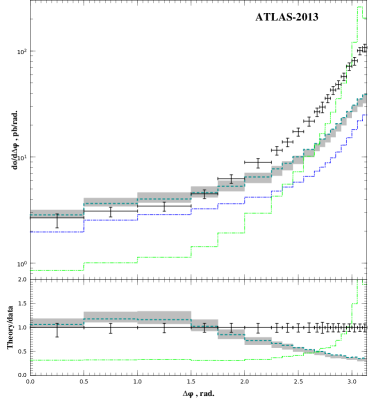
Figure 9: The $p_{T}$-spectra (left panel) and $\Delta\phi$-spectra (right panel) for the ATLAS-2013 dataset. The notation for the curves is the same as in the Fig. 8, except the thin dash-double-dotted curve, which is the Diphox (NLO CPM) prediction, taken from the Ref. ATLAS_data_2013 , see the text for details.

In the Fig. 8 the $p_{T}$-spectra of the photon pair, measured by the CDF Collaboration is presented. For this dataset, three data samples are provided, the inclusive one and two data samples with the additional kinematical constraint $p_{T}<M$ or $p_{T}>M$ imposed. One can note, that the inclusive data and data for the $p_{T}<M$ are well described for the $p_{T}>25$ GeV by the sum of the LO contribution (5) and NLO contribution (7) after the mMRK subtraction. For the $p_{T}>M$ data are well described by our prediction for all values of $p_{T}$, and the NLO contribution is, in fact, negligible. The contribution of the box subprocess (17) is only about $15\%$ of the cross section predicted at small $p_{T}$, and decreases with $p_{T}$ very fast, contributing significantly only for the $p_{T}<30$ GeV.

For the $p_{T}<25$ GeV one can observe the deficit of the predicted cross section which reaches up to a factor of $5$ at the $p_{T}=7$ GeV. The region of small-$p_{T}$ corresponds to the kinematics of CPM, where the radiation of soft gluons and virtual corrections are dominating. We expect, that computation of the NLO real-virtual interference correction in the PRA will significantly reduce this gap. One of the advantages of PRA is that at NLO this correction is finite and can be considered separately from the real NLO corrections, which are the subject of the present study.

The good description of the data for the $p_{T}>M$ region supports the self-consistency of our approach, since the NLO correction in this region is almost canceled by the mMRK subtraction terms and the contribution of the real-virtual NLO correction is expected to be small here.

For the reader’s convinience, in the figs. 8 – 12, we also have plotted the corresponding NLO CPM predictions. Data for these plots correspond to the Diphox predictions Diphox , presented in the CDF CDF_data_2012 and ATLAS ATLAS_data_2013 experimental papers. The contribution of the $gg\to\gamma\gamma$ subprocess is also included into this predictions, via GAMMA2MC program Bern_gg_gaga . Comparing the NLO CPM and NLO^⋆ PRA predictions in the figs. 8 – 12 one can conclude, that, NLO^⋆ approximation in PRA can not describe the data on the $d\sigma/dM$-distribution due to the absence of the loop correction, which contributes mostly in the back-to-back CPM-like kinematics. But for the configurations far away from the CPM kinematics, NLO^⋆ PRA describes data substantially better than NLO CPM, especially at the LHC. Moreover, in this region, the NLO^⋆ PRA prediction is dominated by the LO term, which demonstrates the better stability of PRA predictions for the kinematics far away from CPM one. Inclusion of full NLO corrections should also improve the agreement in the CPM region.

In the left panel of the Fig. 9 one can observe the same qualitative features as in the left panel of the Fig. 8, despite the fact, that we have moved from Tevatron to the LHC with it’s $3.6$ times larger energy, and switched to $pp$ collisions instead of $p\bar{p}$ ones. The NLO subprocess (7) is more important at the LHC than at the Tevatron, contributing significantly up to $p_{T}=200$ GeV.

In the Fig. 10 and right panel of the Fig. 9 the $\Delta\phi$-spectra for the Tevatron and LHC are presented. In the both figures one can observe a good agreement of our predictions with data for $\Delta\phi<1.5$ which corresponds to the high deviation from the back-to-back kinematics for the photons. In this region the NLO correction is manifestly subleading, as it was for the $p_{T}$-spectrum. The good description of the Tevatron data for the $p_{T}>M$ case is also there, as well, as the deficit of the predicted cross section for the back-to-back kinematics.

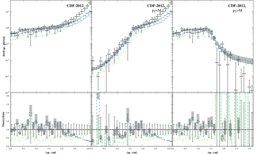
Figure 10: The $\Delta\phi$-spectra for the CDF-2012 dataset. The notation for the curves is the same as in the Fig. 8.

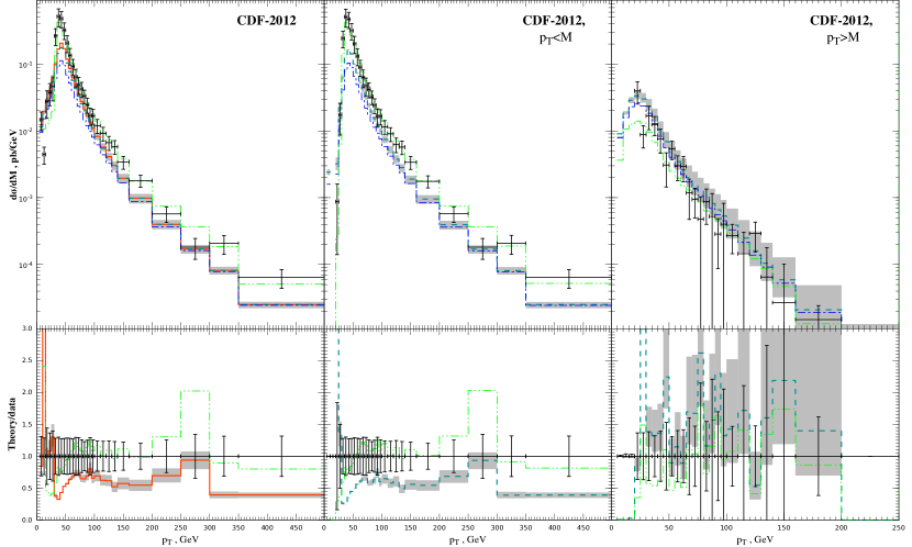
Figure 11: Diphoton invariant mass spectra for the CDF-2012 dataset. The notation for the curves is the same as in the Fig. 8

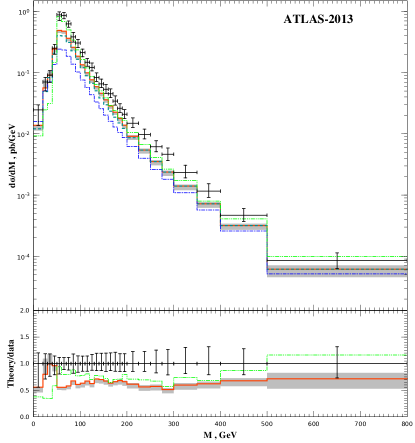
Figure 12: Diphoton invariant mass spectrum for the ATLAS-2013 dataset. The notation for the curves is the same as in the Fig. 8

As for the $M$-spectra of the Figs. 11 and 12, one certainly expects the deficit of the calculated cross section for the most values of $M$ due to the deficit of the cross section for the CPM kinematics, observed earlier, since most of the total cross section is accumulated near the CPM configurations. However, in the region of $M$ below the peak, the data are well described, demonstrating that PRA is suitable for the description of the effects of kinematical cuts. Once again, we observe the good description of the $M$-spectrum for the $p_{T}>M$ subset of the Tevatron data.

The contribution of the quark-box subprocess 17 to the $M$-spectra is found to be only about $8\%$ of the observed cross section in the peak, and $18\%$ of the predicted cross section, both for the CDF-2012 and ATLAS-2013 kinematics. This result is $20-30\%$ smaller than the usual CPM estimate 2gNNLO , which is in accordance with the findings of the Ref. KNS_photon_jet where it was shown, that the space-like virtuality of the initial-state partons suppresses the $\gamma R\to\gamma g$ contribution with respect to CPM expectation.

VI Conclusions

In the present study, the pair hadroproduction of prompt photons is considered in the framework of PRA with tree-level NLO corrections (7, 8) and NNLO quark-box subprocess (17) taken into account. The procedure of localization in rapidity of the tree-level NLO corrections to avoid the double counting the real emissions between the hard-scattering part of the cross section and unPDF is proposed in the Sec. III. As a consequence of this procedure, the real NLO corrections are put under quantitative control, and their contribution was found to be numerically small at high $p_{T}$ or in the kinematical region $p_{T}>M$. The kinematical region $p_{T}>M$ is interesting for the further theoretical and experimental study, as an ideal testing site for the PRA, where the MRK between the ISR and the hard subprocess is dominating. The contribution of the quark-box subprocess (17) was found to be about $8\%$ of the observed cross section in the peak of the $d\sigma/dM$ distribution, which is a bit smaller than the CPM estimate 2gNNLO due to the space-like virtuality of the initial-state partons, similarly to the results of the Ref. KNS_photon_jet .

References

- (1) G. Aad et al. [ATLAS Collaboration], Phys. Lett. B 716, 1 (2012) [arXiv:1207.7214 [hep-ex]]; S. Chatrchyan et al. [CMS Collaboration], Phys. Lett. B 716, 30 (2012) [arXiv:1207.7235 [hep-ex]].
- (2) ATLAS Collaboration, G. Aad et al., Phys. Rev. Lett. 113, no. 17, 171801 (2014) [arXiv:1407.6583 [hep-ex]].
- (3) T. Aaltonen et al. [CDF Collaboration], Phys. Rev. D 84, 052006 (2011) [arXiv:1106.5131 [hep-ex]]; Phys. Rev. Lett. 110, no. 10, 101801 (2013) [arXiv:1212.4204 [hep-ex]].
- (4) ATLAS Collaboration, G. Aad et al., JHEP 1301, 086 (2013) [arXiv:1211.1913 [hep-ex]].
- (5) CDF Collaboration, T. Aaltonen et al., Phys. Rev. D 80, 111106 (2009) [arXiv:0910.3623 [hep-ex]].
- (6) ATLAS Collaboration, G. Aad et al., Phys. Rev. D 89, no. 5, 052004 (2014) [arXiv:1311.1440 [hep-ex]].
- (7) CMS Collaboration, S. Chatrchyan et al., Phys. Rev. D 84, 052011 (2011) [arXiv:1108.2044 [hep-ex]].
- (8) S. Catani, M. Fontannaz, J. P. Guillet and E. Pilon, JHEP 0205, 028 (2002) [hep-ph/0204023]; P. Aurenche, M. Fontannaz, J. P. Guillet, E. Pilon and M. Werlen, Phys. Rev. D 73, 094007 (2006) [hep-ph/0602133].
- (9) V. A. Saleev, Phys. Rev. D 78, 034033 (2008) [arXiv:0807.1587 [hep-ph]].
- (10) B. A. Kniehl, V. A. Saleev, A. V. Shipilova and E. V. Yatsenko, Phys. Rev. D 84, 074017 (2011) [arXiv:1107.1462 [hep-ph]].
- (11) T. Binoth, J. P. Guillet, E. Pilon and M. Werlen, Eur. Phys. J. C 16, 311 (2000) [hep-ph/9911340].
- (12) S. Catani, L. Cieri, D. de Florian, G. Ferrera and M. Grazzini, Phys. Rev. Lett. 108, 072001 (2012) [arXiv:1110.2375 [hep-ph]].
- (13) J. C. Collins, Foundations of Perturbative QCD, Cambridge University Press, Cambridge U.K. (2011).
- (14) T. Becher, M. Neubert and D. Wilhelm, JHEP 1202, 124 (2012) [arXiv:1109.6027 [hep-ph]].
- (15) M. Anselmino, M. Boglione, J. O. Gonzalez Hernandez, S. Melis and A. Pokudin, JHEP 1404, 005 (2014)
- (16) F. Landry, R. Brock, P. M. Nadolsky and C. P. Yuan, Phys. Rev. D 67, 073016 (2003) [hep-ph/0212159]
- (17) L. V. Gribov, E. M. Levin, and M. G. Ryskin, Phys. Rept. 100, 1 (1983); J. C. Collins and R. K. Ellis, Nucl. Phys. B360, 3 (1991); S. Catani, M. Ciafaloni, and F. Hautmann, Nucl. Phys. B366, 135 (1991).
- (18) M. Ciafaloni, Nucl. Phys. B296, 49 (1988); S. Catani, F. Fiorani, and G. Marchesini, Nucl. Phys. B336, 18 (1990); Phys. Lett. B 234, 339 (1990); G. Marchesini, Nucl. Phys. B445, 49 (1995) [hep-ph/9412327].
- (19) V. A. Saleev, Phys. Rev. D 80, 114016 (2009) [arXiv:0911.5517 [hep-ph]].
- (20) A. V. Lipatov, JHEP 1302, 009 (2013) [JHEP 1302, 009 (2013)] [arXiv:1210.0823 [hep-ph]].
- (21) E. L. Berger, E. Braaten, and R. D. Field, Nucl. Phys. B 239, 52 (1984).
- (22) CDF Collaboration, D. Acosta et al., Phys. Rev. Lett. 95, 022003 (2005) [hep-ex/0412050].
- (23) V. Costantini, B. De Tollis, and G. Pistoni, Nuovo Cim. A 2, 733 (1971); V. N. Baier, V. S. Fadin, V. M. Katkov, and E. A. Kuraev, Phys. Lett. B 49, 385 (1974).
- (24) Z. Bern, L. J. Dixon and C. Schmidt, Isolating a light Higgs boson from the diphoton background at the CERN LHC, Phys. Rev. D 66, 074018 (2002) [hep-ph/0206194].
- (25) J. C. Collins, D. E. Soper and G. F. Sterman, Nucl. Phys. B 261, 104 (1985); G. T. Bodwin, Phys. Rev. D 31, 2616 (1985) [Phys. Rev. D 34, 3932 (1986)]; 34, 3932(E) (1986)
- (26) L. N. Lipatov, Yad. Fiz. 23, 642 (1976) [Sov. J. Nucl. Phys. 23, 338 (1976)]; E. A. Kuraev, L. N. Lipatov, and V. S. Fadin, Zh. Eksp. Teor. Fiz. 71, 840 (1976) [Sov. Phys. JETP 44, 443 (1976)]; Zh. Eksp. Teor. Fiz. 72, 377 (1977) [Sov. Phys. JETP 45, 199 (1977)]; I. I. Balitsky and L. N. Lipatov, Yad. Fiz. 28, 1597 (1978) [Sov. J. Nucl. Phys. 28, 822 (1978)]; Zh. Eksp. Teor. Fiz. 90, 1536 (1986) [Sov. Phys. JETP 63, 904 (1986)].
- (27) L. N. Lipatov, Phys. Rept. 286, 131 (1997) [hep-ph/9610276].
- (28) B. L. Ioffe, V. S. Fadin, L. N. Lipatov, Quantum Chromodynamics: Perturbative and Nonperturbative Aspects, Cambridge University Press, Cambridge U.K. (2010).
- (29) V. S. Fadin and V. E. Sherman, JETP Lett. 23, 599 (1976); JETP 45, 861 (1977).
- (30) A. V. Bogdan and V. S. Fadin, Nucl. Phys. B 740, 36 (2006) [hep-ph/0601117].
- (31) L. N. Lipatov, Nucl. Phys. B452, 369 (1995) [hep-ph/9502308].
- (32) L. N. Lipatov and M. I. Vyazovsky, Nucl. Phys. B597, 399 (2001) [hep-ph/0009340].
- (33) E. N. Antonov, L. N. Lipatov, E. A. Kuraev, and I. O. Cherednikov, Nucl. Phys. B721, 111 (2005) [hep-ph/0411185].
- (34) A. van Hameren, K. Kutak and T. Salwa, Phys. Lett. B 727, 226 (2013) [arXiv:1308.2861 [hep-ph]].
- (35) A. van Hameren, JHEP 1407, 138 (2014) [arXiv:1404.7818 [hep-ph]].
- (36) V. N. Gribov and L. N. Lipatov, Yad. Fiz. 15, 781 (1972) [Sov. J. Nucl. Phys. 15, 438 (1972)]; Yu. L. Dokshitzer, Zh. Eksp. Teor. Fiz. 73, 1216 (1977) [Sov. Phys. JETP 46, 641 (1977)]; G. Altarelli and G. Parisi, Nucl. Phys. 126, 298 (1977).
- (37) J. Blümlein, DESY Report No. 95-121 (1995) [hep-ph/9506403].
- (38) M. A. Kimber, A. D. Martin, and M. G. Ryskin, Eur. Phys. J. C 12, 655 (2000) [hep-ph/9911379]; Phys. Rev. D 63, 114027 (2001) [hep-ph/0101348]; G. Watt, A. D. Martin, and M. G. Ryskin, Eur. Phys. J. C 31, 73 (2003) [hep-ph/0306169]; Phys. Rev. D 70, 014012 (2004); 70, 079902(E) (2004) [hep-ph/0309096].
- (39) A. V. Karpishkov, M. A. Nefedov, V. A. Saleev and A. V. Shipilova, Phys. Rev. D 91, no. 5, 054009 (2015) [arXiv:1410.7139 [hep-ph]].
- (40) A. V. Karpishkov, M. A. Nefedov, V. A. Saleev and A. V. Shipilova, Int. J. Mod. Phys. A 30, no. 04n05, 1550023 (2015) [arXiv:1411.7672 [hep-ph]].
- (41) F. Hautmann, H. Jung, M. Krämer, P. J. Mulders, E. R. Nocera, T. C. Rogers and A. Signori, Eur. Phys. J. C 74, no. 12, 3220 (2014) [arXiv:1408.3015 [hep-ph]].
- (42) A. D. Martin, M. G. Ryskin and G. Watt, Eur. Phys. J. C 66, 163 (2010) [arXiv:0909.5529 [hep-ph]].
- (43) J. Bartels, A. Sabio Vera and F. Schwennsen, JHEP 0611, 051 (2006) [hep-ph/0608154].
- (44) M. Hentschinski and A. S. Vera, Phys. Rev. D 85, 056006 (2012) [arXiv:1110.6741 [hep-ph]].
- (45) T. Hahn, Comput. Phys. Commun. 140, 418 (2001) [hep-ph/0012260].
- (46) R. Mertig, M. Bohm and A. Denner, Comput. Phys. Commun. 64, 345 (1991).
- (47) L. Cieri, D. de Florian, arXiv:1405.1067 [hep-ph].
- (48) S. Frixione, Phys. Lett. B 429, 369 (1998) [hep-ph/9801442].
- (49) J. R. Andersen, V. Del Duca and C. D. White, JHEP 0902, 015 (2009) [arXiv:0808.3696 [hep-ph]]; J. R. Andersen and J. M. Smillie, JHEP 1001, 039 (2010) [arXiv:0908.2786 [hep-ph]].
- (50) A. D. Martin, W. J. Stirling, R. S. Thorne and G. Watt, Parton distributions for the LHC, Eur. Phys. J. C 63, 189 (2009) [arXiv:0901.0002 [hep-ph]].
- (51) T. Hahn, Comput. Phys. Commun. 168, 78 (2005) [hep-ph/0404043].
- (52) B. A. Kniehl, M. A. Nefedov and V. A. Saleev, Phys. Rev. D 89, no. 11, 114016 (2014) [arXiv:1404.3513 [hep-ph]].