Flat-band ferromagnetism in a topological Hubbard model

Abstract

We study the flat-band ferromagnetic phase of a topological Hubbard model within a bosonization formalism and, in particular, determine the spin-wave excitation spectrum. We consider a square lattice Hubbard model at $1/4$-filling whose free-electron term is the $\pi$-flux model with topologically nontrivial and nearly flat energy bands. The electron spin is introduced such that the model either explicitly breaks time-reversal symmetry (correlated flat-band Chern insulator) or is invariant under time-reversal symmetry (correlated flat-band Z₂ topological insulator). We generalize for flat-band Chern and topological insulators the bosonization formalism [Phys. Rev. B 71, 045339 (2005)] previously developed for the two-dimensional electron gas in a uniform and perpendicular magnetic field at filling factor $\nu=1$. We show that, within the bosonization scheme, the topological Hubbard model is mapped into an effective interacting boson model. We consider the boson model at the harmonic approximation and show that, for the correlated Chern insulator, the spin-wave excitation spectrum is gapless while, for the correlated topological insulator, gapped. We briefly comment on the possible effects of the boson-boson (spin-wave–spin-wave) coupling.

I Introduction

Electronic bands with non-zero Chern numbers are at the origin of a large variety of topological phenomena in condensed-matter systems.hasan10 ; kane13 In a pioneering work in 1988, Haldane showed that a two-dimensional graphene-like lattice model with broken time-reversal symmetry can exhibit an integer quantum Hall effect (IQHE) without an external magnetic field.haldane88 Later, in 2005, Kane and Mele generalized this model to restore time-reversal symmetry with the help of the natural spin degree of freedom in graphene with spin-orbit coupling.kane05 ; kane05-1 The lowest-energy spin bands in this model carry non-zero but opposite Chern numbers that result in the quantum spin Hall effect (QSHE), which manifests itself in a quantized conductance associated with the transverse spin current. Whereas the intrinsic spin-orbit coupling is too small in graphene to reveal the effect, the QSHE was later predictedbhz06 to occur and measuredkonig in HgTe/CdTe quantum wells.

The presence of an IQHE in a band with a non-zero Chern number indicates a certain similarity between the band and the Landau level of the two-dimensional electron gas (2DEG) in a strong magnetic field. However, in contrast to the latter the energy bands obtained in tight-binding models have usually a non-negligible dispersion. In order to investigate in further details the relation between Landau levels and energy bands with non-zero Chern numbers, special effort has recently been invested into the engineering of flat bands in specially designed tight-binding models.tang11 ; sun11 ; neupert11 If these bands are partially filled and if electron-electron interactions are taken into account, one would then expect correlation effects similar to the fractional quantum Hall effect (FQHE). The effect, also called fractional Chern insulator, was later corroborated within numerical studiessheng11 ; regnault11 (for recent reviews, see sondhi13, ; liu13, ; neupert13, ).

The analogy between flat bands with non-zero Chern number and Landau levels can be pushed further when the internal spin degree of freedom is taken into account. Indeed, when there are as many electrons as flux quanta threading the 2DEG, the spins are spontaneously aligned and form a ferromagnetic state (quantum Hall ferromagnet) in order to minimize the electron-electron repulsion.ezawa This situation corresponds to half-filling in a lattice model if only the two lowest (spin) bands are taken into account. However, in contrast to Landau levels, where time-reversal symmetry is broken by the external magnetic field and the Landau levels occur merely in two spin copies, the situation is more involved in lattice models. One needs to distinguish two generic situations. In the first one, time-reversal symmetry is preserved such that spin and orbital degrees of freedom are coupled. In this case, possible spin excitations are described in the framework of rather unusual commutation relations for the spin-density operatorsgoerbig12 and the resulting ferromagnetic state is expected to respect the underlying Z₂ symmetry of topological insulators.kane05 This type of ferromagnetism has recently been investigated within numerical exact-diagonalization studies by Neupert et al., who find a gapped Ising ferromagnetic ground state.neupert12 The second situation arises when time-reversal symmetry is broken on the level of the lattice model, and where the Chern bands occur in two spin copies without any spin-orbit structure.

In the present paper, we investigate ferromagnetism in both situations, within a specially adapted tight-binding model on a square lattice with on-site Hubbard repulsion that is a generalization of the model originally presented in Ref. neupert11, . The tight-binding model, in the absence of interactions, bears a staggered $\pi$-flux phase for each spin component, and time-reversal symmetry determines whether the two spin species experience either the same or an opposite flux per plaquette. If time-reversal symmetry is broken, one is confronted with a correlated flat-band Chern insulator, whereas one finds a correlated flat-band Z₂ topological insulator in the case of preserved time-reversal symmetry. For both situations, we investigate the ferromagnetic state at quarter-filling of the lattice that corresponds to half-filling of the two lowest energy bands. In order to investigate its stability and collective spin-wave excitations, we construct a nonpertubartive bosonization scheme similar to the one proposed in Ref. doretto05, to describe the 2DEG at filling factor $\nu=1$. Such a formalism was also applied to study quantum Hall ferromagnetic phases realized in graphene at filling factors $\nu=0$ and $\nu=\pm 1$doretto07 and to describe the Bose-Einstein condensate of magnetic excitons realized in a bilayer quantum Hall system at total filling factor $\nu_{T}=1$.doretto06 ; doretto12

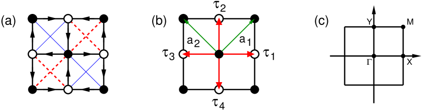
Figure 1: (Color online) (a) Schematic representation of the hopping term (1). The nearest-neighbor hopping energies (solid black lines) are equal to $t_{1}\exp\left(i\pi/4\right)$ (spin up electrons) in the direction of the arrows and the next-nearest-neighbor hopping energies are equal to $+t_{2}$ (dashed red lines) and $-t_{2}$ (thin blue lines). Black and open circles indicate sites of the $A$ and $B$ sublattices, respectively. (b) The nearest-neighbor vectors $\mbox{\boldmath$\tau$}_{i}$ [read arrows, Eq. (LABEL:tauvectors)] and the primitive vectors ${\mathbf{a}}_{1}=a\hat{x}$ and ${\mathbf{a}}_{2}=a\hat{y}$ [green arrows, Eq. (5)]. The next-nearest neighbor distance $a$ is set to one. (c) Brillouin zone. Here ${\bf X}=(\pi,0)$, ${\bf Y}=(0,\pi)$, and ${\bf M}=(\pi,\pi)$.

I.1 Overview of the results

We show that the bosonization scheme,doretto05 originally developed for the 2DEG at filling factor $\nu=1$, can be generalized for lattice models that describe flat-band Chern and Z₂ topological insulators.

For both correlated Chern and Z₂ topological insulators described above, we map the interacting fermion model to an effective interacting boson model. We consider the effective boson model in the harmonic approximation and show that the ground state is indeed given by a spin polarized (ferromagnetic) state. Our main results are in fact the analytical calculation of the spin-wave excitation spectra of both ferromagnets (Figs. 4 and 5). The spin-wave dispersion relation corresponds to the energy of the bosons at the harmonic approximation. Due to the bipartite nature of the underlying square lattice, we identify two types of collective spin-wave excitations. We find that the correlated flat-band Chern insulator has one gapless and one gapped spin-wave excitation branches (Fig. 4) while the correlated flat-band topological insulator, two gapped ones (Fig. 5). For the latter, the excitation gap we obtain at zero-wave vector coincides with the result numerically calculated by Neupert et al.neupert12

I.2 Outline

Our paper is organized as follows. Section II introduces the basic tight-binding model (the spinfull square lattice $\pi$-flux model), which is discussed in view of the role played by time-reversal symmetry. We discuss the flat-band ferromagnetic phase of a correlated Chern insulator with broken time-reversal symmetry in Sec. III, whereas the more involved case of a model with underlying time-reversal symmetry (correlated topological insulator) is presented in Sec. IV. For both cases, the particularities of the associated lattice models are first discussed in Secs. III.1 and IV.1 before we present the details of the bosonization schemes in Sec. III.2 and Sec. IV.2, respectively. The bosonization formalism is then applied in Secs. III.3 and IV.3 to study the flat-band ferromagnetic phases obtained in the presence of a strong on-site Hubbard repulsion term in the respective models. We comment on possible extensions of the bosonization scheme and the effects of the boson-boson (spin-wave–spin-wave) coupling in Sec. V and, in Sec. VI, we provide a brief summary of our findings. Technical details of the two bosonization schemes, as well as a more detailed analysis of time-reversal symmetry, are delegated to the (three) Appendices.

II Tight-binding models with flat topological bands

Before a detailed analysis of the different ferromagnetic states in flat-band Chern insulators with broken time-reversal symmetry and Z₂ topological insulators, we present here a common tight-binding model that provides the different flat bands.

Let us consider $N_{e}=N$ free spin-$1/2$ electrons hopping on a bipartite square lattice where both sublattices $A$ and $B$ have each $N_{A}=N_{B}=N$ sites. The Hamiltonian of the system is given by the tight-binding model

$$\mathcal{H}_{0} = \sum_{i\in A,\,n,\,\sigma}\left(t_{i,i+n,\sigma}\,c^{\dagger}_{i\,A\,\sigma}c_{i+n\,B\,\sigma}+{\rm H.c.}\right)$$ (1)

$$+ \sum_{i,\,\delta,\,a,\,\sigma}\left(\lambda_{i,i+\delta}\,c^{\dagger}_{i\,a\,\sigma}c_{i+\delta\,a\,\sigma}+{\rm H.c.}\right).$$

Here $c^{\dagger}_{i\,a\,\sigma}$ ($c_{i\,a\,\sigma}$) creates (destroys) a spin $\sigma=\uparrow,\downarrow$ electron on site $i$ of the sublattice $a=A,B$. The spin-dependent nearest-neighbor $t_{i,j,\sigma}$ and next-nearest-neighbor $\lambda_{i,j}$ hopping energies are respectively given by [Fig. 1(a)]

$$t_{i,i+n,\sigma}=t_{1}\exp\left[i(-1)^{n}\gamma(\sigma)\pi/4\right],\;\;\;\;i\in A,$$ (2)

$$\lambda_{i,i+\delta}=\left\{\begin{tabular}[]{ll}$-(-1)^{\delta}t_{2}$,&$\;\;i\in A$,\\ $+(-1)^{\delta}t_{2}$,&$\;\;i\in B$,\end{tabular}\right.$$ (3)

where $t_{1}$ and $t_{2}$ are positive real quantities. The indices $n=1,2,3,4$ correspond to the nearest-neighbor vectors [Fig. 1(b)]

$$\mbox{\boldmath$\tau$}_{1} = -\mbox{\boldmath$\tau$}_{3}=\frac{1}{2}\left({\mathbf{a}}_{1}-{\mathbf{a}}_{2}\right)=\frac{a}{2}(\hat{x}-\hat{y}),$$

$$\mbox{\boldmath$\tau$}_{2} = -\mbox{\boldmath$\tau$}_{4}=\frac{1}{2}\left({\mathbf{a}}_{1}+{\mathbf{a}}_{2}\right)=\frac{a}{2}(\hat{x}+\hat{y}),$$

and $\delta$ is either $1$ or $2$ corresponding to the next-nearest-neighbor vectors

$$\mbox{\boldmath$\delta$}_{1}={\mathbf{a}}_{1}=a\hat{x},\;\;\;\;\;\;\;\mbox{\boldmath$\delta$}_{2}={\mathbf{a}}_{2}=a\hat{y}.$$ (5)

In the remainder of this paper, we set the next-nearest-neighbor distance $a=1$. The spin-dependent phases $\gamma(\sigma)$ reflect that time-reversal symmetry is preserved for $\gamma(\uparrow)=-\gamma(\downarrow)=1$, whereas it is broken if $\gamma(\uparrow)=\gamma(\downarrow)=1$ (see Appendix A for details). The tight-binding model (1) is a generalization for the case of electrons with spin of the $\pi$-flux model discussed in Ref. neupert11, . Since the nearest-neighbor hopping energy (2) is complex, each electron acquires a phase $\pi$ as it hops around a plaquette in the direction of the arrows indicated in Fig. 1(a). Therefore, $\mathcal{H}_{0}$ describes noninteracting electrons hopping in a square lattice in the presence of a fictitious staggered $\pm\pi$ flux pattern.lee06 For the time-reversal-symmetric model [$\gamma(\uparrow)=-\gamma(\downarrow)=1$] the flux experienced by electrons of opposite spin is opposite, whereas it is the same for $\gamma(\uparrow)=\gamma(\downarrow)=1$, i.e., in the case of broken time-reversal symmetry.

After Fourier transformation, i.e., introducing

$$c^{\dagger}_{i\,a\,\sigma}=\frac{1}{N^{1/2}_{a}}\sum_{{\bf k}\in{\rm BZ}}\exp(-i{\bf k}\cdot{\bf R}_{i})c^{\dagger}_{{\bf k}\,a\,\sigma}$$ (6)

with the momentum sum running over the BZ associated with the underlying Bravais lattice [see Fig. 1(c)], it is possible to show that the hopping term (1) assumes the form

$$\mathcal{H}_{0}=\sum_{{\bf k}\in BZ}\Psi^{\dagger}_{\bf k}\mathcal{H}_{\bf k}\Psi_{\bf k},$$ (7)

where

$$\mathcal{H}_{k}=\left(\begin{array}[]{cc}h^{\uparrow}_{\bf k}&0\\ 0&h^{\downarrow}_{\bf k}\end{array}\right)$$ (8)

is a $4\times 4$ matrix and

$$\Psi^{\dagger}_{\bf k}=\left(c^{\dagger}_{{\bf k}\,A\,\uparrow}\;\;c^{\dagger}_{{\bf k}\,B\,\uparrow}\;\;c^{\dagger}_{{\bf k}\,A\,\downarrow}\;\;c^{\dagger}_{{\bf k}\,B\,\downarrow}\right)$$ (9)

is a four-component spinor. Furthermore,

$$h^{\uparrow}_{\bf k}=B_{0,{\bf k}}\tau_{0}+{\bf B}_{\bf k}\cdot\hat{\tau}$$ (10)

is a $2\times 2$ matrix where $\tau_{0}=I_{2\times 2}$ is the identity matrix and $\hat{\tau}=(\tau_{1},\tau_{2},\tau_{3})$ is a vector whose components are the Pauli matrices. Finally, $B_{0,{\bf k}}$ and the components of the vector ${\bf B}_{\bf k}=(B_{1,{\bf k}},B_{2,{\bf k}},B_{3,{\bf k}})$ are given by the functions

$$B_{0,{\bf k}} = 0,$$

$$B_{1,{\bf k}} = 2\sqrt{2}t_{1}\cos\frac{k_{x}}{2}\cos\frac{k_{y}}{2},$$

$$B_{2,{\bf k}} = 2\sqrt{2}t_{1}\gamma(\sigma)\sin\frac{k_{x}}{2}\sin\frac{k_{y}}{2},$$

$$B_{3,{\bf k}} = 2t_{2}\left(\cos k_{x}-\cos k_{y}\right).$$ (11)

Again, the factor $\gamma(\sigma)$ indicates whether time-reversal symmetry is broken or not. Whereas the time-reversal-symmetric model [$\gamma(\uparrow)=-\gamma(\downarrow)=1$] has the usual property $h_{{\bf k}}^{\uparrow}=(h_{-{\bf k}}^{\downarrow})^{*}$, we find that the two components of the Hamiltonian (8) are identical for all wave vectors, $h^{\downarrow}_{\bf k}=h^{\uparrow}_{\bf k}$, in the case of $\gamma(\uparrow)=\gamma(\downarrow)=1$.

II.1 Symmetries of the $\pi$-flux model: spin rotation

The above discussion and the role of time-reversal symmetry allow us to investigate certain properties of the supposed flat-band ferromagnetic states from a pure symmetry point of view. In this section, we discuss the behavior of the noninteracting fermion model (1) under spin rotation. Some further considerations about the behavior of (1) under time-reversal are present in Appendix A.

The Hamiltonian (7) can indeed be written as

$$\mathcal{H}_{0} = \sum_{{\bf k},\sigma}\sum_{a,b}E^{ab}_{\sigma}({\bf k})c^{\dagger}_{{\bf k}\,a\,\sigma}c_{{\bf k}\,b\,\sigma}.$$ (12)

Comparing Eq. (12) with Eqs. (8) and (10), we see that, for the Chern insulator with broken time-reversal symmetry ($h^{\uparrow}_{\bf k}=h^{\downarrow}_{\bf k}$),

$$E^{aa}_{\uparrow}({\bf k})=E^{aa}_{\downarrow}({\bf k})\;\;\;\;{\rm and}\;\;\;\;E^{ab}_{\uparrow}({\bf k})=E^{ab}_{\downarrow}({\bf k})$$ (13)

with $a\not=b$, while for the topological insulator with time-reversal symmetry ($h^{\downarrow}_{\bf k}=h^{\uparrow\,*}_{-{\bf k}}$), we have

$$E^{aa}_{\uparrow}({\bf k})=E^{aa}_{\downarrow}({\bf k})\;\;\;\;{\rm and}\;\;\;\;E^{ab}_{\uparrow}({\bf k})\not=E^{ab}_{\downarrow}({\bf k})$$ (14)

with $a\not=b$.

The total spin operator reads

$${\bf S}=\sum_{i,a}{\bf S}_{i\,a}=\frac{1}{2}\sum_{a,{\bf p}}c^{\dagger}_{{\bf p}\,a\,\sigma}\hat{\sigma}_{\sigma,\sigma^{\prime}}c_{{\bf p}\,a\,\sigma^{\prime}}$$ (15)

where ${\bf S}_{i\,a}$ is the spin operator at site $i$ of the sublattice $a$ and $\hat{\sigma}=(\sigma_{1},\sigma_{2},\sigma_{3})$ is a vector of Pauli matrices associated with the physical spin [see Eq. (25) below]. It is possible to show that the following commutation relations hold:

$$[\mathcal{H}_{0},S^{z}] = 0$$

$$\,[\mathcal{H}_{0},S^{+}] = \sum_{\bf k}\sum_{a}\left[E^{aa}_{\uparrow}({\bf k})-E^{aa}_{\downarrow}({\bf k})\right]c^{\dagger}_{{\bf k},\,a\,\uparrow}c_{{\bf k},\,a\,\downarrow}$$

$$+\left[E^{AB}_{\uparrow}({\bf k})-E^{AB}_{\downarrow}({\bf k})\right]c^{\dagger}_{{\bf k},\,A\,\uparrow}c_{{\bf k},\,B\,\downarrow}$$

$$+\left[E^{BA}_{\uparrow}({\bf k})-E^{BA}_{\downarrow}({\bf k})\right]c^{\dagger}_{{\bf k},\,B\,\uparrow}c_{{\bf k},\,A\,\downarrow},$$

$$\,[\mathcal{H}_{0},S^{-}] = [S^{+},\mathcal{H}_{0}]^{*}.$$ (16)

Since the Chern insulator is characterized by the Hamiltonian (8) with two identical components for the two spin orientations [see Eq. (13)], one immediately realizes that all components of the total spin operator (15) commute with the Hamiltonian (8), i.e., the Hamiltonian has SU(2) spin rotation symmetry. In the case of a ferromagnetic ground state that breaks spin rotation symmetry, all equivalent states can thus be obtained by global rotations generated by the total spin operator (15), and one would therefore expect the presence of a Goldstone mode in the spin-wave excitation spectrum. We show explicitly in the following section the existence of such a mode.

Concerning a topological insulator described by the Hamiltonian (8) with coefficients obeying Eq. (14), one can easily see that the SU(2) spin rotation symmetry is now explicitly broken to U(1), i.e., the Hamiltonian is invariant under spin rotations around the $z$-axis. Therefore, the presence of a Goldstone mode depends on the ground-state spin polarization: whereas one would expect a superfluid-type mode for an easy-plane ferromagnetic state, where the polarization is oriented in the $xy$-plane, an easy-axis ferromagnet with a polarization along the $z$-direction would not display a Goldstone mode since the ground state preserves the U(1) spin rotation symmetry of the Hamiltonian. In the following, we show that the latter is the case for a topological insulator and that all collective excitations are indeed gapped.

III Ferromagnetism in a flat-band Chern insulator

In this section, we discuss the flat-band ferromagnetic phase of a topological Hubbard model that explicitly breaks time-reversal symmetry. We start by discussing the free electron term of the model.

III.1 Square lattice $\pi$-flux model with broken time-reversal symmetry

The noninteracting Hamiltonian (7) with $\gamma(\uparrow)=\gamma(\downarrow)=1$ can be diagonalized with the aid of the Bogoliubov transformation

$$c^{\dagger}_{{\bf k}\,A\,\sigma} = u_{\bf k}d^{\dagger}_{{\bf k}\,\sigma}+v^{*}_{\bf k}c^{\dagger}_{{\bf k}\,\sigma},$$

$$c^{\dagger}_{{\bf k}\,B\,\sigma} = v_{\bf k}d^{\dagger}_{{\bf k}\,\sigma}-u^{*}_{\bf k}c_{{\bf k}\,\sigma},$$ (17)

where the Bogoliubov coefficients $u_{\bf k}$ and $v_{\bf k}$ are given by Eq. (87). After diagonalization, the Hamiltonian (7) assumes the form [see Eqs. (87)-(89) for details]

$$\mathcal{H}_{0}=\sum_{{\bf k}\in BZ}\Phi^{\dagger}_{\bf k}\mathcal{H^{\prime}}_{\bf k}\Phi_{\bf k},$$ (18)

where the $4\times 4$ matrix $\mathcal{H^{\prime}}_{\bf k}$ reads

$$\mathcal{H^{\prime}}_{\bf k}=\left(\begin{array}[]{cc}h^{\prime}_{\bf k}&0\\ 0&h^{\prime}_{\bf k}\end{array}\right),$$ (19)

with

$$h^{\prime}_{\bf k}=\left(\begin{array}[]{cc}\omega_{d,{\bf k}}&0\\ 0&\omega_{c,{\bf k}}\end{array}\right)$$ (20)

being a $2\times 2$ diagonal matrix whose elements are the upper band $d$ ($+$ sign) and the lower one $c$ ($-$ sign),

$$\omega_{d/c,{\bf k}}=B_{0,{\bf k}}\pm|{\bf B}_{\bf k}|,$$ (21)

and the new four component spinor $\Phi^{\dagger}_{\bf k}$ is given by

$$\Phi^{\dagger}_{\bf k}=\left(d^{\dagger}_{{\bf k}\,\uparrow}\;\;c^{\dagger}_{{\bf k}\,\uparrow}\;\;d^{\dagger}_{{\bf k}\,\downarrow}\;\;c^{\dagger}_{{\bf k}\,\downarrow}\right).$$ (22)

The band structure of $\mathcal{H}_{0}$ is made out of four bands:

$$d\uparrow,\,\,d\downarrow,\,\,c\uparrow,\,\,c\downarrow,$$

with the $c$ and $d$ bands doubly degenerate in the spin degree of freedom as expected from the discussion of the previous section. Figure 2 shows the energy of the $c$ and $d$ bands [Eq. (21)] for different values of the ratio $t_{2}/t_{1}$. Note that the spectrum is gapless for $t_{2}=0$ and, as $t_{2}$ increases, it acquires a finite energy gap $\Delta={\rm min}(\omega_{d,{\bf k}})-{\rm max}(\omega_{c,{\bf k}})$. Indeed, as shown in Fig. 3, $\Delta$ linearly increases with $t_{2}$ for $t_{2}<0.5\,t_{1}$ and then it saturates at $\Delta=4\,t_{1}$ for larger values of $t_{2}$. The widths $W_{c/d}={\rm max}(\omega_{c/d,{\bf k}})-{\rm min}(\omega_{c/d,{\bf k}})$ of the $c$ and $d$ bands also change with $t_{2}$. In particular, as illustrated in Fig. 3, the flatness ratio $f_{c}=\Delta/W_{c}$ of the $c$-bandsondhi13 is maximum ($f_{c}=4.83$) for $0.5\leq t_{2}/t_{1}\leq 1/\sqrt{2}$. Such a range includes the configuration $t_{2}=t_{1}/\sqrt{2}$ discussed by Neupert et al.neupert11

An interesting aspect of the tight-binding model $\mathcal{H}_{0}$ is that its energy bands are topologically nontrivial. Indeed, it is possible to show that the Chern numbers of the $c$ and $d$ bands can be written in terms of the coefficients $B_{i,{\bf k}}$ [Eq. (11)] and that they are finite, i.e.,hasan10 ; kane13 ; neupert11 ; assaad13

$$C^{d/c}_{\sigma}=\mp\frac{1}{4\pi}\int_{BZ}d^{2}k\;\;\hat{B}_{\bf k}\cdot(\partial_{k_{x}}\hat{B}_{\bf k}\times\partial_{k_{y}}\hat{B}_{\bf k})=\mp 1,$$ (23)

with $\hat{{\bf B}}_{\bf k}\equiv{\bf B}_{\bf k}/|{\bf B}_{\bf k}|$, regardless the value of $t_{2}>0$. Therefore, the square lattice $\pi$-flux model (1) with broken time-reversal symmetry is an example of a Chern insulator. As discussed in the Introduction, the system should exhibit an IQHE when a certain number of energy bands are completely filled.

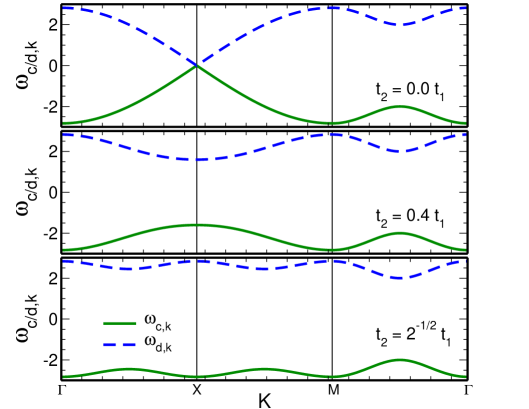
Figure 2: (Color online) Band structure of the noninteracting hopping term $\mathcal{H}_{0}$ [Eq. (21) in units of $t_{1}$] along paths in the Brillouin zone [Fig. 1(c)] for different values of the next-nearest-neighbor hopping energy amplitude $t_{2}$. Solid green and dashed blue lines correspond respectively to the $c$ and $d$ bands.

In the following, we focus on the nearly flat-band limit of $\mathcal{H}_{0}$, in particular, we consider $t_{2}=t_{1}/\sqrt{2}$. Note that since each of the $c\,\sigma$ and $d\,\sigma$ bands have $N_{A}=N_{B}=N$ available states and $N_{e}=N$, the $d$ band is empty while the $c$ one is half-filled, i.e., we have $1/4$-filling including all four bands. In the next section, we introduce a bosonization scheme to describe such a flat-band Chern insulator.

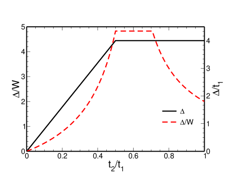
Figure 3: (Color online) Flatness ratio $\Delta/W$ of the $c$-band and band gap $\Delta$ as a function of the next-nearest-neighbor hopping energy amplitude $t_{2}$ for the noninteracting hopping term $\mathcal{H}_{0}$.

III.2 Bosonization scheme for a flat-band Chern insulator

In order to study the flat-band ferromagnetic phase of a correlated Chern insulator, we introduce a bosonization scheme similar to that proposed in Ref. doretto05, for the 2DEG at $\nu=1$. Following the lines of the bosonization method for one-dimensional fermion systems,giamarchi the idea of the formalismdoretto05 is to define boson operators in terms of the lowest energy neutral excitations of the original fermionic system and then map the interacting electronic model to an effective bosonic one. In the following, we outline the bosonization scheme for flat-band Chern insulators. The (two) approximations involved and the differences between the scheme on a lattice and the one developed for the 2DEG at $\nu=1$ are discussed. Further details can be found in Appendix B.

Let us consider the tight-binding model (1) at $1/4$-filling. As mentioned in the previous section, in this case the highest energy $d$ bands are completely empty while the lowest energy $c$ ones are half-filled, see Fig. 2. In particular, let us assume that the $c\uparrow$ band is completely filled while the $c\downarrow$ one is completely empty, i.e., we consider that the ground state of the free electron model (1) is completely spin polarized,

$$|{\rm FM}\rangle=\prod_{{\bf k}\in{\rm BZ}}c^{\dagger}_{{\bf k}\,\uparrow}|0\rangle.$$ (24)

The state $|{\rm FM}\rangle$ is the reference state of the bosonization method and belongs to the ground-state manifold of ferromagnetic states that need to be considered when electronic interactions are taken into account. Since the lowest energy $c$ bands are separated from the highest energy $d$ ones by an energy gap and the former bands are partially filled, the lowest-energy neutral excitations are given by particle-hole pairs (spin flips) within the $c$ bands. Therefore, in the following, we neglect the $d$ bands, i.e., we restrict the Hilbert space to the subspace spanned by the lowest energy $c$ bands.

The spin operator at site $i$ of the sublattice $a$ is defined as

$${\bf S}_{i\,a}=\frac{1}{2}c^{\dagger}_{i\,a\,\sigma}\hat{\sigma}_{\sigma\,\sigma^{\prime}}c_{i\,a\,\sigma^{\prime}}$$ (25)

in terms of the Pauli matrices defined above. The Fourier transform of the components of ${\bf S}_{i\,a}$ read

$$S^{\lambda}_{i\,a}=\frac{1}{N_{a}}\sum_{\bf q}\exp(i{\bf q}\cdot{\bf R}_{i})S^{\lambda}_{{\bf q},a}$$ (26)

with $\lambda=x,y,z$. In particular, using Eq. (6), it is possible to show that

$$S^{+}_{{\bf q},a} = \sum_{\bf p}c^{\dagger}_{{\bf p}-{\bf q}\,a\,\uparrow}c_{{\bf p}\,a\,\downarrow},$$

$$S^{-}_{{\bf q},a} = \sum_{\bf p}c^{\dagger}_{{\bf p}-{\bf q}\,a\,\downarrow}c_{{\bf p}\,a\,\uparrow},$$ (27)

where $S^{\pm}_{{\bf q},a}=S^{x}_{{\bf q},a}\pm iS^{y}_{{\bf q},a}$. With the help of the Bogoliubov transformation (17), one can express the spin operators $S^{\pm}_{{\bf q},a}$ in terms of the $c$ and $d$ fermion operators. For instance,

$$S^{+}_{{\bf q},A} = \sum_{\bf p}\left(u_{{\bf p}-{\bf q}}u^{*}_{\bf p}d^{\dagger}_{{\bf p}-{\bf q}\,\uparrow}d_{{\bf p}\,\downarrow}+v^{*}_{{\bf p}-{\bf q}}v_{\bf p}c^{\dagger}_{{\bf p}-{\bf q}\,\uparrow}c_{{\bf p}\,\downarrow}\right.$$ (28)

$$+ \left.u_{{\bf p}-{\bf q}}v_{\bf p}d^{\dagger}_{{\bf p}-{\bf q}\,\uparrow}c_{{\bf p}\,\downarrow}+v^{*}_{{\bf p}-{\bf q}}u^{*}_{\bf p}c^{\dagger}_{{\bf p}-{\bf q}\,\uparrow}d_{{\bf p}\,\downarrow}\right),\;$$

where $u_{\bf p}$ and $v_{\bf p}$ are the Bogoliubov coefficients (87). Note that by projecting $S^{+}_{{\bf q},A}$ into the $c$ bands, only the second term on the R.H.S. of Eq. (28) survives. Indeed, it is easy to see that the expressions of the projected spin operators $\bar{S}^{\pm}_{{\bf q},a}$ read

$$\bar{S}^{+}_{{\bf q},a} = \sum_{\bf p}G_{a}({\bf p},{\bf q})c^{\dagger}_{{\bf p}-{\bf q}\,\uparrow}c_{{\bf p}\,\downarrow},$$

$$\bar{S}^{-}_{{\bf q},a} = \sum_{\bf p}G_{a}({\bf p},{\bf q})c^{\dagger}_{{\bf p}-{\bf q}\,\downarrow}c_{{\bf p}\,\uparrow},$$ (29)

where

$$G_{A}({\bf p},{\bf q})=v^{*}_{{\bf p}-{\bf q}}v_{\bf p}\;\;\;\;{\rm and}\;\;\;\;G_{B}({\bf p},{\bf q})=u^{*}_{{\bf p}-{\bf q}}u_{\bf p}.$$ (30)

As discussed below, it is interesting to consider the following linear combination of the spin operators $\bar{S}^{\lambda}_{{\bf q},a}$:

$$\bar{S}^{\lambda}_{{\bf q},\alpha}=\bar{S}^{\lambda}_{{\bf q},A}+(-1)^{\alpha}\bar{S}^{\lambda}_{{\bf q},B}$$ (31)

with $\lambda=x,y,z$ and $\alpha=0,1$. We have, for instance,

$$\bar{S}^{+}_{{\bf q},\alpha} = \sum_{\bf p}g_{\alpha}({\bf p},{\bf q})c^{\dagger}_{{\bf p}-{\bf q}\,\uparrow}c_{{\bf p}\,\downarrow},$$

$$\bar{S}^{-}_{{\bf q},\alpha} = \sum_{\bf p}g_{\alpha}({\bf p},{\bf q})c^{\dagger}_{{\bf p}-{\bf q}\,\downarrow}c_{,{\bf p}\,\uparrow},$$ (32)

where the $g_{\alpha}({\bf p},{\bf q})$ functions are defined as

$$g_{\alpha}({\bf p},{\bf q})=v^{*}_{{\bf p}-{\bf q}}v_{\bf p}+(-1)^{\alpha}u^{*}_{{\bf p}-{\bf q}}u_{\bf p}.$$ (33)

Similar considerations hold for the density operator of electrons with spin $\sigma$ at site $i$, which is define as

$$\hat{\rho}_{i\,a\,\sigma}=c^{\dagger}_{i\,a\,\sigma}c_{i\,a\,\sigma}.$$ (34)

Its Fourier transform is given by

$$\hat{\rho}_{i\,a\,\sigma}=\frac{1}{N}\sum_{{\bf q}\in{\rm BZ}}\exp(i{\bf q}\cdot{\bf R}_{i})\hat{\rho}_{a\sigma}({\bf q})$$ (35)

and, with the help of Eq. (6), it is easy to see that

$$\hat{\rho}_{a\sigma}({\bf q})=\sum_{\bf p}c^{\dagger}_{{\bf p}-{\bf q}\,a\,\sigma}c_{{\bf p}\,a\,\sigma}.$$ (36)

Finally, the projected electron density operator reads

$$\bar{\rho}_{a\,\sigma}({\bf q})=\sum_{\bf p}G_{a}({\bf p},{\bf q})c^{\dagger}_{{\bf p}-{\bf q}\,\sigma}c_{{\bf p}\,\sigma}$$ (37)

with the $G_{a}({\bf p},{\bf q})$ functions given by Eq. (30).

Differently from the Girvin-MacDonald-Platzman (GMP) algebragmp for electrons within the lowest Landau level here, for a flat-band Chern insulator, the algebra of the projected spin [Eq. (31)] and electron density [Eq. (37)] operators is not closed. For instance, the commutator

$$[\bar{S}^{+}_{{\bf q},\alpha},\bar{S}^{-}_{{\bf q}^{\prime},\beta}] = \sum_{\bf p}\left[g_{\alpha}({\bf p}-{\bf q}^{\prime},{\bf q})g_{\beta}({\bf p},{\bf q}^{\prime})c^{\dagger}_{{\bf p}-{\bf q}-{\bf q}^{\prime}\,\uparrow}c_{{\bf p}\,\uparrow}\right.$$ (38)

$$- \left.g_{\alpha}({\bf p},{\bf q})g_{\beta}({\bf p}-{\bf q},{\bf q}^{\prime})c^{\dagger}_{{\bf p}-{\bf q}-{\bf q}^{\prime}\,\downarrow}c_{{\bf p}\,\downarrow}\right]$$

cannot be expressed in terms of the projected spin and electron density operators [see, for instance, Eq. (37) from Ref. doretto05, ]. Similar considerations hold for the commutators

$$[\bar{\rho}_{a\,\sigma}({\bf k}),\bar{S}^{+}_{{\bf q},\alpha}],\;\;\;\;[\bar{\rho}_{a\,\sigma}({\bf k}),\bar{S}^{-}_{{\bf q},\alpha}],\;\;\;\;[\bar{\rho}_{a\,\sigma}({\bf k}),\bar{\rho}_{b\,\sigma^{\prime}}({\bf q})],$$

see Eqs. (90)-(92). We refer the reader to Refs. parameswaran12, ; goerbig12, ; roy14, for a discussion about the flat Berry curvature limit, where the GMP algebra holds for flat-band Chern insulators.

In order to define boson operators in terms of the fermion operators $c$, we consider the neutral particle-hole pair excitations above the ground state $|{\rm FM}\rangle$ of the free-electron model (18). Such excitations, which correspond to spin–flips, are given by

$$|\Psi_{\bf q}\rangle=\bar{S}^{-}_{{\bf q},\alpha}|{\rm FM}\rangle,\;\;\;\;\;\;\;\;\;\;\;\alpha=0,1,$$ (39)

where $\bar{S}^{-}_{{\bf q},\alpha}$ is the linear combination (31) of the spin operators $\bar{S}^{-}_{{\bf q},A}$ and $\bar{S}^{-}_{{\bf q},B}$. As shown below, the fermionic representation of the spin operators $\bar{S}^{\pm}_{{\bf q},\alpha}$ allows us to define two sets of independent boson operators.

The commutator (38) between the spin operators $\bar{S}^{+}_{{\bf q},\alpha}$ and $\bar{S}^{-}_{{\bf q},\beta}$ differs from the usual canonical commutation relation between creation and annihilation boson operators. However, if the number of particle–hole pair excitations is small, one can write

$$c^{\dagger}_{{\bf p}-{\bf q}\,\uparrow}c_{{\bf p}\,\uparrow} \approx \langle{\rm FM}|c^{\dagger}_{{\bf p}-{\bf q}\,\uparrow}c_{{\bf p}\,\uparrow}|{\rm FM}\rangle=\delta_{{\bf q},0},$$

$$c^{\dagger}_{{\bf p}-{\bf q}\,\downarrow}c_{{\bf p}\,\downarrow} \approx \langle{\rm FM}|c^{\dagger}_{{\bf p}-{\bf q}\,\downarrow}c_{{\bf p}\,\downarrow}|{\rm FM}\rangle=0.$$ (40)

In this case, the commutator (38) acquires the form

$$[\bar{S}^{+}_{{\bf q},\alpha},\bar{S}^{-}_{{\bf q}^{\prime},\beta}]\approx\delta_{{\bf q},-{\bf q}^{\prime}}\sum_{\bf p}g_{\alpha}({\bf p}-{\bf q}^{\prime},-{\bf q}^{\prime})g_{\beta}({\bf p},{\bf q}^{\prime}).$$ (41)

Moreover, it is possible to show that for the square lattice $\pi$-flux model (18) the sum over momentum in the above equation is finite only if $\alpha=\beta$, see Eq. (93) for details, i.e.,

$$[\bar{S}^{+}_{{\bf q},\alpha},\bar{S}^{-}_{{\bf q}^{\prime},\beta}]\approx\delta_{{\bf q},-{\bf q}^{\prime}}\delta_{\alpha,\beta}\sum_{\bf p}g_{\alpha}({\bf p}-{\bf q}^{\prime},-{\bf q}^{\prime})g_{\alpha}({\bf p},{\bf q}^{\prime}).$$ (42)

Therefore, as long as the number of particle-hole pair excitations above the reference state $|{\rm FM}\rangle$ is small, the commutator (38) is approximately equal to a canonical boson commutation relation. In other words, in this limit, the lowest-energy particle-hole pair excitations can be approximately treated as bosons. We then define two sets of independent boson operators

$$b_{\alpha,{\bf q}} = \frac{\bar{S}^{+}_{-{\bf q},\alpha}}{F_{\alpha,{\bf q}}}=\frac{1}{F_{\alpha,{\bf q}}}\sum_{\bf p}g_{\alpha}({\bf p},-{\bf q})c^{\dagger}_{{\bf p}+{\bf q}\,\uparrow}c_{{\bf q}\,\downarrow},$$

$$b^{\dagger}_{\alpha,{\bf q}} = \frac{\bar{S}^{-}_{{\bf q},\alpha}}{F_{\alpha,{\bf q}}}=\frac{1}{F_{\alpha,{\bf q}}}\sum_{\bf p}g_{\alpha}({\bf p},{\bf q})c^{\dagger}_{{\bf p}-{\bf q}\,\downarrow}c_{{\bf q}\,\uparrow},$$ (43)

with $\alpha=0,1$, that obey the canonical commutation relations

$$[b_{\alpha,{\bf k}},b^{\dagger}_{\beta,{\bf q}}] = \delta_{\alpha,\beta}\delta_{{\bf k},{\bf q}},$$

$$\,[b_{\alpha,{\bf k}},b_{\beta,{\bf q}}] = [b^{\dagger}_{\alpha,{\bf k}},b^{\dagger}_{\beta,{\bf q}}]=0.$$ (44)

Here, the $g_{\alpha}({\bf p},{\bf q})$ functions are given by Eq. (33) and

$$F^{2}_{\alpha,{\bf q}}=\sum_{\bf p}g_{\alpha}({\bf p},{\bf q})g_{\alpha}({\bf p}-{\bf q},-{\bf q}).$$ (45)

Interestingly, it is possible to show that the $F_{\alpha,{\bf q}}$ functions can be explicitly written in terms of the $\hat{B}_{i,{\bf p}}$ coefficients, see Eq. (94). It is worth emphasizing that the boson operators $b_{\alpha}$ are defined with respect to the reference state $|{\rm FM}\rangle$.

Once the boson operators $b_{\alpha}$ are defined, we can derive the bosonic representation of any operator $\mathcal{O}$ that is expanded in terms of the fermion operators $c$. As discussed in Ref. doretto05, , such a procedure consists of calculating the commutators $[\mathcal{O},b^{\dagger}_{\alpha,{\bf q}}]$, writing them in terms of the boson operators $b_{\alpha}$, and determining the action of the operator $\mathcal{O}$ in the reference state $|{\rm FM}\rangle$. For instance, let us consider the projected electron density operator $\bar{\rho}_{a\,\uparrow}({\bf k})$ [Eq. (37)]. From Eqs. (37), (43), and (91), one finds that

$$[\bar{\rho}_{a\,\uparrow}({\bf k}),b^{\dagger}_{\alpha,{\bf q}}]=-\sum_{\bf p}\frac{G_{a}({\bf p},{\bf k})}{F_{\alpha,{\bf q}}}g_{\alpha}({\bf p}-{\bf k},{\bf q})c_{{\bf p}-{\bf k}-{\bf q}\,\downarrow}c_{{\bf p}\,\uparrow}.$$ (46)

Differently from the 2DEG at $\nu=1$,doretto05 it is not possible to express the commutator (46) in terms of the boson operators $b_{\alpha}$ and therefore, it is not easy to determine the expansion of $\bar{\rho}_{a\,\uparrow}({\bf k})$ in terms of the bosons $b_{\alpha}$ that satisfies the commutator (46). This is related to the fact that for the Chern insulators the algebra of the spin and electron density operators is not closed (see discussion above). We then proceed as follows: In principle, we can write

$$c^{\dagger}_{{\bf p}-{\bf q}\,\downarrow}c_{{\bf q}\,\uparrow}=\sum_{\alpha}\sum_{\bf k}H_{\alpha}({\bf k},{\bf p},{\bf q})b^{\dagger}_{\alpha,{\bf k}},$$ (47)

where the $H_{\alpha}({\bf k},{\bf p},{\bf q})$ function satisfies the relation [compare Eqs. (47) and (43)]

$$\sum_{\bf p}g_{\alpha}({\bf p},{\bf q})H_{\beta}({\bf k},{\bf p},{\bf q})=\delta_{\alpha,\beta}\delta_{{\bf k},{\bf q}}F_{\alpha,{\bf q}}.$$ (48)

With the aid of Eq. (47), the commutator (46) reads

$$[\bar{\rho}_{a\,\uparrow}({\bf k}),b^{\dagger}_{\alpha,{\bf q}}] = -\frac{1}{F_{\alpha,{\bf q}}}\sum_{\beta}\sum_{{\bf k}^{\prime},{\bf p}}G_{a}({\bf p},{\bf k})g_{\alpha}({\bf p}-{\bf k},{\bf q})$$ (49)

$$\,\times H_{\beta}({\bf k}^{\prime},{\bf p},{\bf k}+{\bf q})b^{\dagger}_{\beta,{\bf k}^{\prime}}.$$

It is then easy to see that the expansion

$$\bar{\rho}_{a\,\uparrow}({\bf k}) = -\sum_{\alpha,\beta}\sum_{{\bf k}^{\prime},{\bf p},{\bf q}}\frac{1}{F_{\alpha,{\bf q}}}G_{a}({\bf p},{\bf k})g_{\alpha}({\bf p}-{\bf k},{\bf q})$$ (50)

$$\,\times H_{\beta}({\bf k}^{\prime},{\bf p},{\bf k}+{\bf q})b^{\dagger}_{\beta,{\bf k}^{\prime}}b^{\dagger}_{\alpha,{\bf q}}$$

of $\bar{\rho}_{a\,\uparrow}({\bf k})$ in terms of the bosons $b_{\alpha}$ satisfies the commutator (49). Apart from a constant (see below), Eq. (50) corresponds to the bosonic representation of the electron density operator $\bar{\rho}_{a\,\uparrow}({\bf k})$.

Although it is difficult to solve Eq. (48) and calculate $H_{\alpha}({\bf k},{\bf p},{\bf q})$, it is indeed possible to determine the particular value for ${\bf k}={\bf q}$, $H_{\alpha}({\bf q},{\bf p},{\bf q})$. Comparing Eqs. (45) and (48), we see that

$$H_{\alpha}({\bf q},{\bf p},{\bf q})=\frac{1}{F_{\alpha,{\bf q}}}g_{\alpha}({\bf p}-{\bf q},-{\bf q}).$$ (51)

Note that by keeping only the term ${\bf k}^{\prime}={\bf k}+{\bf q}$ in the momentum sum in Eq. (50) and using Eq. (51), an approximated bosonic representation for the electron density operator $\bar{\rho}_{a\,\uparrow}({\bf k})$ follows. Similar considerations hold for $\bar{\rho}_{a\,\downarrow}({\bf k})$. We then arrive at the following approximated bosonic representation for the electron density operator:

$$\bar{\rho}_{a\,\sigma}({\bf k})\approx\frac{1}{2}N\delta_{\sigma,\uparrow}\delta_{{\bf k},0}+\sum_{\alpha,\beta}\sum_{\bf q}\mathcal{G}_{\alpha\beta\,a\,\sigma}({\bf k},{\bf q})b^{\dagger}_{\beta,{\bf k}+{\bf q}}b_{\alpha,{\bf q}}.$$ (52)

Here, the first term is related to the action of $\bar{\rho}_{a\,\sigma}({\bf k})$ in the reference state $|{\rm FM}\rangle$ and the $\mathcal{G}_{\alpha\beta\,a\,\sigma}(x,y)$ function is given by Eq. (LABEL:galphabeta-hall01) in Appendix B. Similar to the $F_{\alpha,{\bf q}}$ function (45), the $\mathcal{G}_{\alpha\beta\,a\,\sigma}(x,y)$ function can also be expressed in terms of the $\hat{B}_{i,{\bf p}}$ coefficients [see Eq. (96)].

In summary, we show that the bosonization formalism introduce in Ref. doretto05, for the 2DEG at $\nu=1$ can be extended to flat-band Chern insulators with a half-filled energy band. In both cases, it is possible to show that the particle-hole pair excitations can be approximately treated as bosons as long as the number of such excitations is small. While for the 2DEG an exact bosonic representation for the electron density operator can be derived, here, due to the fact that the algebra of the spin and electron density operators is not closed, only an approximated bosonic representation for the electron density operator can be obtained. We should note that the approximated bosonic representation for the electron density operator (52) is similar to the exact one derived for the 2DEG at $\nu=1$ [see Eq. (27) from Ref. doretto05, ].

III.3 Topological Hubbard model I

Let us now consider a square lattice Hubbard model at $1/4$-filling whose Hamiltonian is given by

$$\mathcal{H}_{Ch}=\mathcal{H}_{0}+\mathcal{H}_{U}.$$ (53)

Here, $\mathcal{H}_{0}$ is the tight-binding model (1) with $t_{2}=t_{1}/\sqrt{2}$ (nearly flat-band limit) and

$$\mathcal{H}_{U}=U\sum_{i}\sum_{a=A,B}\hat{\rho}_{i\,a\,\uparrow}\hat{\rho}_{i\,a\,\downarrow}$$ (54)

is the one-site Hubbard term with $\hat{\rho}_{i\,a\,\uparrow}$ being the electron density operator (34) and $U>0$. In momentum space, $\mathcal{H}_{U}$ reads

$$\mathcal{H}_{U}=\frac{U}{N}\sum_{a}\sum_{\bf k}\hat{\rho}_{a\uparrow}(-{\bf k})\hat{\rho}_{a\downarrow}({\bf k})$$ (55)

with $\hat{\rho}_{a\sigma}({\bf k})$ given by Eq. (36) and $N$ being the number of unit cells, as mentioned before. Since the choice $t_{2}=t_{1}/\sqrt{2}$ implies that the energy bands of $\mathcal{H}_{0}$ have nonzero Chern numbers [Eq. (23)], the Hamiltonian (53) corresponds to a topological Hubbard model. In the following, we apply the bosonization formalism introduced in the previous section to study the flat-band ferromagnetic phase of the correlated Chern insulator (53).

We start by projecting the Hamiltonian (53) into the lowest energy $c$ bands:

$$\mathcal{H}_{Ch}\rightarrow\mathcal{\bar{H}}_{Ch}=\mathcal{\bar{H}}_{0}+\mathcal{\bar{H}}_{U}.$$ (56)

Here

$$\mathcal{\bar{H}}_{0}=\sum_{\bf q}\omega_{c,{\bf q}}c^{\dagger}_{{\bf q}\,\sigma}c_{{\bf q}\,\sigma}$$ (57)

[see Eq. (18)] and $\mathcal{\bar{H}}_{U}$ is given by Eq. (55) with the replacement $\hat{\rho}_{a\,\sigma}({\bf k})\rightarrow\bar{\rho}_{a\,\sigma}({\bf k})$. Some issues about the relevant energy scales need to be emphasized: On the one hand, in order for the projection scheme to the lowest $c$ bands to remain valid, the energy scale $U$ must be smaller than the energy separation $\Delta$ between the bands $c$ and $d$, see Fig. 3. Otherwise, the on-site interaction would mix the different bands and it would no longer be valid to characterize them in terms of Chern numbers associated with the non-interacting model. On the other hand, we consider the on-site interaction $U$ to be much larger than the bandwidth of the (almost flat) $c$ bands, such that their dispersion may be neglected in the remainder of the section. In this sense, the $c$ bands are reminiscent of the highly-degenerate flat Landau levels of a 2DEG in a strong magnetic field.

Following the same procedure used to determine the bosonic representation of the projected electron density operator (37), we show that the bosonic representation of $\mathcal{\bar{H}}_{0}$ is simply a constant $E_{0}$ [recall that in the flat-band limit, the kinetic energy is quenched, see Eqs. (97)-(100) for details]. The bosonic representation of the projected on-site Hubbard term $\mathcal{\bar{H}}_{U}$ can be easily derived by substituting Eq. (52) into $\mathcal{\bar{H}}_{U}$ and normal ordering the resulting expression. We then arrive at the boson model

$$\mathcal{H}_{B}=E_{0}+\mathcal{H}^{(2)}_{B}+\mathcal{H}^{(4)}_{B},$$ (58)

where $E_{0}=2.44N$, the quadratic boson term is given by

$$\mathcal{H}^{(2)}_{B}=\sum_{\alpha,\beta}\,\sum_{{\bf p}\in BZ}\epsilon^{\alpha\beta}_{\bf p}\,b^{\dagger}_{\beta,{\bf p}}b_{\alpha,{\bf p}},$$ (59)

and the boson-boson interaction term reads

$$\mathcal{H}^{(4)}_{B}=\frac{1}{N}\sum_{\alpha,\beta,\alpha^{\prime},\beta^{\prime}}\sum_{{\bf k},{\bf q},{\bf p}}V^{\alpha\beta\alpha^{\prime}\beta^{\prime}}_{{\bf k},{\bf q},{\bf p}}b^{\dagger}_{\beta^{\prime},{\bf p}+{\bf k}}b^{\dagger}_{\beta,{\bf q}-{\bf k}}b_{\alpha,{\bf q}}b_{\alpha^{\prime},{\bf p}}.$$ (60)

Here

$$\epsilon^{\alpha\beta}_{\bf p} = \frac{U}{2}\sum_{a}\mathcal{G}_{\alpha\,\beta\,a\,\downarrow}(0,{\bf p})$$ (61)

$$+ \frac{U}{N}\sum_{a,\alpha^{\prime},{\bf k}}\mathcal{G}^{*}_{\beta\,\alpha^{\prime}\,a\,\uparrow}({\bf k},{\bf p})\mathcal{G}_{\alpha\,\alpha^{\prime}\,a\,\downarrow}({\bf k},{\bf p}),$$

$$V^{\alpha\beta\alpha^{\prime}\beta^{\prime}}_{{\bf k},{\bf q},{\bf p}} = \frac{U}{N}\sum_{a}\mathcal{G}^{*}_{\alpha\,\beta\,a\,\uparrow}(-{\bf k},{\bf q})\mathcal{G}_{\alpha^{\prime}\,\beta^{\prime}\,a\,\downarrow}({\bf k},{\bf p}),$$ (62)

with the $\mathcal{G}_{\alpha\,\beta\,a\,\sigma}({\bf k},{\bf p})$ function given by Eq. (LABEL:galphabeta-hall01) and $\alpha,\beta,\alpha^{\prime},\beta^{\prime}=0,1$. Therefore, within the bosonization scheme introduced in Sec. III.2, the Hubbard model (53) is mapped into the effective interacting boson model (58).

In order to discuss some features of the effective boson model (58), let us first neglected the quartic boson term $\mathcal{H}^{(4)}_{B}$ and consider only

$$\mathcal{H}_{B}\approx E_{0}+\mathcal{H}^{(2)}_{B}.$$ (63)

Such a lowest-order approximation is the so-called harmonic approximation. The quadratic Hamiltonian (63) can be easily diagonalized, namely

$$\mathcal{H}_{B}=E_{0}+\sum_{\mu=\pm}\,\sum_{{\bf p}\in BZ}\Omega_{\mu,{\bf p}}a^{\dagger}_{\mu,{\bf p}}a_{\mu,{\bf p}},$$ (64)

where the dispersion relations of the bosons $a_{\pm}$ read

$$\Omega_{\pm,{\bf p}}=\pm\Delta_{\bf p}+\sqrt{\epsilon^{2}_{\bf p}-\epsilon^{10}_{\bf p}\epsilon^{01}_{\bf p}}$$ (65)

with

$$\epsilon_{\bf p}=\frac{1}{2}[\epsilon^{00}_{\bf p}+\epsilon^{11}_{\bf p}],\;\;\;\;\;\;\;\;\;\;\;\;\Delta_{\bf p}=\frac{1}{2}[\epsilon^{00}_{\bf p}-\epsilon^{11}_{\bf p}],$$ (66)

and the $\epsilon^{\alpha\beta}_{\bf p}$ given by Eq. (61).

The ground state of the Hamiltonian (64) is the vacuum state for the bosons $a_{\mu}$. Since $b_{\alpha,{\bf k}}|{\rm FM}\rangle=a_{\mu,{\bf k}}|{\rm FM}\rangle=0$, the ground state of (64) is indeed the spin polarized ferromagnet state (24). This result indicates that the topological Hubbard model (53) has a stable flat-band ferromagnetic phase.

The stability of the ferromagnetic ground state is also corroborated by the dispersion relations $\Omega_{\pm,{\bf p}}$ for the bosons $a_{\pm}$ (Fig. 4), which correspond to the spin-wave spectrum of the flat-band ferromagnetic ground state $|{\rm FM}\rangle$. One notices that the energy scale of the excitations is given by the on-site repulsion energy $U$ instead of the nearest-neighbor hopping energy $t_{1}$ since the boson representation of $\mathcal{\bar{H}}_{0}$ is simply a constant $E_{0}$. The excitation spectrum has two branches, a gapless one ($\Omega_{+,{\bf p}}$), with the Goldstone mode at the centre of the Brillouin zone, and a gapped branch ($\Omega_{-,{\bf p}}$), with the lowest energy excitation at the $X$ point [see Fig. 1(c)]. The presence of the Goldstone mode indicates the breaking of a continuous SU(2) symmetry as expected for the correlated Chern insulator (53), see Sec. II.1 for details. Finally, it should be mentioning that the spectrum shown in Fig. 4 is qualitatively similar to the spin-wave excitation spectrum of the two-dimensional Mielkes model (flat-band limit) derived by Kusakabe and Aoki in the weak-coupling regime [see Fig. 1(a) from Ref. aoki94, ].

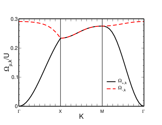
Figure 4: (Color online) Dispersion relation (65) of the elementary excitations of the effective boson model (58) along paths in the Brillouin zone [Fig. 1(c)] at the harmonic approximation. Such a spectrum corresponds to the spin wave excitations of the flat-band ferromagnetic phase of the Chern insulator (53).

IV Ferromagnetism in a flat-band Z₂ topological insulator

In this section, we study the flat-band ferromagnetic phase of a topological Hubbard model that preserves time-reversal symmetry. Due to the similarities with Sec. III, here we just quote the main results and comment on the differences between flat-band Chern and topological insulators.

IV.1 Time-reversal symmetric square lattice $\pi$-flux model

Similar to Sec. III.1, we consider $N$ spinfull noninteracting electrons hopping on a bipartite square lattice where each sublattice, $A$ and $B$, has $N_{A}=N_{B}=N$ sites. The Hamiltonian of the system $\mathcal{H}^{TRS}_{0}$ is given by Eq. (1) but now we assume that $\gamma(\uparrow)=-\gamma(\downarrow)=1$ for the nearest-neighbor hopping energy (2). Such a choice implies that time-reversal symmetry is preserved, see Appendix A for details. $\mathcal{H}^{TRS}_{0}$ can be seen as two copies of the spinless $\pi$-flux modelneupert11 where electrons with spin $\uparrow$ and $\downarrow$ are in the presence of opposite (fictitious) staggered $\pm\pi$ flux patterns, see Fig. 1(a).

In momentum space, $\mathcal{H}^{TRS}_{0}$ assumes the form (7) but with $h^{\downarrow}_{\bf k}=h^{\uparrow\;*}_{-{\bf k}}$, which is precisely a consequence of invariance under time-reversal transformations. It is easy to see that $\mathcal{H}^{TRS}_{0}$ can be diagonalized by the the Bogoliubov transformation

$$c^{\dagger}_{{\bf k}\,A\,\uparrow} = u_{\bf k}d^{\dagger}_{{\bf k}\,\uparrow}+v^{*}_{\bf k}c^{\dagger}_{{\bf k}\,\uparrow},\;\;\;\;\;\;c^{\dagger}_{{\bf k}\,B\,\uparrow}=v_{\bf k}d^{\dagger}_{{\bf k}\,\uparrow}-u^{*}_{\bf k}c_{{\bf k}\,\uparrow},$$

$$c^{\dagger}_{{\bf k}\,A\,\downarrow} = u^{*}_{-{\bf k}}d^{\dagger}_{{\bf k}\,\downarrow}+v_{-{\bf k}}c^{\dagger}_{{\bf k}\,\downarrow},\;\;\;c^{\dagger}_{{\bf k}\,B\,\downarrow}=v^{*}_{-{\bf k}}d^{\dagger}_{{\bf k}\,\downarrow}-u_{-{\bf k}}c^{\dagger}_{{\bf k}\,\downarrow},$$

with the Bogoliubov coefficients $u_{{\bf k}}$ and $v_{{\bf k}}$ given by Eq. (87). Note that since $h^{\downarrow}_{\bf k}=h^{\uparrow\;*}_{-{\bf k}}$, the canonical transformation for spin $\uparrow$ electrons differs from the one for spin $\downarrow$ electrons in contrast to the Chern insulator discussed in Sec. III.1, where both transformations are equal [see Eq. (17)]. After diagonalization, the Hamiltonian also assumes the form (18), but now the $4\times 4$ matrix $\mathcal{H^{\prime}}_{\bf k}$ reads

$$\mathcal{H^{\prime}}_{\bf k}=\left(\begin{array}[]{cc}h^{\prime}_{\bf k}&0\\ 0&h^{\prime}_{-{\bf k}}\end{array}\right)$$ (68)

with the $2\times 2$ diagonal matrix $h^{\prime}_{\bf k}$ giving by Eq. (20). Similarly to the Chern insulator discussed in Sec. III.1, the resulting band structure comprises two doubly degenerate bands $c$ and $d$, whose dispersion relations $\omega_{c/d,\sigma,{\bf k}}$ are also given by Eq. (21) [see Fig. 2]. As required by time-reversal symmetry,goerbig12 $\omega_{c/d,\sigma,{\bf k}}=\omega_{c/d,-\sigma,-{\bf k}}$. In particular, for the $\pi$-flux model $\mathcal{H}^{TRS}_{0}$, $\omega_{c/d,\uparrow,{\bf k}}=\omega_{c/d,\downarrow,{\bf k}}$.

Again, the $c$ and $d$ bands are topologically nontrivial. Indeed, it follows from Eq. (23) in combination with the fact that $\gamma(\uparrow)=-\gamma(\downarrow)=1$ that the Chern numbers of the $c$ and $d$ bands are given byneupert12

$$C^{d}_{\uparrow}=-C^{d}_{\downarrow}=-1\;\;\;\;\;\;\;{\rm and}\;\;\;\;\;\;\;C^{c}_{\uparrow}=-C^{c}_{\downarrow}=+1,$$

i.e., $C^{c/d}_{\sigma}=-C^{c/d}_{-\sigma}$ as required by time–reversal symmetry. As a consequence, the charge Chern numbersneupert12 of the $c$ and $d$ bands vanish,

$$C^{c/d}_{c}=\frac{1}{2}\left(C^{c/d}_{\uparrow}+C^{c/d}_{\downarrow}\right)=0,$$

while the corresponding spin Chern numbers are nonzero,

$$C^{c/d}_{s}=\frac{1}{2}\left(C^{c/d}_{\uparrow}-C^{c/d}_{\downarrow}\right)=\pm 1.$$

Since $\mathcal{H}^{TRS}_{0}$ conserves the $\hat{z}$-component of the total spin (see Sec. II.1), the Z₂ topological invariant for the $c$ and $d$ bands are simply given bykane13 ; sheng06

$$\nu_{c/d}=C^{c/d}_{s}\;{\rm mod}\;2=1,$$ (69)

implying that $\mathcal{H}^{TRS}_{0}$ is a Z₂ topological insulator. Indeed, at half-filling (configuration not considered here), $\mathcal{H}^{TRS}_{0}$ should display a QSHE with the spin Hall conductivity $\sigma^{SH}_{xy}=eC_{s}/2\pi$.

IV.2 Bosonization scheme for a flat-band topological insulator

In this section, we introduce a bosonization scheme for a flat-band Z₂ topological insulator similar to the one for the flat-band Chern insulator discussed in Sec. III.2. As shown below, the two bosonization schemes are quite similar, but there are important differences due to the fact that here time-reversal symmetry is preserved. Again, we focus on the nearly flat-band limit of the tight-binding model $\mathcal{H}^{TRS}_{0}$ ($t_{2}=t_{1}/\sqrt{2}$) at $1/4$-filling ($N_{A}=N_{B}=N$). We restrict the Hilbert space to the lowest energy $c$ bands and also assume that the ground state of $\mathcal{H}^{TRS}_{0}$ is given by the ferromagnet state (24).

Instead of the spin operator (25) at site $i$ of the sublattice $a$, we now consider the following spin operator

$${\bf S}_{i\,ab}=\frac{1}{2}c^{\dagger}_{i\,a\,\sigma}\hat{\sigma}_{\sigma\,\sigma^{\prime}}c_{i\,b\,\sigma^{\prime}}$$ (70)

with $(a,b)=(A,B)$ and $(B,A)$. Using Eqs. (6) and (26), the expression of the spin operators (70) in momentum space can be derived. In particular,

$$S^{+}_{{\bf q},ab} = \sum_{\bf p}c^{\dagger}_{{\bf p}-{\bf q}\,a\,\uparrow}c_{{\bf p}\,b\,\downarrow},$$

$$S^{-}_{{\bf q},ab} = \sum_{\bf p}c^{\dagger}_{{\bf p}-{\bf q}\,a\,\downarrow}c_{{\bf p}\,b\,\uparrow},$$ (71)

where $S^{\pm}_{{\bf q},ab}=S^{x}_{{\bf q},ab}\pm iS^{y}_{{\bf q},ab}$. The spin operators $\bar{S}^{\pm}_{{\bf q},ab}$ projected into the $c$ bands, i.e., the equivalent of Eq. (29), now read

$$\bar{S}^{+}_{{\bf q},ab} = \sum_{\bf p}G^{*}_{ab}(-{\bf p},-{\bf q})c^{\dagger}_{{\bf p}-{\bf q}\,\uparrow}c_{{\bf p}\,\downarrow},$$

$$\bar{S}^{-}_{{\bf q},ab} = \sum_{\bf p}G_{ab}({\bf p},{\bf q})c^{\dagger}_{{\bf p}-{\bf q}\,\downarrow}c_{{\bf p}\,\uparrow},$$ (72)

where

$$G_{AB}({\bf p},{\bf q})=-v_{-{\bf p}+{\bf q}}u_{\bf p}\;\;\;\;{\rm and}\;\;\;\;G_{BA}({\bf p},{\bf q})=-u_{-{\bf p}+{\bf q}}v_{\bf p}.$$

Again, we consider the following linear combination of the spin operators

$$\bar{S}^{\lambda}_{{\bf q},\alpha}=\bar{S}^{\lambda}_{{\bf q},AB}+(-1)^{\alpha}\bar{S}^{\lambda}_{{\bf q},BA}$$ (73)

with $\lambda=x,y,z$ and $\alpha=0,1$. In particular, we have

$$\bar{S}^{+}_{{\bf q},\alpha} = \sum_{\bf p}g^{*}_{\alpha}(-{\bf p},-{\bf q})c^{\dagger}_{{\bf p}-{\bf q}\,\uparrow}c_{{\bf p}\,\downarrow},$$

$$\bar{S}^{-}_{{\bf q},\alpha} = \sum_{\bf p}g_{\alpha}({\bf p},{\bf q})c^{\dagger}_{{\bf p}-{\bf q}\,\downarrow}c_{{\bf p}\,\uparrow},$$ (74)

where the $g_{\alpha}({\bf p},{\bf q})$ functions are now defined by

$$g_{\alpha}({\bf p},{\bf q})=-v_{-{\bf p}+{\bf q}}u_{\bf p}-(-1)^{\alpha}u_{-{\bf p}+{\bf q}}v_{\bf p}$$ (75)

with $\alpha=0,1$ [compare Eqs. (33) and (75)].

Similar to the flat-band Chern insulators, the algebra of the projected spin and electron density operators is not closed. For instance, the equivalent of the commutator (38) now reads

$$[\bar{S}^{+}_{{\bf q},\alpha},\bar{S}^{-}_{{\bf q}^{\prime},\beta}] = \sum_{\bf p}\left[g^{*}_{\alpha}(-{\bf p}+{\bf q}^{\prime},-{\bf q})g_{\beta}({\bf p},{\bf q}^{\prime})c^{\dagger}_{{\bf p}-{\bf q}-{\bf q}^{\prime}\,\uparrow}c_{{\bf p}\,\uparrow}\right.$$ (76)

$$- \left.g^{*}_{\alpha}(-{\bf p},-{\bf q})g_{\beta}({\bf p}-{\bf q},{\bf q}^{\prime})c^{\dagger}_{{\bf p}-{\bf q}-{\bf q}^{\prime}\,\downarrow}c_{{\bf p}\,\downarrow}\right].\;$$

The complete algebra of the projected spin and electron density operators can be found in Appendix C.

The construction of the boson operators $b_{\alpha}$ in terms of the fermion operators $c$ follows the same procedure outlined in Eqs. (39)–(43). Importantly, the spin operator that defines the particle-hole excitation [Eq. (39)] is now given by Eq. (73). Again, we can define two sets of independent boson operators, namely

$$b_{\alpha,{\bf q}} = \frac{1}{F_{\alpha,{\bf q}}}\sum_{\bf p}g^{*}_{\alpha}(-{\bf p},{\bf q})c^{\dagger}_{{\bf p}+{\bf q}\,\uparrow}c_{{\bf q}\,\downarrow},$$

$$b^{\dagger}_{\alpha,{\bf q}} = \frac{1}{F_{\alpha,{\bf q}}}\sum_{\bf p}g_{\alpha}({\bf p},{\bf q})c^{\dagger}_{{\bf p}-{\bf q}\,\downarrow}c_{{\bf q}\,\uparrow},$$ (77)

with $\alpha=0,1$, that obey the commutation relations (44). Here, the $g_{\alpha}({\bf p},{\bf q})$ functions are given by Eq. (75) and

$$F^{2}_{\alpha,{\bf q}} = \sum_{\bf p}g^{*}_{\alpha}(-{\bf p}+{\bf q},{\bf q})g_{\alpha}({\bf p},{\bf q})$$ (78)

[see Eq (101) for the expression of the $F_{\alpha,{\bf q}}$ function in terms of the coefficients $\hat{B}_{i,{\bf p}}$]. It is worth mentioning that although for both Chern and Z₂ topological insulators the bosons $b_{\alpha}$ are linear combinations of particle-hole pair excitations, for the former the particle and the hole are on the same sublattice [see Eqs. (31) and (43)] while, for the latter, the particle and the hole are on different sublattices [see Eqs. (73) and (77)].kumar14

Finally, the electron density operator (36) projected into the $c$ bands [the equivalent of Eq. (37)] now reads

$$\bar{\rho}_{a\,\sigma}({\bf k})=\sum_{\bf p}G_{a\,\sigma}({\bf p},{\bf k})c^{\dagger}_{{\bf p}-{\bf k}\,\sigma}c_{{\bf p}\,\sigma}$$ (79)

with

$$G_{A\,\uparrow}({\bf p},{\bf k}) = v^{*}_{{\bf p}-{\bf k}}v_{\bf p},\;\;\;\;\;\;\;\;G_{B\,\uparrow}({\bf p},{\bf k})=u^{*}_{{\bf p}-{\bf k}}u_{\bf p},$$

$$G_{A\,\downarrow}({\bf p},{\bf k}) = v_{-{\bf p}+{\bf k}}v^{*}_{-{\bf p}},\;\;\;\;G_{B\,\downarrow}({\bf p},{\bf k})=u_{-{\bf p}+{\bf k}}u^{*}_{-{\bf p}}.$$

Following the procedure outlined in Eqs. (46)–(52), the bosonic representation of (79) can be easily derived. It is also given by Eq. (52) but with the $\mathcal{G}_{\alpha\beta\,a\,\sigma}(x,y)$ function now given by Eq. (LABEL:galphabeta-shall01). Here, the equivalent of Eq. (51) reads

$$H_{\alpha}({\bf q},{\bf p},{\bf q})=\frac{1}{F_{\alpha,{\bf q}}}g^{*}_{\alpha}(-{\bf p}+{\bf q},{\bf q}).$$ (81)

IV.3 Topological Hubbard model II

In this section, we consider a correlated topological insulator on a square lattice described by the Hamiltonian

$$\mathcal{H}_{Z2}=\mathcal{H}^{TRS}_{0}+\mathcal{H}_{U},$$ (82)

where $\mathcal{H}^{TRS}_{0}$ is the square lattice $\pi$-flux model discussed in Sec. IV.1 in the nearly flat-band limit ($t_{2}=t_{1}/\sqrt{2}$) and $\mathcal{H}_{U}$ is the repulsive on-site Hubbard term (54). Again, $1/4$-filling is assumed. The topological Hubbard model (82) has recently been discussed by Neupert et al.neupert12 Similarly to Sec III.2, we now apply the bosonization formalism introduced in Sec. IV.2 to study the flat-band ferromagnetic phase of the Hamiltonian (82).

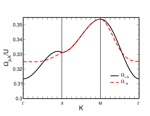
Figure 5: (Color online) Dispersion relation (83) of the elementary excitations of the effective boson model $\mathcal{H}^{Z2}_{B}$ along paths in the Brillouin zone [Fig. 1(c)] at the harmonic approximation. Such a spectrum corresponds to the spin wave excitations of the flat-band ferromagnetic phase of the Z₂ topological insulator (82).

Following the lines of Sec. III.3, the first step is to project the Hamiltonian (82) into the lowest-energy $c$ bands, i.e,

$$\mathcal{H}_{Z2}\rightarrow\mathcal{\bar{H}}_{Z2}.$$

We then map the projected Hubbard model $\mathcal{\bar{H}}_{Z2}$ to an effective interacting boson model $\mathcal{H}^{Z2}_{B}$. We find that $\mathcal{H}^{Z2}_{B}$ has the same form as the boson Hamiltonian (58) but with the $\mathcal{G}_{\alpha\beta\,a\,\sigma}(x,y)$ function given by Eq. (LABEL:galphabeta-shall01).

Within the harmonic approximation, the effective boson model $\mathcal{H}^{Z2}_{B}$ can be diagonalized and it assumes the form (64). The dispersion relation of the bosons $a_{\pm}$ is equal to (65), i.e.,

$$\Omega^{Z2}_{\pm,{\bf p}}=\pm\Delta_{\bf p}+\sqrt{\epsilon^{2}_{\bf p}-\epsilon^{10}_{\bf p}\epsilon^{01}_{\bf p}}$$ (83)

but with the $\mathcal{G}_{\alpha\beta\,a\,\sigma}(x,y)$ function given by Eq. (LABEL:galphabeta-shall01).

Similarly to the correlated Chern insulator discussed in Sec. III.3, the ground state of $\mathcal{H}^{Z2}_{B}$ is the vacuum state for the bosons $a_{\pm}$, i.e., the ferromagnetic state $|{\rm FM}\rangle$ [Eq. (24)], and the excitation spectrum [the dispersion relation (83) of the bosons $a_{\pm}$] of such a flat-band ferromagnet has two branches, see Fig. 5. However, in contrast to the spin-wave spectrum of a Chern insulator (Fig. 4), here both branches are gapped at zero wave vector. Differently from the flat-band Chern insulator (53), where a continuous SU(2) symmetry is broken, the ground state of the correlated topological insulator preserves the U(1) spin rotation symmetry of the Hamiltonian (82) (see Sec. II.1 for more details). As a consequence, a Goldstone mode is absent in the excitation spectrum. Again, the energy scale of the spin-wave excitations is given by the on-site repulsion energy $U$. The excitation gap $\Delta=\Omega^{Z2}_{+,{\bf k}=0}=0.3134\,U$, which is at the centre of the Brillouin zone, agrees with the exact diagonalization data from Neupert et al., $\Delta\approx 0.30\,U$.neupert12 The fact that the spin-wave excitations remain gapped at all wave vectors corroborates that the ground state is indeed given by our reference state (24) and not by an in-plane ($XY$-type) ferromagnetic state.

Interestingly, since a phase with ferromagnetic long-range order sets in, time-reversal symmetry is spontaneously broken. As shown in Ref. neupert12, , the ferromagnet ground state also displays an IQHE with the Hall conductivity $\sigma_{xy}=e^{2}/h$.

V Discussion

Although we have focused our discussion on the square lattice $\pi$-flux model, the bosonization formalisms for flat-band Chern and topological insulators, respectively introduced in Secs. III.2 and IV.2, are rather general. In principle, they can be employed to study the flat-band ferromagnetic phase of a topological Hubbard model whose single-particle term assumes the $4\times 4$ matrix form (7), such as the Kane-Mele-Hubbard model without the Rashba spin-orbit coupling.assaad13 In this case, spin is a good quantum number. Once the coefficients $B_{i,{\bf k}}$ [Eq. (11)] of the model are identified, the corresponding effective (interacting) boson model is easily determined since the coefficients (61) and (62) of the boson model are written in terms of the $\hat{{\bf B}}_{i,{\bf k}}=B_{i,{\bf k}}/|{\bf B}_{\bf k}|$ functions (see Appendices B and C). One important point is to verify whether the condition (42) holds, i.e., if it is possible to define two sets of independent boson operators. It would be interesting to see whether the bosonization scheme could be extended to the following cases: (i) Four band models where spin is not conserved. It would allow us to consider, e. g., the Kane-Mele-Hubbard model with a Rashba coupling.assaad13 (ii) Six band models where the single-particle term assumes the form (7) but with $h^{\sigma}_{\bf k}$ being a $3\times 3$ matrix. Two examples are the tight-binding model on the kagome latticetang11 and the three-orbital square lattice model.sun11

One interesting feature of the bosonization scheme developed here is that it allows us to analytically determine the spin-wave excitation spectrum of a flat-band ferromagnet with topologically nontrivial single-particle bands. At the moment, it is not clear how to compare the results derived in Secs. III.3 and IV.3 with other approximation schemes. For the 2DEG at filling factor $\nu=1$, the noninteracting term of the effective boson model derived within the bosonization formalismdoretto05 describes the magnetic exciton excitations of the quantum Hall ferromagnetic ground state. The energy of the bosons are exactly equal to the magnetic exciton dispersion relation derived by Kallin and Halperinkallin84 within diagrammatic calculations. Such a diagrammatic formalism is indeed equivalent to the so-called time-dependent Hartree-Fock approximation.macdonald85 Although for flat-band Chern and topological insulators only an approximated bosonic representation for the electron density operator can be derived [Eq. (52)], we expected that, due to the analogy with the 2DEG at $\nu=1$ (see discussion at the end of Sec. III.2), the spin-wave dispersion relations determined in Secs. III.3 and IV.3 agree with a time-dependent Hartree-Fock analysis of the topological Hubbard models (53) and (82).

A second interesting aspect of the bosonization scheme for flat-band Chern and topological insulators is that it provides an interaction between the bosons (spin-waves). A detailed study of the consequences of the spin-wave–spin-wave coupling is beyond the scope of the present paper. It would be interesting, for instance, to verify whether the boson-boson interaction (60) yields two-spin-wave bound states and whether such bound states are related to possible topological excitations of the flat-band ferromagnetic state (24). Such an analysis is motivated by the fact that for the 2DEG at filling factor $\nu=1$, the boson-boson coupling derived within the bosonization formalismdoretto05 gives rise to two-boson bound states that are related to skyrmion-antiskyrmion pair excitations (the charged excitation of the 2DEG at $\nu=1$ is described as a topological excitation, quantum Hall skyrmion, of the quantum Hall ferromagnetic ground state). This set of results allows us to properly treat the skyrmion as an electron bound to a certain number of boson (spin-waves).doretto05-1 We defer the analysis of the effects of the boson-boson interacting (60) to a future publication.

VI Summary

In this paper, we have considered the flat-band ferromagnetic phase of a correlated Chern insulator and a correlated Z₂ topological insulator and analytically calculated the corresponding spin-wave excitation spectra. In particular, we have considered two variants of a topological Hubbard model, namely, one with broken time-reversal symmetry (Chern insulator) and another one invariant under time-reversal symmetry (topological insulator). In both cases, the single-particle term is the square lattice $\pi$-flux model with topologically nontrivial and nearly flat bands. The spin-wave dispersion relation has been determined within a bosonization scheme similar to the formalismdoretto05 previously developed for the 2DEG at filling factor $\nu=1$. Here, we showed that the formalismdoretto05 can indeed be generalized for flat-band Chern and topological insulators.

The investigation of the spin-wave excitation spectrum indicates the stability of the flat-band ferromagnetic phase. Generically, we obtain two spin-wave excitation branches due to the two-atom basis of the lattice model. We find that the correlated flat-band Chern insulator has a gapless excitation spectrum: the Goldstone mode is associated with a spontaneous SU(2) spin-symmetry breaking. For the correlated flat-band topological insulator with preserved time-reversal symmetry, the excitation spectrum is gapped since the flat-band ferromagnetic ground state preserves the U(1) spin rotation symmetry of the Hamiltonian. Moreover, within the bosonization scheme, we find a spin-wave-spin-wave interaction. Due to the analogies with the 2DEG at filling factor $\nu=1$, we expect that such coupling may give rise to two-spin-wave bound states.

Appendix A Symmetries of the $\pi$-flux model: time-reversal

In this section, we discuss the behavior of the noninteracting fermion model (1) under time-reversal.

The time-reversal operator $\mathcal{T}$ is defined as

$$\mathcal{T}=i\left(\sigma_{y}\otimes I\right)K,$$ (84)

where $K$ denotes complex conjugation and $I$ is the $2\times 2$ identity matrix. Invariance under time reversal, i.e., $[\mathcal{H}_{0},\mathcal{T}]=0$, implies thatfu07

$$\mathcal{T}\mathcal{H}_{\bf k}\mathcal{T}^{-1}=\mathcal{H}_{-{\bf k}},$$

where $\mathcal{H}_{\bf k}$ is the matrix (8). Since

$$\mathcal{T}\mathcal{H}_{\bf k}\mathcal{T}^{-1}=\left(\begin{array}[]{cc}h^{\downarrow\,*}_{\bf k}&0\\ 0&h^{\uparrow\,*}_{\bf k}\end{array}\right),$$

invariance under time-reversal implies that $h^{\downarrow}_{\bf k}=h^{\uparrow\,*}_{-{\bf k}}$ as mentioned in Sec. II.

Alternatively, we can follow Lu and Kanefu07 and write the matrix $\mathcal{H}_{\bf k}$ in terms of the five $4\times 4$ Dirac matrices

$$\Gamma^{1,2,3,4,5}=\left(I\,\otimes\,\tau_{x},I\,\otimes\,\tau_{y},\sigma_{x}\,\otimes\,\tau_{z},\sigma_{y}\,\otimes\,\tau_{z},\sigma_{z}\,\otimes\,\tau_{z}\right),$$

and their ten commutators $\Gamma^{ij}=[\Gamma^{i},\Gamma^{j}]/(2i).$ Here, $\sigma_{x,y,z}$ and $\tau_{x,y,z}$ are $2\times 2$ Pauli matrices respectively related to spin and sublattice. The Dirac matrices obey the Clifford algebra $\Gamma^{i}\Gamma^{j}+\Gamma^{i}\Gamma^{j}=2\delta_{ij}I.$ For the Chern insulator discussed in Secs. II and III.1,

$$\mathcal{H}_{\bf k}=B_{1,{\bf k}}\Gamma^{1}+B_{2,{\bf k}}\Gamma^{2}+B_{3,{\bf k}}\Gamma^{12}$$ (85)

while, for the topological insulator considered in Secs. II and IV.1,

$$\mathcal{H}_{\bf k}=B_{1,{\bf k}}\Gamma^{1}+B_{2,{\bf k}}\Gamma^{51}+B_{3,{\bf k}}\Gamma^{12}.$$ (86)

Since $B_{i,{\bf k}}=B_{i,-{\bf k}}$,

$$\mathcal{T}\Gamma^{i}\mathcal{T}^{-1}=\left\{\begin{array}[]{cl}+\Gamma^{1},&i=1,\\ -\Gamma^{i},&i=2,3,4,5,\end{array}\right.$$

$\mathcal{T}\Gamma^{12}\mathcal{T}^{-1}=\Gamma^{12}$, and $\mathcal{T}\Gamma^{51}\mathcal{T}^{-1}=\Gamma^{51}$, we see that only the Hamiltonian (86) is invariant under time-reversal.

Appendix B Details of the bosonization scheme for flat-band Chern insulators

In this section, we quote the expressions in terms of the coefficients $B_{i,{\bf k}}$ of some quantities related to the bosonization scheme discussed in Sec. III.

Let us first consider the diagonalization of the noninteracting Hamiltonian (7). It is useful to write the coefficients $u_{\bf k}$ and $v_{\bf k}$ of the Bogoliubov transformation (17) as

$$u_{\bf k} = \exp(+i\phi_{\bf k}/2)\cos(\theta_{\bf k}/2),$$

$$v_{\bf k} = \exp(-i\phi_{\bf k}/2)\sin(\theta_{\bf k}/2).$$ (87)

Due to the form of the matrix $h^{\uparrow}_{\bf k}$ [see Eq. (10)], it is interesting to introduce the following relations between the $\phi_{\bf k}$ and $\theta_{\bf k}$ functions and the coefficients $B_{i,{\bf k}}$ [Eq. (11)]:

$$\hat{B}_{1,{\bf k}} = \sin\theta_{\bf k}\cos\phi_{\bf k},\;\;\;\;\;\;\;\;\;\;\;\hat{B}_{2,{\bf k}}=\sin\theta_{\bf k}\sin\phi_{\bf k},$$

$$\hat{B}_{3,{\bf k}} = \cos\theta_{\bf k},$$

$$\sin\theta_{\bf k} = \sqrt{\hat{B}^{2}_{1,{\bf k}}+\hat{B}^{2}_{2,{\bf k}}},\;\;\;\;\;\tan\phi_{\bf k}=\frac{\hat{B}_{2,{\bf k}}}{\hat{B}_{1,{\bf k}}},$$ (88)

where $\hat{{\bf B}}_{\bf k}\equiv{\bf B}_{\bf k}/|{\bf B}_{\bf k}|$. It then follows that

$$|u_{\bf k}|^{2} = \frac{1}{2}\left(1+\hat{B}_{3,{\bf k}}\right),\;\;\;\;\;\;\;|v_{\bf k}|^{2}=\frac{1}{2}\left(1-\hat{B}_{3,{\bf k}}\right),$$

$$u^{*}_{\bf k}v_{\bf k} = \frac{1}{2}\left(\hat{B}_{1,{\bf k}}+i\hat{B}_{2,{\bf k}}\right).$$ (89)

With the aid of Eqs. (87)-(89), it is easy to show that the Hamiltonian (18) is the diagonal form of (7).

Concerning the algebra of the projected spin and electron density operators, in addition to the commutator (38), it follows from Eqs. (32) and (37) that

$$[\bar{\rho}_{a\,\sigma}({\bf k}),\bar{S}^{+}_{{\bf q},\alpha}] = \sum_{\bf p}\left[\delta_{\sigma,\uparrow}G_{a}({\bf p}-{\bf q},{\bf k})g_{\alpha}({\bf p},{\bf q})-\delta_{\sigma,\downarrow}G_{a}({\bf p},{\bf k})g_{\alpha}({\bf p}-{\bf k},{\bf q})\right]c^{\dagger}_{{\bf p}-{\bf q}-{\bf k}\,\uparrow}c_{{\bf p}\,\downarrow},$$ (90)

$$\,[\bar{\rho}_{a\,\sigma}({\bf k}),\bar{S}^{-}_{{\bf q},\alpha}] = \sum_{\bf p}\left[\delta_{\sigma,\downarrow}G_{a}({\bf p}-{\bf q},{\bf k})g_{\alpha}({\bf p},{\bf q})-\delta_{\sigma,\uparrow}G_{a}({\bf p},{\bf k})g_{\alpha}({\bf p}-{\bf k},{\bf q})\right]c^{\dagger}_{{\bf p}-{\bf q}-{\bf k}\,\downarrow}c_{{\bf p}\,\uparrow},$$ (91)

$$\,[\bar{\rho}_{a\,\sigma}({\bf k}),\bar{\rho}_{b\,\sigma^{\prime}}({\bf q})] = \delta_{\sigma,\sigma^{\prime}}\sum_{\bf p}\left[G_{a}({\bf p}-{\bf q},{\bf k})G_{b}({\bf p},{\bf q})-G_{a}({\bf p},{\bf k})G_{b}({\bf p}-{\bf k},{\bf q})\right]c^{\dagger}_{{\bf p}-{\bf q}-{\bf k}\,\sigma}c_{{\bf p}\,\sigma},$$ (92)

with $a,b=A,B$, $\alpha=0,1$, and the $G_{a}({\bf p},{\bf q})$ and $g_{\alpha}({\bf p},{\bf q})$ functions respectively given by Eqs. (30) and (33).

Within the approximation (40), the commutator (38) assumes the form (42). With the aid of Eq. (89), it is possible to show that ($\alpha\not=\beta$)

$$\sum_{\bf p}g_{\alpha}({\bf p},{\bf q})g_{\beta}({\bf p}-{\bf q},-{\bf q})=\frac{1}{2}\sum_{\bf p}\left[(-1)\left(\hat{B}_{3,{\bf p}}+\hat{B}_{3,{\bf p}-{\bf q}}\right)+i(-1)^{\alpha}\left(\hat{B}_{1,{\bf p}-{\bf q}}\hat{B}_{2,{\bf p}}-\hat{B}_{2,{\bf p}-{\bf q}}\hat{B}_{1,{\bf p}}\right)\right].$$ (93)

Since for the $\pi$-flux model, $B_{i,{\bf k}}=B_{i,-{\bf k}}$ [see Eq. (11)] it is then easy to show that Eq. (93) vanishes.

Similar to Eq. (93), it is possible to write the $F_{\alpha,{\bf q}}$ function in terms of the coefficients $B_{i,{\bf k}}$. Using Eq. (89), we show that

$$F^{2}_{\alpha,{\bf q}}=\frac{1}{2}\sum_{\bf p}\left[1+\hat{B}_{3,{\bf p}}\hat{B}_{3,{\bf p}-{\bf q}}(-1)^{\alpha}\left(\hat{B}_{1,{\bf p}}\hat{B}_{1,{\bf p}-{\bf q}}+\hat{B}_{2,{\bf p}}\hat{B}_{2,{\bf p}-{\bf q}}\right)\right].$$ (94)

The (approximated) boson representation of the projected electron-density operator is given by Eq. (52) where the $\mathcal{G}_{\alpha\,\beta\,a\,\alpha}({\bf k},{\bf q})$ function is defined as

$$\mathcal{G}_{\alpha\,\beta\,a\,\uparrow}({\bf k},{\bf q}) = -\frac{1}{F_{\alpha,{\bf q}}F_{\beta,{\bf k}+{\bf q}}}\sum_{\bf p}G_{a}({\bf p},{\bf k})g_{\alpha}({\bf p}-{\bf k},{\bf q})g_{\beta}({\bf p}-{\bf k}-{\bf q},-{\bf k}-{\bf q}),$$

$$\mathcal{G}_{\alpha\,\beta\,a\,\downarrow}({\bf k},{\bf q}) = +\frac{1}{F_{\alpha,{\bf q}}F_{\beta,{\bf k}+{\bf q}}}\sum_{\bf p}G_{a}({\bf p}-{\bf q},{\bf k})g_{\alpha}({\bf p},{\bf q})g_{\beta}({\bf p}-{\bf k}-{\bf q},-{\bf k}-{\bf q}).$$

Again, using Eqs. (89), we find after some algebra that

$$\mathcal{G}_{\alpha\,\beta\,a\,\uparrow}({\bf k},{\bf q})=-\frac{1}{8}[\delta_{a,A}+\delta_{a,B}(-1)^{\alpha+\beta}]\frac{1}{F_{\alpha,{\bf q}}F_{\beta,{\bf k}+{\bf q}}}\sum_{\bf p}1-3(-1)^{a}\hat{B}_{3,{\bf p}}$$

$$\;+\hat{B}_{3,{\bf p}-{\bf q}}\hat{B}_{3,{\bf p}+{\bf k}}+\hat{B}_{3,{\bf p}-{\bf q}}\hat{B}_{3,{\bf p}}+\hat{B}_{3,{\bf p}+{\bf k}}\hat{B}_{3,{\bf p}}-(-1)^{a}\hat{B}_{3,{\bf p}-{\bf q}}\hat{B}_{3,{\bf p}}\hat{B}_{3,{\bf p}+{\bf k}}$$

$$\;+(-1)^{\alpha}[\hat{B}_{1,{\bf p}-{\bf q}}\hat{B}_{1,{\bf p}}+\hat{B}_{2,{\bf p}-{\bf q}}\hat{B}_{2,{\bf p}}+i(-1)^{a}(\hat{B}_{1,{\bf p}-{\bf q}}\hat{B}_{2,{\bf p}}-\hat{B}_{2,{\bf p}-{\bf q}}\hat{B}_{1,{\bf p}})][1-(-1)^{a}\hat{B}_{3,{\bf p}+{\bf k}}]$$

$$\;+(-1)^{\beta}[\hat{B}_{1,{\bf p}-{\bf q}}\hat{B}_{1,{\bf p}+{\bf k}}+\hat{B}_{2,{\bf p}-{\bf q}}\hat{B}_{2,{\bf p}+{\bf k}}-i(-1)^{a}(\hat{B}_{1,{\bf p}-{\bf q}}\hat{B}_{2,{\bf p}+{\bf k}}-\hat{B}_{2,{\bf p}-{\bf q}}\hat{B}_{1,{\bf p}+{\bf k}})][1-(-1)^{a}\hat{B}_{3,{\bf p}}]$$

$$\;+(-1)^{\alpha+\beta}[\hat{B}_{1,{\bf p}+{\bf k}}\hat{B}_{1,{\bf p}}+\hat{B}_{2,{\bf p}+{\bf k}}\hat{B}_{2,{\bf p}}+i(-1)^{a}(\hat{B}_{1,{\bf p}+{\bf k}}\hat{B}_{2,{\bf p}}-\hat{B}_{2,{\bf p}+{\bf k}}\hat{B}_{1,{\bf p}})][1+(-1)^{a}\hat{B}_{3,{\bf p}-{\bf q}}].$$ (96)

The expression of $\mathcal{G}_{\alpha\,\beta\,a\,\downarrow}({\bf k},{\bf q})$ can be derived from Eq. (96) using the fact that $\mathcal{G}_{\alpha\,\beta\,a\,\downarrow}({\bf k},{\bf q})=-\mathcal{G}^{*}_{\alpha\,\beta\,a\,\uparrow}(-{\bf k},-{\bf q})$.

Finally, the bosonic representation of the projected single-particle Hamiltonian (57). The first step is the calculation of the commutator

$$[\bar{\mathcal{H}}_{0},b^{\dagger}_{\alpha,{\bf q}}] = \sum_{\bf p}\left(\omega_{c,{\bf p}-{\bf q}}-\omega_{c,{\bf p}}\right)\frac{g_{\alpha}({\bf p},{\bf q})}{F_{\alpha,{\bf q}}}c_{{\bf p}-{\bf q}\,\downarrow}c_{{\bf p}\,\uparrow}=\sum_{\beta,{\bf k},{\bf p}}\left(\omega_{c,{\bf p}-{\bf q}}-\omega_{c,{\bf p}}\right)\frac{g_{\alpha}({\bf p},{\bf q})}{F_{\alpha,{\bf q}}}H_{\beta}({\bf k},{\bf p},{\bf q})b^{\dagger}_{\beta,{\bf k}}.$$ (97)

Here, the second equality follows from Eq. (47). Note that the expansion

$$\bar{\mathcal{H}}_{0,B}=\sum_{\alpha,\beta}\sum_{{\bf k},{\bf p},{\bf q}}\left(\omega_{c,{\bf p}-{\bf q}}-\omega_{c,{\bf p}}\right)\frac{g_{\alpha}({\bf p},{\bf q})}{F_{\alpha,{\bf q}}}H_{\beta}({\bf k},{\bf p},{\bf q})b^{\dagger}_{\beta,{\bf k}}b_{\alpha,{\bf k}}$$ (98)

of $\bar{\mathcal{H}}_{0}$ in terms of the boson operators $b_{\alpha}$ satisfies the commutator (97). Keeping only the term ${\bf k}={\bf q}$ in the momentum sum above and using Eq. (51), we have

$$\bar{\mathcal{H}}_{0,B}=E_{0}+\sum_{\alpha,\beta}\sum_{\bf q}\bar{\omega}_{\alpha\beta}({\bf q})b^{\dagger}_{\beta,{\bf q}}b_{\alpha,{\bf q}},$$ (99)

where $E_{0}=2.44N$ is a constant related to the action of $\bar{\mathcal{H}}_{0}$ in the reference state (24) and

$$\bar{\omega}_{\alpha\beta}({\bf q})=\frac{1}{F_{\alpha,{\bf q}}F_{\beta,{\bf q}}}\sum_{\bf p}\left(\omega_{c,{\bf p}-{\bf q}}-\omega_{c,{\bf p}}\right)g_{\alpha}({\bf p},{\bf q})g_{\beta}({\bf p}-{\bf q},-{\bf q}).$$ (100)

In the flat-band limit, $\bar{\omega}_{\alpha\beta}({\bf q})=0$ since $\omega_{c,{\bf p}}=0$. In the nearly flat-band limit considered in Sec. III.3, the coefficient $\bar{\omega}_{\alpha\beta}({\bf q})$ can be nonzero. However, for the $\pi$-flux model, it is possible to show that $\bar{\omega}_{\alpha\beta}({\bf q})$ vanishes due to the fact that $B_{i,{\bf k}}=B_{i,-{\bf k}}$.

Appendix C Details of the bosonization scheme for flat-band topological insulators

Similar to the previous section, we here provide the expansion in terms of the coefficients $B_{i,{\bf k}}$ of some functions related to the bosonization formalism introduced in Sec. IV.

The $F_{\alpha,{\bf q}}$ function (78) reads

$$F^{2}_{\alpha,{\bf q}}=\frac{1}{2}\sum_{\bf p}\left[(-1)^{\alpha}(1-\hat{B}_{3,{\bf p}}\hat{B}_{3,-{\bf p}+{\bf q}})+\hat{B}_{1,{\bf p}}\hat{B}_{1,-{\bf p}+{\bf q}}+\hat{B}_{2,{\bf p}}\hat{B}_{2,-{\bf p}+{\bf q}}\right].$$ (101)

The algebra of the projected spin and electron-density operators. From Eqs. (74) and (79), we show that, in addition to the commutator (76), the following commutation relations hold

$$[\bar{\rho}_{a\,\sigma}({\bf k}),\bar{S}^{+}_{{\bf q},\alpha}] = \sum_{\bf p}\left[\delta_{\sigma,\uparrow}G_{a\,\sigma}({\bf p}-{\bf q},{\bf k})g^{*}_{\alpha}(-{\bf p},-{\bf q})-\delta_{\sigma,\downarrow}G_{a\,\sigma}({\bf p},{\bf k})g^{*}_{\alpha}(-{\bf p}+{\bf k},-{\bf q})\right]c^{\dagger}_{{\bf p}-{\bf q}-{\bf k}\,\uparrow}c_{{\bf p}\,\downarrow},$$ (102)

$$\,[\bar{\rho}_{a\,\sigma}({\bf k}),\bar{S}^{-}_{{\bf q},\alpha}] = \sum_{\bf p}\left[\delta_{\sigma,\downarrow}G_{a\,\sigma}({\bf p}-{\bf q},{\bf k})g_{\alpha}({\bf p},{\bf q})-\delta_{\sigma,\uparrow}G_{a\,\sigma}({\bf p},{\bf k})g_{\alpha}({\bf p}-{\bf k},{\bf q})\right]c^{\dagger}_{{\bf p}-{\bf q}-{\bf k}\,\downarrow}c_{{\bf p}\,\uparrow},$$ (103)

$$\,[\bar{\rho}_{a\,\sigma}({\bf k}),\bar{\rho}_{b\,\sigma^{\prime}}({\bf q})] = \delta_{\sigma,\sigma^{\prime}}\sum_{\bf p}\left[G_{a\,\sigma}({\bf p}-{\bf q},{\bf k})G_{b\,\sigma^{\prime}}({\bf p},{\bf q})-G_{a\,\sigma}({\bf p},{\bf k})G_{b\,\sigma^{\prime}}({\bf p}-{\bf k},{\bf q})\right]c^{\dagger}_{{\bf p}-{\bf q}-{\bf k}\,\sigma}c_{{\bf p}\,\sigma},$$ (104)

with $a,b=A,B$, $\alpha=0,1$, and the $g_{\alpha}({\bf p},{\bf q})$ and $G_{a\,\sigma}({\bf p},{\bf q})$ functions respectively given by Eqs. (75) and (LABEL:gabsigma-functions).

The $\mathcal{G}_{\alpha\,\beta\,a\,\sigma}({\bf k},{\bf q})$ function, which is related to the bosonic representation of the projected electron-density operator (79), is defined as

$$\mathcal{G}_{\alpha\,\beta\,a\,\uparrow}({\bf k},{\bf q}) = -\frac{1}{F_{\alpha,{\bf q}}F_{\beta,{\bf k}+{\bf q}}}\sum_{\bf p}G_{a\,\uparrow}({\bf p},{\bf k})g_{\alpha}({\bf p}-{\bf k},{\bf q})g^{*}_{\beta}(-{\bf p}+{\bf k}+{\bf q},{\bf k}+{\bf q}),$$

$$\mathcal{G}_{\alpha\,\beta\,a\,\downarrow}({\bf k},{\bf q}) = +\frac{1}{F_{\alpha,{\bf q}}F_{\beta,{\bf k}+{\bf q}}}\sum_{\bf p}G_{a\,\downarrow}({\bf p}-{\bf q},{\bf k})g_{\alpha}({\bf p},{\bf q})g^{*}_{\beta}(-{\bf p}+{\bf k}+{\bf q},{\bf k}+{\bf q})$$

and, in terms of the coefficients $B_{i,{\bf q}}$, it reads

$$\mathcal{G}_{\alpha\,\beta\,a\,\uparrow}({\bf k},{\bf q})=-\frac{1}{8}[\delta_{a,A}+\delta_{a,B}(-1)^{\alpha+\beta}]\frac{1}{F_{\alpha,{\bf q}}F_{\beta,{\bf k}+{\bf q}}}\sum_{\bf p}(-1)^{\alpha}[1-(-1)^{a}\hat{B}_{3,{\bf p}}$$

$$\;-\hat{B}_{3,-{\bf p}+{\bf q}}\hat{B}_{3,{\bf p}+{\bf k}}-\hat{B}_{3,-{\bf p}+{\bf q}}\hat{B}_{3,{\bf p}}+\hat{B}_{3,{\bf p}+{\bf k}}\hat{B}_{3,{\bf p}}-(-1)^{a}\hat{B}_{3,-{\bf p}+{\bf q}}\hat{B}_{3,{\bf p}}\hat{B}_{3,{\bf p}+{\bf k}}]$$

$$\;+[\hat{B}_{1,-{\bf p}+{\bf q}}\hat{B}_{1,{\bf p}}+\hat{B}_{2,-{\bf p}+{\bf q}}\hat{B}_{2,{\bf p}}+i(-1)^{a}(\hat{B}_{1,-{\bf p}+{\bf q}}\hat{B}_{2,{\bf p}}-\hat{B}_{2,-{\bf p}+{\bf q}}\hat{B}_{1,{\bf p}})][1-(-1)^{a}\hat{B}_{3,{\bf p}+{\bf k}}]$$

$$\;+(-1)^{\alpha+\beta}[\hat{B}_{1,-{\bf p}+{\bf q}}\hat{B}_{1,{\bf p}+{\bf k}}+\hat{B}_{2,-{\bf p}+{\bf q}}\hat{B}_{2,{\bf p}+{\bf k}}-i(-1)^{a}(\hat{B}_{1,-{\bf p}+{\bf q}}\hat{B}_{2,{\bf p}+{\bf k}}-\hat{B}_{2,-{\bf p}+{\bf q}}\hat{B}_{1,{\bf p}+{\bf k}})][1-(-1)^{a}\hat{B}_{3,{\bf p}}]$$

$$\;+(-1)^{\beta}[\hat{B}_{1,{\bf p}+{\bf k}}\hat{B}_{1,{\bf p}}+\hat{B}_{2,{\bf p}+{\bf k}}\hat{B}_{2,{\bf p}}+i(-1)^{a}(\hat{B}_{1,{\bf p}+{\bf k}}\hat{B}_{2,{\bf p}}-\hat{B}_{2,{\bf p}+{\bf k}}\hat{B}_{1,{\bf p}})][1-(-1)^{a}\hat{B}_{3,-{\bf p}+{\bf q}}]$$ (106)

The expansion for $\mathcal{G}_{\alpha\,\beta\,a\,\downarrow}({\bf k},{\bf q})$ follows from Eq. (106) using the relation $\mathcal{G}_{\alpha\,\beta\,a\,\downarrow}({\bf k},{\bf q})=-(-1)^{\alpha+\beta}\mathcal{G}_{\alpha\,\beta\,a\,\uparrow}({\bf k},{\bf q})$.

References

- (1) M. Z. Hasan and C. L. Kane, Rev. Mod. Phys. 82, 3045 (2010).
- (2) C. L. Kane, in Topological Insulators, Contemporary Concepts of Condensed Matter Science Vol. 6, edited by M. Franz and L. Molenkamp (Elsevier, 2013), p. 3.
- (3) F. D. M. Haldane, Phys. Rev. Lett. 61, 2015 (1988).
- (4) C. L. Kane and E. J. Mele, Phys. Rev. Lett. 95, 146802 (2005)
- (5) C. L. Kane and E. J. Mele, Phys. Rev. Lett. 95, 226801 (2005).
- (6) B. A. Bernevig, T. L. Hughes, and S.-C. Zhang, Science 314, 1757 (2006).
- (7) M. König, S. Wiedmann, C. Brüne, A. Roth, H. Buhmann, L. W. Molenkamp, X. L. Qi, and S. C. Zhang, Science 318, 766 (2005).
- (8) E. Tang, J.-W. Mei, and X.-G. Wen, Phys. Rev. Lett. 106, 236802 (2011).
- (9) K. Sun, Z. Gu, H. Katsura, and S. Das Sarma, Phys. Rev. Lett. 106, 236803 (2011).
- (10) T. Neupert, L. Santos, C. Chamon, and C. Mudry, Phys. Rev. Lett. 106, 236804 (2011).
- (11) D. N. Sheng, Z.-C. Gu, K. Sun, and L. Sheng, Nature Commun. 2, 389 (2011).
- (12) N. Regnault and B. Andrei Bernevig, Phys. Rev. X 1, 021014 (2011).
- (13) S. A. Parameswaran, R. Roy, S. L. Sondhi, C. R. Phys. 14, 816 (2013).
- (14) E. J. Bergholtz and Z. Liu, Int. J. Mod. Phys. B 27, 1330017 (2013).
- (15) T. Neupert, C. Chamon, T. Iadecola, L. H. Santos, and C. Mudry, arXiv:1410.5828v1.
- (16) See, e.g., Z. F. Ezawa, Quantum Hall Effects: Recent Theoretical and Experimental Developments (World Scientific, 3 ed., 2013).
- (17) M. O. Goerbig, Eur. Phys. J. B 85, 14 (2012).
- (18) T. Neupert, L. Santos, S. Ryu, C. Chamon, and C. Mudry, Phys. Rev. Lett. 108, 046806 (2012).
- (19) R. L. Doretto, A. O. Caldeira, and S. M. Girvin, Phys. Rev. B 71, 045339 (2005).
- (20) R. L. Doretto and C. Morais Smith, Phys. Rev. B 76, 195431 (2007).
- (21) R. L. Doretto, A. O. Caldeira, and C. Morais Smith, Phys. Rev. Lett. 97, 186401 (2006).
- (22) R. L. Doretto, C. Morais Smith, and A. O. Caldeira, Phys. Rev. B 86, 035326 (2012)
- (23) For more details about the -flux model see, e.g., P. A. Lee, N. Nagaosa, and X.-G. Wen, Rev. Mod. Phys. 78, 17 (2006).
- (24) M. Hohenadler and F. F. Assaad, J. Phys.: Condens. Matter 25, 143201 (2013).
- (25) See, e.g., T. Giamarchi, Quantum Physics in One Dimension (Oxford University Press, 2004).
- (26) S. M. Girvin, A. H. MacDonald, and P. M. Platzman, Phys. Rev. B 33, 2481 (1986).
- (27) S. A. Parameswaran, R. Roy, and S. L. Sondhi, Phys. Rev. B 85, 241308(R) (2012).
- (28) R. Roy, Phys. Rev. B 90, 165139 (2014).
- (29) K. Kusakabe and H. Aoki, Phys. Rev. Lett. 72, 144 (1994).
- (30) Quantum Spin-Hall Effect and Topologically Invariant Chern Numbers D. N. Sheng, Z. Y. Weng, L. Sheng, and F. D. M. Haldane, Phys. Rev. Lett. 97, 036808 (2006).
- (31) A. Kumar, R. Roy, and S. L. Sondhi, arXiv:1407.6000v1.
- (32) C. Kallin and B. I. Halperin, Phys. Rev. B 30, 5655 (1984).
- (33) A. H. MacDonald, J. Phys. C 18, 1003 (1985).
- (34) R. L. Doretto and A. O. Caldeira, Phys. Rev. B 71, 245330 (2005).
- (35) L. Fu and C. L. Kane, Phys. Rev. B 76, 045302 (2007).