A method for space-variant deblurring with application to adaptive optics imaging in astronomy

Abstract

Context. Images from adaptive optics systems are generally affected by significant distortions of the point spread function (PSF) across the field of view, depending on the position of natural and artificial guide stars. Image reduction techniques circumventing or mitigating these effects are important tools to take full advantage of the scientific information encoded in AO images.

Aims. The aim of this paper is to propose a method for the deblurring of the astronomical image, given a set of samples of the space-variant PSF.

Methods. The method is based on a partitioning of the image domain into regions of isoplanatism and on applying suitable deconvolution methods with boundary effects correction to each region.

Results. The effectiveness of the boundary effects correction is proved. Moreover, the criterion for extending the disjoint sections to partially overlapping sections is validated. The method is applied to simulated images of a stellar system characterized by a spatially variable PSF. We obtain good photometric quality, and therefore good science quality, by performing aperture photometry on the deblurred images. The proposed method is implemented in IDL in the Software Package “Patch”, which is available on http://www.airyproject.eu.

1 Introduction

The problem of image deblurring in the case of anisoplanatism of the imaging system is an important problem in several domains of applied science. In this paper, we focus on the case of a telescope equipped with an adaptive optics (AO) system. A basic AO system (Beckers 1993) includes a deformable mirror, which compensates for the time-evolving effects of the atmospheric turbulence and other disturbances distorting the optical wavefront of the observed science target. The compensation is calculated by a real-time control system on the basis of measurements of the disturbances performed on a guide source, for instance, a natural star.

The goal of an AO system with these features, also known as single-conjugate adaptive optics (SCAO), is to make the guide star wavefront flat. The science target is usually not coincident with the guide star: the light beams from the science target and from the guide star cross different volumes of atmosphere and therefore are affected by different wavefront aberrations because of the stratified structure of the atmospheric turbulence. Therefore even a perfect instantaneous correction on the guide star wavefront is not perfect for the science target. As a consequence of this mismatch, the point spread function (PSF) in the direction of the science target is degraded and typically elongated towards the guide star PSF. The PSF elongation across the field of view increases with the angular distance from the guide star itself and the elongation pattern is approximately radially symmetric with respect to the guide star direction (Schreiber et al. 2011).

More complex adaptive optics techniques have been proposed and demonstrated to improve PSF uniformity across the field of view. For instance, multi-conjugate adaptive optics (MCAO) (Beckers 1988; Marchetti et al. 2007; Rigaut et al. 2012) is based on the use of multiple deformable mirrors following the stratified structure of the atmospheric turbulence and on the use of multiple guide stars to reconstruct a kind of three-dimensional mapping of the turbulence itself. Despite the remarkable performance uniformity with respect to SCAO systems, even in MCAO some residual PSF variation in the field of view (FoV) is possible, partly correlated with the position of the guide stars and thus following a non-radially symmetric variation pattern. In summary, depending on the AO flavour and on the necessary degree of PSF stability imposed by science requirements, space variation of the PSF in AO observations could be a crucial issue to be addressed by image processing methods.

The case of a space-variant PSF, varying from pixel to pixel of the image domain, is not computationally tractable. However, if the PSF is not too rapidly varying, it is possible to decompose the domain into patches where the PSF can be assumed to be approximately space invariant so that the imaging operator is locally described by a convolution product.

In this case, it has been proposed to separately deconvolve the different patches (Trussel & Hunt 1978a, b) and to reassemble the results to obtain the final reconstructed image. The difficulty of this approach, which we call the sectioning approach, is mainly due to boundary artifacts at the boundaries of the different patches and discontinuities because of the use of different PSFs. To circumvent this difficulty, the use of partially overlapping patches has been proposed (Boden et al. 1996; Aubailly et al. 2007). However, another approach, which we call the interpolation approach, is intended to suppress effects because of the discontinuity of the PSF from patch to patch by a suitable interpolation of the available samples of space-invariant PSFs. Two different kinds of interpolation have been proposed: the first is based on the interpolation of the results obtained by convolving the original object with the PSF samples (Nagy & O’Leary 1998), and the second is obtained by directly interpolating the PSF samples (Hirsch et al. 2010). Both are considered in Gilad & von Hardenberg (2006), while in Denis et al. (2011) the authors show that the second kind of interpolation provides more reliable results. A similar approach based on the Richardson-Lucy (RL; Richardson (1972); Lucy (1974)) is proposed in Lauer (2002). In all approaches, fast deblurring is obtained by applying fast Fourier transform (FFT) to space-invariant sub-problems.

We propose an improvement to the sectioning approach. First, we introduce a criterion for extending each one of the non-overlapping sections, corresponding to different PSFs, to a suitable broader section with the same PSF. Second, we apply a deconvolution method with boundary effects correction proposed in Bertero & Boccacci (2005); Anconelli et al. (2006) to each one of the new overlapping sections. This method is implemented both in RL and in a fast deconvolution method, called scaled gradient projection (SGP; Bonettini et al. (2009)). All the methods we propose are implemented in IDL in a dedicated software package called “Patch”, described in Ciliegi et al. (2014) and freely downloadable from the website http://www.airyproject.eu.

The paper is organized as follows. In Sect. 2 we describe the adopted deconvolution approach referring to the sectioning of the image domain (Sect. 2.1). Then, we illustrate the specific deconvolution algorithms with boundary effects correction (Sect. 2.2). The performance achievable with our approach is illustrated through the SGP-based deconvolution of an Hubble Space Telescope (HST) pre-COSTAR simulated image (Sect. 2.3). In Sect. 3 we describe the simulation of a stellar AO field both in $J$ and $K_{s}$ bands. Details on frames generation, specifying the science case and the adopted instrument, are given in Appendix A, while the PSF model is given in Appendix B. In Sect. 4 we show how the synthetic images were deconvolved (again by means of SGP) and analyzed. In Sect. 5 we report our results: the analysis of the reconstructed images (Sect. 5.1) and the dependence of the photometric and astrometric measurements quality on the spatial knowledge of the PSF (Sect. 5.2) also showing the derived colour-magnitude diagram (CMD). The comparison of the CMDs obtained by dividing the FoV in an increasing number of sub-domains with one obtained by performing a single deconvolution, clearly illustrates the improvements in photometric quality offered by our method. We summarize our conclusions in Sect. 6.

2 Method

The starting point, as in most papers on space-variant deblurring, is to assume we have $K_{0}\times K_{0}$ samples of the PSF, with centres in points ${\bf n_{1},n_{2},...,n_{K_{0}^{2}}}$ of the image domain. We assume that the size of the image is $N_{0}\times N_{0}$. The PSF samples can be obtained from a model of the space-variant PSF or extracted from the detected image, whenever this is possible. The problem of PSF extraction and modelling is not trivial and is beyond the scope of this paper. A brief discussion is reported in Sect. 6.

2.1 Sectioning of the image domain

For simplicity, we consider the case in which the central points of the PSF samples form a uniform grid, symmetric with respect to the centre of the image. If the image size $N_{0}$ is not divisible by $K_{0}$ then we extend the image by zero padding to an image $N\times N$ such that $n=N/K_{0}$ is an integer number. In this way, the image has been sectioned in $K_{0}\times K_{0}$ non-overlapping patches (sections), each one with size $n\times n$. The PSF centred in one section is associated with that section and assumed space invariant across it.

Besides the problem of boundary effect corrections, which is treated in the next sub-section, an additional problem is generated by the fact that different PSFs are associated with adjacent sections; therefore even if we consider a case of slowly varying PSFs, the deconvolution of disjoint domains certainly introduces discontinuities at the common boundaries. Therefore we extend the disjoint sections to partially overlapping sections. The choice of this overlap value is an important parameter and depends above all on the extent of the PSFs. To compute it automatically, we define the following positive quantities:

• $n_{P}$ is the size of the PSF array;

• $n_{EE}$ is the size of the sub-array (hence $n_{EE}\leq n_{P}$) that contains the enclosed energy (EE), computed by considering the sum of the PSF values inside a squared domain containing 95% of the total energy;

• $\Delta n$ is the largest between $n_{P}-n$ and $n_{EE}$.

Thus, we enlarge each section by taking $n^{\prime}=n+\Delta n$ as the size of the overlapping sections and the resulting total size of the image to be processed is therefore $N^{\prime}=N+\Delta n$. In the software package “Patch” a larger user-defined $\Delta n$ is also allowed if one must take specific features of the image into account.

2.2 Deconvolution method

If we deconvolve the previously defined sections by means of an FFT-based method, we may obtain boundary artifacts in the form of Gibbs oscillations, because, as a consequence of the periodic continuation implicit in the FFT algorithm, discontinuities are introduced at the boundaries. Moreover, thanks to the PSF extent, the images of stars close to the boundary are not completely contained in the image domain or this domain may contain part of the images of stars outside the boundary. In the case of iterative methods these artifacts can propagate inside the image domain with increasing number of iterations so that the reconstruction is completely unreliable.

Since we intend to use an accelerated version of the RL method, we first consider a simple modification of this method, proposed in Bertero & Boccacci (2005), which compensate, in a simple way, for the boundary effects.

If we denote the section domain as $S$, we then introduce a ‘reconstruction domain’ $R$, broader than $S$ and containing all the stars, which, in principle, contribute to the image in $S$ as an effect of the PSF extent.

We assume $K$ is the space-invariant PSF (extended to $R$ by zero padding if required) and $A$ is the matrix defined by $Af=K*f$. Moreover, we assume $g$ is the image defined on $S$ and extended to $R$ by zero padding; we denote as $M_{S}$ the ‘mask’ of $S$ in $R$, i.e. the function which is 1 on $S$ and 0 elsewhere. Finally we assume that the image is affected by a background $b$, which is assumed to be known. Then the modified RL algorithm proposed in Bertero & Boccacci (2005) is as follows:

• define the function

  $$\alpha({\bf n})=\sum_{{\bf n^{\prime}}\in S}K({\bf n}-{\bf n^{\prime}})=(A^{T}M_{S})({\bf n})\leavevmode\nobreak\ \leavevmode\nobreak\ ,\leavevmode\nobreak\ \leavevmode\nobreak\ {\bf n}\in R\leavevmode\nobreak\ \leavevmode\nobreak\ ;$$ (1)

• given a threshold $\tau$ set

  $$w({\bf n})=\frac{1}{\alpha({\bf n})}\leavevmode\nobreak\ \leavevmode\nobreak\ {\rm if}\leavevmode\nobreak\ \leavevmode\nobreak\ \alpha({\bf n})\geq\tau\leavevmode\nobreak\ ;0\leavevmode\nobreak\ {\rm elsewhere\leavevmode\nobreak\ in}\leavevmode\nobreak\ R\leavevmode\nobreak\ \leavevmode\nobreak\ ;$$ (2)

• given $f^{(0)}>0$, for k = 0, 1, …. compute

  $$f^{(k+1)}=w\circ f^{(k)}\circ\left(A^{T}\frac{g}{Af^{(k)}+b}\right)\leavevmode\nobreak\ \leavevmode\nobreak\ ,$$ (3)

  until a stopping rule is satisfied.

In the previous equations the symbol $\circ$ denotes point-wise product of arrays and similarly the quotient symbol denotes point-wise quotient of two arrays.

Since we are considering mainly star systems, the algorithm can be pushed to convergence (Bertero et al. 2009), the limit being a minimizer of the negative logarithm of the likelihood function for Poisson data, given by

$$J(f;g)=\sum_{{\bf n^{\prime}}\in S}\big{\{}(Af+b)({\bf n^{\prime}})-g({\bf n^{\prime}}){\rm ln}[(Af+b)({\bf n^{\prime}})]\big{\}}\leavevmode\nobreak\ \leavevmode\nobreak\ .$$ (4)

Iterations are stopped when the relative variation of this objective function is smaller than a given threshold.

Since the RL algorithm is too slow, a faster convergence is obtained by applying the so-called scaled gradient projection (SGP) method (Bonettini et al. 2009), which is a scaled gradient method as RL since the gradient of the objective function (4) is given by

$$\nabla J(f;g)=\alpha-A^{T}\frac{g}{Af+b}\leavevmode\nobreak\ \leavevmode\nobreak\ .$$ (5)

The SGP version including boundary effect correction is given in Prato et al. (2012) and therefore, for details, we refer to this paper. Here we only recall that, if we introduce the following scaling matrix at iteration $k$

$$D_{k}={\rm diag}\big{(}{\rm min}\big{[}L_{2},{\rm max}\big{\{}L_{1},w\circ f^{(k)}\big{\}}\big{]}\big{)}\leavevmode\nobreak\ \leavevmode\nobreak\ ,$$ (6)

where $L_{1},L_{2}$ are given lower and upper bounds, then the descent direction is given by

$$d^{(k)}=P_{+}\big{(}f^{(k)}-\gamma_{k}D_{k}\nabla J(f^{(k)};g)\big{)}-f^{(k)}\leavevmode\nobreak\ \leavevmode\nobreak\ ,$$ (7)

where $P_{+}$ is the projection on the non-negative orthant and $\gamma_{k}$ is a suitable step length, selected according to rules described in Prato et al. (2012). Finally, the iteration $f^{(k+1)}$ is obtained by a line search, based on Armijo rule, along the descent direction,

$$f^{(k+1)}=f^{(k)}+\lambda_{k}d^{(k)}\leavevmode\nobreak\ \leavevmode\nobreak\ .$$ (8)

As shown in Prato et al. (2012) this algorithm provides a speed-up between 10 and 20 with respect to the RL method. In “Patch” both algorithms are implemented.

The previous algorithms are based on the assumption that data are affected by Poisson noise, while it is know that they are also affected by read-out noise (RON), which is described by an additive Gaussian process with zero mean and variance $\sigma^{2}$. As shown in Snyder et al. (1995) it is possible to approximate the RON by a Poisson process by adding $\sigma^{2}$ to both the data and the background. With this simple modification, the previous deconvolution methods can also compensate for the RON effect.

Finally the global reconstructed image is obtained as a mosaic of the non-overlapping sub-sections cropped from reconstructed sub-sections. The correctness of photometric and astrometric data in points close to the boundaries, as demonstrated by the analysis of our reconstructed images, is due to the robustness of RL-like methods with respect to (small) errors in the PSF.

2.3 A test example

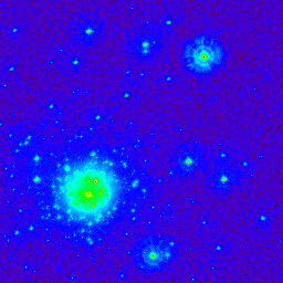
Figure 1: Simulation of an observation of a star cluster through HST before COSTAR correction.

As an example of the results achievable with the previous approach, we consider the reconstruction of a simulated image of HST before COSTAR correction (see Fig. 1), which has already been used to illustrate the performance of space-variant deconvolution methods (see, for instance, Denis et al. 2011; Nagy & O’Leary 1998). The simulated image contains 470 stars on a range of 6 magnitudes with luminosity function and spatial distribution typical of a globular cluster; each of the stars has been convolved with a different PSF. A set of PSF images computed on a $5\times 5$ grid is also included in the data set.

We evaluated the goodness of our reconstruction by comparing the reconstructed image with the so-called ground truth, also available from the ftp, i.e. the true object that is the delta-function source model with no noise. Each source is represented by a pixel having a value equal to the source counts. The stars in the true object are positioned at integer pixel coordinates.

To distinguish between artifacts and stars, we built a threshold map computed by dividing the noise map of the simulated image by the maximum of the local normalized PSF. We obtained the noise map by taking both the photon noise due to the sources and the background and the Gaussian noise due to instrumental effects into account (i.e. RON). We estimated the noise map by means of the XNoise widget procedure included in the StarFinder program (Diolaiti et al. 2000) for astronomical data reduction. The threshold map can therefore be built by portioning the noise map using the same $5\times 5$ PSF grid mentioned above and by dividing each obtained region by the maximum of the associated PSF. This threshold map can be considered as a sort of noise map in the space of the reconstructed image (${\sigma}_{rec}$). It represents, point by point, the value of the reconstructed flux of the sources at the detection limit in the image space. The non-zero pixels in the reconstructed image having a value lower than this threshold map could have been easily generated by noise spikes. They are therefore classified as artifacts. Because of this criterion, all those stars in the reconstructed image that have a value lower than the threshold are non-detectable, even if they have counterparts in the true image. We considered three different thresholds (1, 2 and 3 times the noise map), and we analyzed three main quantities:

• the number of lost stars defined as the number of pixels in the reconstructed image with a value smaller than the threshold and corresponding to pixels of the true image with a value greater than the threshold;

• the number of false detections defined as the number of pixels in the reconstructed image with a value greater than the threshold and corresponding to pixels in the true image with a value equal to zero;

• the error in the reconstructed flux, expressed in magnitudes, evaluated comparing the true magnitudes of the input catalogue used to generate the true image with those derived from the counts in the corresponding pixels of the reconstructed image.

We report in Table 1 the percentage of lost objects and false detections computed by considering the three different thresholds indicated above. We computed the percentage of lost stars considering only the pixels of the true image having a value greater than the threshold. In this case, where we performed no detection and there is severe crowding in the GC centre, this method can cause an overestimation of the false detections. In fact, the light spreading on the adjacent pixels due to a small shift in the centroid of the reconstructed object can originate a small group of false detections around the maxima, representing the true star. To avoid this over-estimation, we should compare the relative maxima inside a certain aperture. This would however cause the blending of sources in the GC centre. We computed the percentage of false detections considering all the pixels of the reconstructed image having a value greater than the threshold. It is apparent that by fixing a reasonable threshold level established by the noise statistic of the image, the number of artifacts that could be confused for stellar sources is quite restrained.

Table 1: Detectability of the sources in the reconstructed image. The total number of sources in the true image is 470.

Threshold	Lost	False
level	stars	detections
1${\sigma}_{rec}$	2.5%	33.4%
2${\sigma}_{rec}$	9.1%	2.6%
3${\sigma}_{rec}$	20.6%	$<1\%$

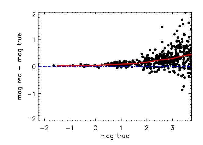
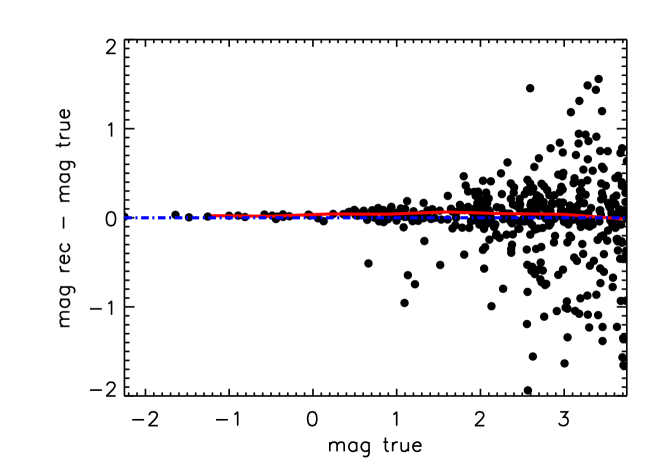
Figure 2: Comparison of the true and reconstructed magnitudes. Upper panel: computed in correspondence of the true stars coordinate pixels. Lower panel: aperture photometry performed in a small region around the source coordinates. The red solid lines show the median error (bin amplitude = 0.5 mag).

The photometric error, due to the error in the source flux reconstruction, is illustrated in the upper panel of Fig. 2. The error is computed comparing the counts of the true image and of the reconstructed image only in the input stars pixel coordinates. The counts that, for some reason, in the reconstructed image fall in the adjacent pixels, get lost. Because of this, the distribution of the magnitude differences shows an evident positively biased asymmetrical trend more prominent in the fainter region of the plot. This trend simply means that the reconstructed flux of the faint sources is spread on a small region of pixels rather than only one, consequently leading to a small source location error (astrometric error). To compute more precisely the reconstructed flux, and so the photometric error, it is necessary to estimate it as the sum of the detected photons within an aperture of pre-fixed radius. This procedure has the drawback of not being independent from the sources crowding, which is rather severe in the cluster core. The crowding causes the attribution of photons coming from stars closer than the aperture radius to the wrong source. Close stars are not clearly distinguishable and the signal belonging to many stars can be attributed to the brighter one, leading to a negatively biased asymmetrical distribution of the errors. This effect is called blending effect. To reduce the blending effect, we adopted apertures with different sizes, depending on the distance from the GC core, and hence, on the crowding. We used apertures from 7 down to 3 pixels in diameter in the external part of the GC, while we only considered a one-pixel aperture in the cluster core. The median value of the photometric error depicted in the bottom panel of Fig. 2 (red line) is now close to zero along the entire magnitude range.

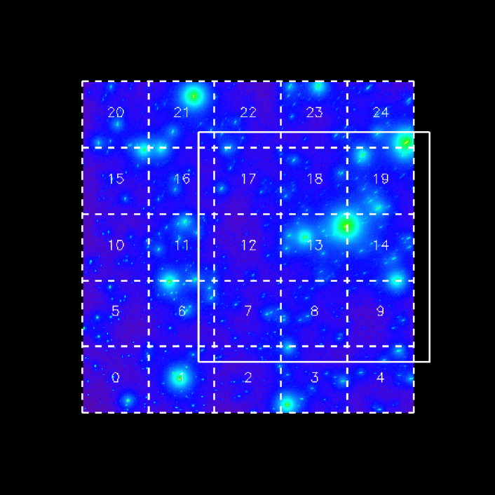
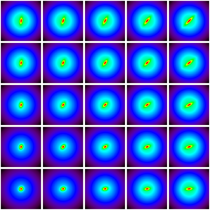
Figure 3: Top panel: the sectioning of the input image (J band) domain into 5$\times$5 overlapping regions; the domain nb 13 is overlaid to show the overlap of the domains. Bottom panel: the 5$\times$5 grid of the PSF, computed from the model described in Appendix B.

3 Image simulation

As in the previous case, images obtained with SCAO systems are characterized by structured PSF, with sharp core and extended halo, and by even more significant variations across the FoV. Up to now, none of the available codes for astronomical data reduction has been specifically designed to account for these PSF characteristics, which are typical of AO systems. The StarFinder code (Diolaiti et al. 2000) was one of the first full attempts to solve the problem of obtaining accurate photometry and astrometry from narrow field AO images with highly structured, but spatially constant, PSF. An effort in this direction has been reported in Schreiber et al. (2012), proposing an upgrade of the StarFinder code to provide it with a set of tools to handle spatially variable PSFs. In the literature, other authors propose the space-variant deconvolution as a necessary tool for the exploitation of AO corrected images (i.e. Fusco et al. 2003; Lauer 2002). In this panorama, AO images offer an interesting test bench for the proposed deconvolution method.

We therefore simulated the observations of an external region of a Galactic globular cluster (GC) in the $J$ band (central wavelength = 1.27 $\mu$m) and in the $K_{s}$ band (central wavelength = 2.12 $\mu$m) with an 8 m class telescope equipped with a SCAO system. The images contain $\sim$ 2800 sources on a range of about 10 magnitudes. The crowding ($\sim$ 6 stars per $arcsec^{2}$) of this field would be severe in seeing limited conditions, while it becomes moderate when using an AO system that shrinks part of the star light in a narrow diffraction limited core. However, the presence of the residual extended halo, which has a size comparable with the seeing, contributes to polluting the field image, enlarging the photometric error and making this case interesting to analyze. More details on the GC relevant parameters and on the characteristics of the image simulation are reported in Appendix A.

The adopted PSF has been modelled to reproduce the main features of a typical SCAO residual PSF and its variation across the FoV. We considered a simple pure analytical model given by the combination of two 2D Moffat components: one representing the sharp diffraction limited core and the other the residual extended seeing halo. The adopted PSF model is described in detail in Appendix B. An example of a simulated frame obtained by this PSF model is depicted in the top panel of Fig. 3. The GS is situated just outside the FoV (bottom left corner). This choice maximizes the PSF variation across a moderate FoV. The Strehl ratio (SR) in both bands rapidly decreases across the FoV, ranging between $0.15$ and almost zero in the $J$ band and between $0.51$ and $0.18$ in the $K_{s}$ band. The maximum SR value corresponds to the GS position, while the minimum value occurs at the opposite image corner. This SR variation indicates a relatively small isoplanatic patch size compared to the FoV: $\theta_{0}\sim 30\arcsec$ in $K_{s}$ band and $\theta_{0}\sim 15\arcsec$ in $J$ band.

4 Data reduction

4.1 Image deconvolution

Starting from the model described in Appendix B, we computed seven different sets of PSFs, namely 3$\times$3, 5$\times$5, 7$\times$7, 9$\times$9, 11$\times$11, 13$\times$13, and 15$\times$15. Each PSF has a fixed size of 512$\times$512 pixels , is positioned on a regular grid across the FoV of the image, and is centred on the centre of each corresponding sub-domain.

In Fig. 3 we show both the input image (top panel) and the grid of the PSFs (bottom panel) for the 5 $\times$ 5 case. As mentioned in Sect. 2.1, the partial overlap of the domains has to be considered. In our simulations we adopt the 95% of the EE of the PSF. In the case of $J$ band, this corresponds to 510 pixels that is always the largest number with respect to all the differences $n_{p}-n$. In the other case ($K_{S}$ band), the extent of the PSF is 170 pixels, which is smaller or equal to the differences $n_{p}-n$. In Fig. 3 (top panel) a sub-domain is put in evidence to show this overlap in the case of J band.

We deconvolved the simulated images using “Patch” which, besides the input image, the number of sub-domains and the corresponding set of PSFs requires the background array (we assumed a constant background), RON and GAIN values (we assumed 20 e^-/pixel and unitary gain, see Table 7). We selected SGP pushed to convergence (iterations are stopped when the objective function described in Eq. 4 is approximately constant, according to a given tolerance, for instance 10^-9). Finally we set a maximum number of 5000 iterations to avoid a possible loop of the algorithm.

In Fig. 4 we show two sub-domains of the 5$\times$5 case before (left panels) and after (right panels) deconvolution. The sources in the reconstructed images look like delta-functions on a black background. The crowding effect due to the PSF extended halos has been largely reduced. Some of the reconstructed sources in the sub-domains more affected by the elongated PSF shape (and so far from the GS), show up a residual elongated pattern, especially close to the sub-domain edges. This is due to the mismatch between the local PSF (defined by an analytical continuous model that depends on the distance from the GS) and the PSF adopted for the sub-domain deconvolution (defined at the centre of the sub-domain). Artifacts, such as dotting, striping or ringing, are more concentrated along the sub-domains edges and around the brightest reconstructed sources. We recall that artifacts can be caused by different factors, like noise spikes or imperfect knowledge of the PSF. As a term of comparison, we also performed all the analysis by deconvolving the images with only one PSF (corresponding to the PSF at the centre of the images). We refer to this result as the 1$\times$1 case. It represents our ‘reference case’, where the proposed method of dividing the image in sub-domains and deconvolving each sub-domain with a local PSF is not applied. A crucial improvement of all the tested quantities is expected.

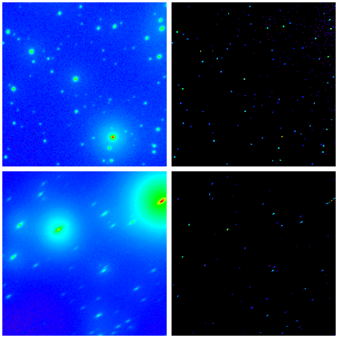
Figure 4: Two sub-domains of the 5$\times$5 case before (left panels) and after (right panels) deconvolution. Referring to Fig. 3 for the sub-domains numeration, sub-domains number 0 and number 13 are represented in the top and bottom panels, respectively.

4.2 Stellar photometry

Aperture photometry can be easily performed on the reconstructed images using apertures of few pixels. Unlike the procedure described in Sect. 2.3, where no detection has been performed in the reconstructed image, we assumed, as in the case of real data, that the positions of the stars in the field are not known. Because of the absence of background (the median value in the reconstructed images is equal to zero) and the delta-function shape of the reconstructed sources, the standard software packages commonly used to perform aperture photometry on astronomical images might be inappropriate in this case. We therefore implemented an on-purpose package of IDL routines, which performs the source finding and the aperture photometry on the reconstructed image, returning a catalogue of fluxes and source coordinates. The objects are identified as relative maxima above a given threshold. The definition of the detection threshold in the space of the reconstructed image ($\sigma_{rec}$) is done as described in Sect. 2.3. We explored the amount of detected and lost objects with different confidence levels (1, 2 and 3$\sigma_{rec}$). We set the aperture diameters differently for each case, being the residual elongation of the sources dependent on the degree of discretization of the PSF. Also the number of generated artifacts around reconstructed sources is related to the local PSF estimation goodness, and hence, with the PSF discretization. Enlarging the aperture diameter allows us to include and recover the counts in the artifacts close to the reconstructed sources. The aperture diameters we adopted decrease from 13 pixels for the widest PSF grid step (3$\times$3 case) to 5 pixels for the finest grid steps (from 9$\times$9 to 15$\times$15 cases). The flux of each source is computed by simply integrating the signal falling into the aperture centred in the source. The star positions have been computed as the centroid on a smaller aperture ($3\times 3$ for all the considered cases) to avoid bias due to the presence of artifacts within the aperture.

5 Results

5.1 Reconstructed image analysis

The reconstructed images are analyzed in terms of percentage of lost objects and number of artifacts.

To quantify the number of non-reconstructed objects, we performed aperture photometry in a very small region (3 pixels diameter) around the input source coordinates. If there are no photons within a given aperture centred in the coordinates of an object listed in the input catalogue (the one used to simulate the image), that object is classified as ‘lost’, and so, not detectable. Table 2 collects the percentages of ‘disappeared’ objects in the reconstructed image with respect to the total number of simulated stars. It is apparent that the number of detected objects becomes closer to the true number of objects by increasing the number of sub-domains, i.e. by reducing the difference between the actual PSF and the one used for the deconvolution of a certain sub-domain. It is interesting to note that if one consider more than 9$\times$9 sub-domains, the quality of the reconstructions does not improve.

This is not a general result, but it depends on the adopted PSF and on its variation model across the FoV. Our model is characterized by a strongly varying core component, and also by a constant halo that contains a high percentage of the star signal, especially in the $J$ band where the SR is lower. The PSF variation, however, is higher in the $K_{s}$ band (see Figs. 8 and 9). This choice allows us to test the boundary effects correction (thanks to the large, but constant halo), to verify the improvement of the image quality when approaching the actual PSF (thanks to the narrow and highly variable core), and to test the robustness of the algorithm to the PSF variation. It is also apparent that the $K_{s}$ band reconstructed image contains a lower percentage of lost objects, probably because of the higher signal-to-noise ratio (SNR), direct consequence of the higher SR.

Table 2: Percentage of lost objects in the image reconstruction process in the $J$ and $K_{s}$ images.

Number of	Lost objects
sub-domains	$J$ band	$K_{s}$ band
$\bf{1\times 1}$	40%	7%
$3\times 3$	23%	3.5%
$5\times 5$	17%	3%
$7\times 7$	16%	3%
$9\times 9$	13%	2.5%
$11\times 11$	13%	2.5%
$13\times 13$	12%	2.5%
$15\times 15$	12%	2.5%

The overall performance seems to take advantage of a better PSF sampling across the FoV. This is also true in terms of photometric accuracy. The number of artifacts that pollute the reconstructed image also decreases when the number of sub-domains increases. This is an expected result in terms of PSF mismatch, but not so obvious in terms of possible unwanted boundary effects that can rise when one splits the image into a large number of sub-images.

To quantify the number of generated artifacts, a source detection has to be performed. The total number of detected objects is given by the sum of the real objects and the artifacts. Since both the reconstructed objects and the artifacts have a delta-function shape, we need to define a method to distinguish between them. As already mentioned, the real objects are identified as relative maxima above a given threshold. As a consequence, all those ‘objects’ that have the maximum lower than the considered threshold are classified as ‘artifacts’. Thanks to this selection, we are able to recognize the majority of the spurious objects, but a residual number of artifacts remains hidden in the output catalogue, namely those artifacts that are above the threshold and have no candidate counterparts within 1 pixel distance in the input catalogue.

Table 3 summarizes the percentages of false detections (or residual artifacts) with respect to the total number of detected stars in the two considered filters and for two different threshold values. It is encouraging to observe that the percentage of artifacts becomes very low for both bands ($\sim$2% and $<$1% in the $J$ and $K_{s}$ bands, respectively) when a 3$\sigma_{rec}$ threshold is adopted. This means that the majority of the spurious objects are relatively faint with respect to the real objects. When more than one image in the same filter is available, a match between different catalogues can filter out some of the remaining spurious objects, especially in low crowding conditions where the probability of ambiguous cases is low. Another interesting result is that the increasing sectioning of the image does not generate an enhancement of spurious sources. In the 15$\times$15 case, the sub-domain size is 69 pixels wide and the adopted PSF (512$\times$512 pixels) has a Moffat halo radius of 20 pixels in the $J$ band (18 pixels in $K_{s}$) comparable to the sub-domain size.

Table 3: Percentage of false detected objects in the reconstructed $J$ and $K_{s}$ images. The percentage is computed with respect to the number of detected stars.

Number of	False detections
sub-domains	$J$ band	$K_{s}$ band
	$1\sigma_{rec}$ / $3\sigma_{rec}$	$1\sigma_{rec}$ / $3\sigma_{rec}$
$\bf{1\times 1}$	60 / 35 %	26 / 13 %
$3\times 3$	52 / 19 %	16 / 3 %
$5\times 5$	35 / 8 %	12 / 1.6 %
$7\times 7$	34 / 7 %	11 / 0.8 %
$9\times 9$	30 / 4 %	11 / 0.7 %
$11\times 11$	28 / 3 %	10 / 0.5 %
$13\times 13$	28 / 2 %	10 / 0.4 %
$15\times 15$	26 / 2 %	9 / 0.4 %

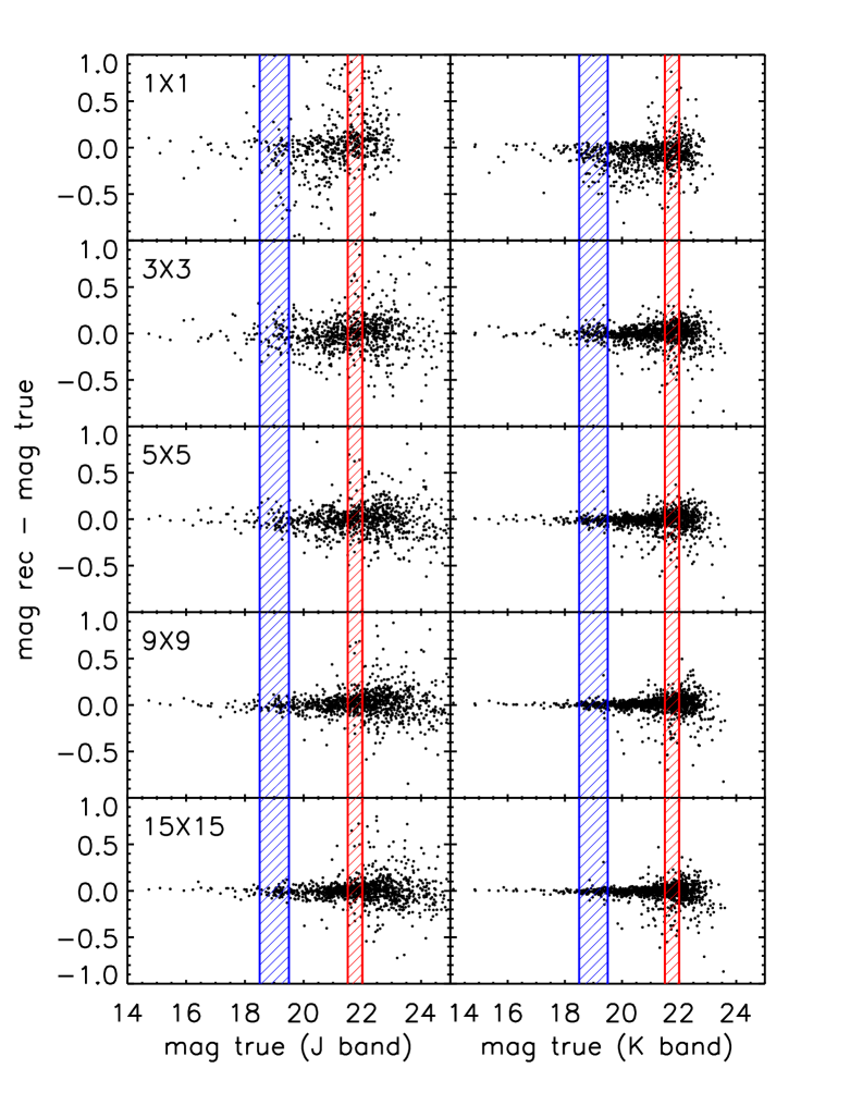
Figure 5: Comparison of the input and measured magnitudes of the detected stars (photometric error) in the $J$ (left column) and $K_{s}$ (right column) bands for some of the analyzed cases. The detection threshold is set to 3$\sigma_{rec}$. From the top: $1\times 1$ (reference case), $3\times 3$, $5\times 5$, $9\times 9$, and $15\times 15$ sub-domains. The blue and red vertical stripes highlight two different bins of magnitudes with amplitude 1 mag (blue stripes) and 0.5 mag (red stripes). The photometric errors relative to the points falling in these stripes are reported in Table 4.

5.2 Photometric accuracy

The photometric accuracy is evaluated for each band and for each case by comparing the true magnitude of the detected stars with that measured from the reconstructed image. Fig. 5 shows a clear improvement in the reconstruction of the source fluxes if the number of sub-domains is increased so that the similarity between the actual PSF and the sub-domain central PSF is increased. This improvement seems to be crucial when one passes from the 3$\times$3 case to the 9$\times$9 case, where the gain starts to decrease considerably for both of the considered bands. The distribution of the magnitude differences looks nicely symmetrical for most of the considered magnitude intervals, and this means that the flux is preserved. As previously discussed, a flux loss would lead to a positively biased distribution. The reference case appears poorly populated as a consequence of the great number of lost objects. We computed the photometric error, defined as the root mean square (r.m.s.) of the differences between the true and the estimated magnitude of the detected stars, in two different bins, one brighter and one fainter, and reported in Table 4. The two considered bins are highlighted in Fig. 5 with the coloured vertical stripes. We chose a wider bin (1 magnitude) to compute the photometric error relative to the brighter sources so that at least 50 sources would fall in the bin for each considered case. In the same two bins, we computed the astrometric error (see Table 5), defined as the r.m.s. of the differences between input and recovered x-coordinate of the stars in a certain magnitude bin. Excluding the $1\times 1$ case, which is reported as a term of comparison, there is no evidence of a strong dependence of the astrometric error on the number of sub-domains. To test for possible drawbacks due to the image sectioning and to our sub-domains approach, we also made the same analysis on a reconstructed image obtained by dividing the image in 15$\times$15 sub-domains and by deconvolving each sub-domain with the same PSF. For this purpose, we used the 1$\times$1 PSF, replicated one time for each sub-domain. The obtained photometric and astrometric errors are in a good agreement with the 1$\times$1 case for both bands, as expected.

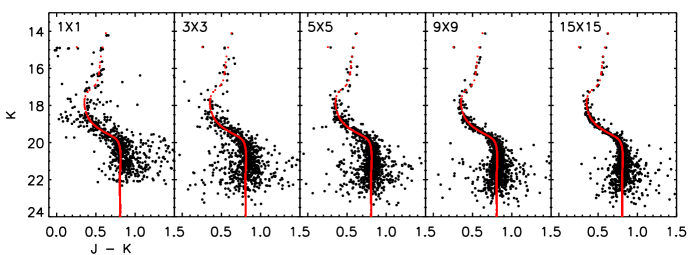
Figure 6: Output ($K$, $J-K$) CMDs for the four image division in sub-domains cases depicted in Fig. 5. The input CMD is over-plotted in red. The detection threshold is set to 3$\sigma_{rec}$ for all cases.

Table 4: Photometric error in the $J$ (second and third columns) and $K_{s}$ (forth and fifth columns) bands computed considering two different bins (called ‘bin 1’ and ‘bin 2’ in the Table). The bins, highlighted in Fig. 5 in blue and red, are defined as follows: bin 1: 18.5 ¡ mag true ¡ 19.5 with amplitude = 1 mag (blue strip); bin 2: 21.5 ¡ mag true ¡ 22 with amplitude = 0.5 mag (red strip).

Number of	Photometric accuracy
sub-domains	$J$ band		$K_{s}$ band
	bin 1	bin 2	bin1	bin 2
$\bf{1\times 1}$	0.17	0.23	0.17	0.19
$3\times 3$	0.14	0.17	0.06	0.10
$5\times 5$	0.09	0.13	0.04	0.08
$7\times 7$	0.06	0.11	0.04	0.08
$9\times 9$	0.05	0.10	0.03	0.07
$11\times 11$	0.05	0.09	0.03	0.06
$13\times 13$	0.05	0.08	0.02	0.06
$15\times 15$	0.04	0.07	0.02	0.06

Table 5: Astrometric error in the $J$ (second and third columns) and $K_{s}$ (forth and fifth columns) bands computed by considering two different bins, as in Table 4. The numbers are given in pixels.

Number of	Astrometric accuracy
sub-domains	$J$ band		$K_{s}$ band
	bin 1	bin 2	bin1	bin 2
$\bf{1\times 1}$	0.27	0.28	0.07	0.15
$3\times 3$	0.05	0.14	0.02	0.12
$5\times 5$	0.05	0.13	0.01	0.11
$7\times 7$	0.05	0.12	0.01	0.11
$9\times 9$	0.03	0.10	0.01	0.10
$11\times 11$	0.03	0.11	0.01	0.10
$13\times 13$	0.03	0.10	0.01	0.10
$15\times 15$	0.02	0.12	0.01	0.10

To better evaluate the quality of the photometry, we combined the output catalogues in the $J$ and $K_{s}$ filters for each case. Fig. 6 shows a selection of the obtained ($K$, $J-K$) colour-magnitude diagrams (CMDs) that refer to the same cases shown in Fig. 5. The input CMD (see Fig. 7) is over-plotted in red. The improvement of the photometric accuracy with increasing number of sub-domains is well represented by the gradual narrowing of all the cluster sequences in the CMD, going from the left to the right of the Figure. A slight quality improvement is also noteworthy between the last two depicted cases (9$\times$9 and 15$\times$15), mostly visible in the bright part of the CMD. This behaviour is confirmed by the photometric errors listed in Table 4, where the values relative to the brighter bins decrease faster with respect to the sources in the fainter bins. The bright sources are reconstructed better than the faint sources. The effect on the CMD depth is also apparent. The depth extends to fainter magnitudes, as a consequence of the decreasing number of lost objects, and therefore, of the increasing number of detected objects (see Table 5). The detection threshold for all the depicted CMDs is set to 1$\sigma_{rec}$. To appreciate the improvement of the overall quality of the CMDs, it is interesting to focus on some features of particular interest in scientific applications, like the Turn Off and the MS knee. The latter, in particular, is a powerful age diagnostic which has become accessible to observation only with the advent of modern AO systems (Bono et al. 2010). The CMD obtained by deconvolving the image with 15$\times$15 PSFs looks very narrow in correspondence of these two features, leading to a more precise fit of the observed isochrone.

6 Conclusions

We propose a sectioning method for reconstructing images corrupted by a space-variant PSF. First of all, the input image is sectioned in partially overlapping sub-domains, the dimensions of which depend on the number, the extent, and the size of the PSFs. Then, each sub-domain (in which we assume that the PSF is space-invariant) is deconvolved with a suitable method with boundary effects correction.

The effectiveness of the proposed method is proved by using two simulated images of stellar fields. The first image (Sect. 2.3) is an image of HST before COSTAR correction, well known in literature. We provide a deep analysis of the results we obtained, giving statistics and photometric error. The second test is the central part of this paper and is a simulation of a globular cluster in the $J$ and $K_{S}$ bands, characterized by a highly structured and variable PSF across the FoV (typical in AO). We simulated the images by employing the continuous model, while we used several discrete grids of PSFs (from 1$\times$1 to 15$\times$15) in the data reduction process. In this sense, we also prove that the method is robust with respect to small variations of the PSF.

In Sect.5, we describe a method for distinguishing artifacts from reconstructed stars, since both have a delta-function shape. The number of artifacts can be controlled by a suitable threshold and, as shown in Table 3, the number of false detections is very small ($\sim$2% and $<$1% in the $J$ and $K_{s}$ bands, respectively) if 3$\sigma_{rec}$ is chosen. Moreover, the number of artifacts and of lost objects decrease when the number of sub-domains increases, i.e. when the difference between the true PSF and the PSF used for deconvolving the sub-domain becomes smaller. We also report good photometric and astrometric results, again with increasing accuracy when the number of sub-domains increases. While there is no evidence of a dependence of the astrometric error on the number of sub-domains, the improvement in the reconstruction of the sources fluxes is crucial starting from the 9$\times$9 case. Moreover, the CMD (obtained by the combination of the results in the two bands) is gradually narrowing and, especially in the 15$\times$15 case, the Turn Off and the MS knee are restored with excellent precision. All the relevant parameters used for the study of the reconstructed image quality (lost objects, artifacts and sources reconstruction) seem to agree on the optimal number of sub-domains to consider. This result, in terms of absolute number of sub-domains, depends mainly on the PSF variation amount across the FoV. The adopted PSF is highly variable across the FoV. A softer PSF variation would lead to performance convergence with a smaller number of sub-domains.

A couple of remarks concludes our paper. The first concerns the deconvolution methods performed in each section. In the Software Patch both RL and SGP algorithms are implemented. In our numerical tests we used SGP, which provides a speed up with respect to RL ranging from 10 to 20 and produces reconstructions with the same, sometimes better, accuracy. Since we considered point-like sources, we pushed the algorithm to convergence with a highly demanding stopping criterion and this demands time. For example the $J$-band 5$\times$5 case requires about 5.8 hours (a mean of about 14 minutes per sub-domain), using a personal computer with an INTEL Core i7-3770 CPU at 3.40GHz and 8 GB of RAM. Even if efficiency is not an issue we consider here, we indicate a few directions for reducing the computational time. First, the processing time can be certainly reduced by choosing a weaker stopping criterion. For example, in the mentioned case, by enlarging the tolerance from $10^{-9}$ to $10^{-5}$, the total processing time is reduced to 53 minutes without changing the quality of the reconstructed image too much: the number of detected objects slightly decreases, while the photometric error increases about 2%. Second, the sectioning method is quite naturally implementable on a multi-processor computer. Moreover, both RL and SGP implementation on GPU has already been considered (Prato et al. 2012), showing that a speed-up of at least 10 is achievable with respect to the serial implementation. Therefore in the case of multi-processors and multi-GPUs a very significant speedup can be achieved, of the order of 100 with 10 GPUs.

The second remark is about PSF extraction and modelling. When handling real astronomical data, the local PSF is generally unknown. Two different approaches have been developed in recent years: the PSF extraction and modelling from the data themselves (Schreiber et al. 2012, 2013), and the PSF reconstruction technique (Veran et al. 1997). The first method involves only post-processing data operations, but it needs suitable stars well distributed across the FoV to model the PSF; the second one could imply the growth of the AO system complexity (especially when MCAO is involved), but it is independent of the observed field. Both methods are interesting when coupled with our deconvolution method, offering a robust and promising tool to reduce astronomical data characterized by a variable PSF. The application of our method to real data using an estimated PSF is still under investigation and will be published in a future paper.

The IDL code of the method described in this paper is available on the software section of the website http://www.airyproject.eu.

Appendix A Globular cluster image parameters

The simulated GC is located at a distance of 10 kpc and is 12 giga-years old. We selected a region located at the half-mass radius of the cluster, at a distance of $128\arcsec=6.2$ pc from the cluster centre. All the relevant parameters of the synthetic cluster are listed in Table 6. The magnitudes and colours of the synthetic member stars have been drawn from theoretical models, the physical positions from N-body realizations of an equilibrium King (1966) model. The observations were ‘acquired’ with a fictitious, but realistic, 8.2 meters telescope equipped with a SCAO system + science camera + detector whose main characteristics are reported in Table 7. These characteristics are very similar to the PISCES Infrared Imager with the Large Binocular Telescope Adaptive Optics System (Guerra et al. 2013). A set of $J$ (central wavelength = 1.27 $\mu$m) and $K_{s}$ (central wavelength = 2.12 $\mu$m) band images have been simulated. The fraction of stars falling in the frames ($\sim 2800$ stars having $J\la 25$ mag and $K_{s}\la 24.2$ mag) is highlighted in red in Fig. 7. To detect stars up to at least two magnitudes below the main-sequence (MS) knee, we fixed the total exposure time for each image to 1 hour for both bands. Therefore we computed the time for the individual exposures to avoid the saturation of any star. The $J$ band image is the result of the sum of 180 exposures of 20 seconds each, while the $K_{s}$ band image is the result of the sum of 240 exposures of 15 seconds each.

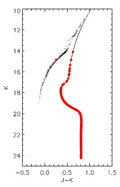
Figure 7: The near-IR CMD of the GC stellar population. The total mass of the stars, formed 12 Gyr ago, is $5.4\times 10^{5}$ M_☉. The red dots highlight the sub-sample of the entire population that fall in the FoV considered in our simulation.

Table 6: Parameters of the synthetic cluster. The assumed distribution is based on the King (1996) equilibrium model. HB and IMF mean horizontal branch and initial mass function.

C (W0)	1.9 (8.0)
Core radius	0.75 pc
Tidal radius	60 pc
N(stars)	$2\times 10^{6}$
Stellar theoretical models	Dotter et al. (2008)
Total Mass (stars)	$5.4\times 10^{5}$ M☉
Age of Stars	12 Gyr
$[Fe/H]/[\alpha/Fe]$	$-0.40/0.00$
IMF	$N(m)\propto m^{-1.35}$
HB: mean mass / $\sigma_{mass}$	$0.60/0.04$ M☉
Binary Fraction	0.0%
Assumed distance	10.0 Kpc
Assumed reddening	E(B-V)=0.0

Table 7: Telescope + Camera + Detector parameters adopted for the simulation. We assumed the average values of the sky surface brightness at Mount Graham (Pedani 2014).

Collecting area	50 m2
FoV	$21.5\arcsec\times 21.5\arcsec$
Detector dimension	$1024\times 1024$ px
Pixel scale	$0.021\arcsec$
Gain	1 $e^{-}$/ADU
Read-out noise	20 $e^{-}$
QE	60% in J band
Saturation Level	$\ga$ 40000 ADU
Dark current	$0.1$ $e^{-}$/sec
Sky background mag	15.82, 13.42
($J$ and $K_{s}$ bands)

Appendix B PSF model

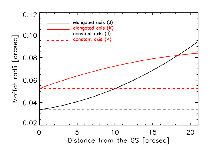
Figure 8: Variation of the radii of the Moffat Core components of the PSFs in $J$ (black curves) and $K_{s}$ (red curves) bands across the FoV with respect to the GS distance in arcseconds. The continuous lines refer to the elongated radii of the Moffats. The dashed lines refer to the non-elongated radii of the Moffats. The non-elongated radii have been considered constant in this simplified model.

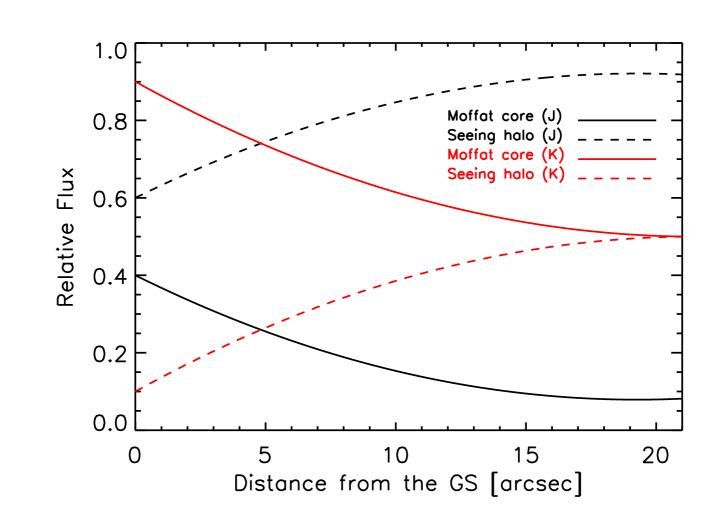
Figure 9: Variation with respect to the GS distance of the relative flux contained in each of the two PSF components: core (continuous lines) + halo (dashed lines).

At a first approximation, the AO PSFs can be approximated by the combination of different analytical components, such as Moffat, Lorentzian, or Gaussian 2D functions, their parameters varying with respect to the position in the FoV (Schreiber et al. 2011). To simulate images with a continuous space-variant PSF, we considered a simple pure analytical model given by the combination of two 2D Moffat components:

• Diffraction limited core: Moffat with a radial variation with respect to the guide star (GS) direction. The rotation angle reproduces the typical SCAO elongation pattern pointing towards the GS. The variation of the two Moffat half-light radii with respect to the distance from the GS is plotted in Fig. 8. As depicted in Fig. 8, the half-light radius pointing in the direction of the GS (i.e. along the elongated axis) is variable across the FoV and its variation is described by a polynomial function of the distance of the PSF location in the image from the reference position. The half-light radius pointing orthogonally towards this direction has been considered constant and close to the diffraction limit.

• Seeing halo: round Moffat (no elongation). The radius of this component (20 pixels in $J$ and 18 pixels in $K_{s}$) has been set to reproduce a seeing disk of $\sim 0.6\arcsec$ in $J$ band. The only variable parameter in the FoV is the relative flux $F_{Halo}=1-F_{Core}$, where $F_{Core}$ is the relative flux contained in the core component. The halo component contains the signal due to the residual non-corrected atmospheric aberrations and, therefore, its relative flux grows with the GS distance following a second order polynomial trend. Fig. 9 reports the variation of the flux distribution among the two PSF components (core and halo) in the two considered bands ($J$ and $K_{s}$) with respect to the GS distance.