How to calculate quantum quench distributions with a weighted Wang-Landau Monte Carlo

Abstract

We present here an extension of the Wang-Landau Monte Carlo method which allows us to get very accurate estimates of the full probability distributions of several observables after a quantum quench for large systems, whenever the relevant matrix elements are calculable, but the full exponential complexity of the Hilbert space would make an exhaustive enumeration impossible beyond very limited sizes. We apply this method to quenches of free-fermion models with disorder, further corroborating the fact that a Generalized Gibbs Ensemble fails to capture the long-time average of many-body operators when disorder is present.

1 Introduction

A sudden quench of the Hamiltonian parameters is perhaps the simplest form of out-of-equilibrium dynamics that a closed quantum system can experience. Experiments with “virtually isolated” cold atomic species in optical lattices [1, 2] have transformed this seemingly theoretical dream into a rich and lively stage. Several fundamental issues of theoretical quantum statistical physics, like the onset of thermalization which is generally expected to occur for a closed quantum system after a sudden quench [3, 4, 5], or the “breakdown of thermalization” [6, 7] expected when the system is integrable or nearly integrable, are now of experimental relevance [8]. We refer the reader to a recent review [9] for an extensive introduction to such non-equilibrium quantum dynamics issues.

The issue we want to tackle in this paper is the following. Suppose you perform a quantum quench of the Hamiltonian parameters, abruptly changing, at $t=0$, from $\hat{H}_{0}\to\hat{H}$. If $|\Psi_{0}\rangle$ denotes the initial quantum state at $t=0$, and $|\alpha\rangle$ the eigenstates of $\hat{H}$ with energy $E_{\alpha}$, the ensuing quantum dynamics would lead to averages for any given operator $\hat{A}$ given by:

$$A(t)\equiv\langle\Psi_{0}|e^{i\hat{H}t}\hat{A}e^{-i\hat{H}t}|\Psi_{0}\rangle=\sum_{\alpha}|c_{\alpha}|^{2}A_{\alpha\alpha}+\sum_{\alpha^{\prime}\neq\alpha}e^{i(E_{\alpha^{\prime}}-E_{\alpha})t}c_{\alpha^{\prime}}^{*}A_{\alpha^{\prime}\alpha}c_{\alpha}\;,$$ (1)

where $c_{\alpha}\equiv\langle\alpha|\Psi_{0}\rangle$ and $A_{\alpha^{\prime}\alpha}\equiv\langle\alpha^{\prime}|\hat{A}|\alpha\rangle$. The first (time-independent) term in the previous expression dominates the long-time average of $A(t)$, and is usually known as diagonal average [5]

$$\langle\hat{A}\rangle_{\mathrm{\scriptscriptstyle D}}\equiv\sum_{\alpha}\left|c_{\alpha}\right|^{2}A_{\alpha\alpha}\;.$$ (2)

To calculate it, in principle, we should take the sum over all the (many-body) eigenstates $|\alpha\rangle$ of $\hat{H}$ — an exponentially large number of states —, calculating for each of them the overlap $c_{\alpha}$ and the associated diagonal matrix element $A_{\alpha\alpha}$. Luckily, $\langle\hat{A}\rangle_{\mathrm{\scriptscriptstyle D}}$ can be calculated for many problems, notably those that can be reduced to quadratic fermionic problems, by circumventing in one way or another exponentially large sums: for instance, through a detour to time-dependent single-particle Green’s function and the use of Wick’s theorem, see e.g.  [10, 11]. But suppose that you want to know more than just the diagonal average $\langle\hat{A}\rangle_{\mathrm{\scriptscriptstyle D}}$, and pretend to have information on the whole distribution of the values of $A_{\alpha\alpha}$ accessed after the quench [12, 13], i.e.,

$$\rho_{\mathrm{\scriptscriptstyle D}}(A)\equiv\sum_{\alpha}\left|c_{\alpha}\right|^{2}\delta(A-A_{\alpha\alpha})\;,$$ (3)

of which $\langle\hat{A}\rangle_{\mathrm{\scriptscriptstyle D}}$ is just the average: $\langle\hat{A}\rangle_{\mathrm{\scriptscriptstyle D}}=\int\!\mathrm{d}A\,\rho_{\mathrm{\scriptscriptstyle D}}(A)\;A$. Here there is, evidently, a problem: knowing the distribution of $A$ requires exploring the full many-body Hilbert space, summing over the eigenstates $|\alpha\rangle$, and this exhaustive enumeration would restrict our calculations to exceedingly small sample sizes, although all information on $c_{\alpha}$ and $A_{\alpha\alpha}$ might in principle be easy to calculate, or in any case accessible, for instance by just solving a one-body problem (hence, for much larger sizes). A similar problem occurs in considering, for instance, the corresponding  generalized Gibbs ensemble (GGE) average [14, 15, 16, 17, 18]

$$\langle\hat{A}\rangle_{\mathrm{\scriptscriptstyle GGE}}\equiv\sum_{\alpha}\frac{\mathrm{e}^{-\sum_{\mu}\lambda_{\mu}I_{\mu}^{\alpha}}}{Z_{\mathrm{\scriptscriptstyle GGE}}}A_{\alpha\alpha}\;,$$ (4)

where $\lambda_{\mu}$ are Lagrange multipliers which constrain the mean value of each of the constants of motion $\hat{I}_{\mu}$ to their $t=0$ value, $\langle\Psi_{0}|\hat{I}_{\mu}|\Psi_{0}\rangle=\Tr\left[\hat{\rho}_{\mathrm{\scriptscriptstyle GGE}}\hat{I}_{\mu}\right]$, $I_{\mu}^{\alpha}\equiv\langle\alpha|\hat{I}_{\mu}|\alpha\rangle$, $Z_{\mathrm{\scriptscriptstyle GGE}}$ is the GGE partition function, and $\hat{\rho}_{\mathrm{\scriptscriptstyle GGE}}\equiv e^{-\sum_{\mu}\lambda_{\mu}\hat{I}_{\mu}}/Z_{\mathrm{\scriptscriptstyle GGE}}$. Once again, for “quadratic problems” this average is rather simply calculated in terms of single-particle quantities, but the corresponding distribution

$$\rho_{\mathrm{\scriptscriptstyle GGE}}(A)\equiv\sum_{\alpha}\frac{\mathrm{e}^{-\sum_{\mu}\lambda_{\mu}I_{\mu}^{\alpha}}}{Z_{\mathrm{\scriptscriptstyle GGE}}}\delta(A-A_{\alpha\alpha})\;,$$ (5)

requires a difficult sum over the Hilbert space.

Concerning the issue of thermalization after a quantum quench, we might indeed expect that, if the system is well described by a GGE ensemble, not only the mean values of $\rho_{\mathrm{\scriptscriptstyle D}}(A)$ and $\rho_{\mathrm{\scriptscriptstyle GGE}}(A)$ are equal, i.e., $\langle\hat{A}\rangle_{\mathrm{\scriptscriptstyle D}}\equiv\int\mathrm{d}A\,\rho_{\mathrm{\scriptscriptstyle D}}(A)A=\langle\hat{A}\rangle_{\mathrm{\scriptscriptstyle GGE}}\equiv\int\mathrm{d}A\,\rho_{\mathrm{\scriptscriptstyle GGE}}(A)A$, but also the two distributions should be closely related; at least this is what a good statistical ensemble should do.

Quite generally, we might formulate the problem as follows: how can we obtain information on weighted distributions (or density of states)

$$\rho_{\mathrm{w}}(A)\equiv\sum_{\alpha}w_{\alpha}\delta(A-A_{\alpha})\;,$$ (6)

with positive weights $w_{\alpha}$, when both $w_{\alpha}$ and $A_{\alpha}$ are “easily calculated”, but the sum over $\alpha$ runs over an exponentially large “configuration space”? As discussed before, examples of this are the diagonal distribution, where $w_{\alpha}=|c_{\alpha}|^{2}$, the GGE distribution, where $w_{\alpha}=\mathrm{e}^{-\sum_{\mu}\lambda_{\mu}I_{\mu}^{\alpha}}/Z_{\mathrm{\scriptscriptstyle GGE}}$, but also the microcanonical distribution, where $w_{\alpha}$ is a window characteristic function for the microcanonical shells, etc. A Monte Carlo algorithm to perform such exponentially large sums in configuration space seems unavoidable. We stress that this is so even if one is considering quenches in free-fermion models, where the relevant many-particle states $|\alpha\rangle$ and matrix elements are easy to write down and calculate. The alternative of using exact diagonalization methods would put a strong limit on the size of the problem which can be studied.

In this paper we introduce a Monte Carlo method — obtained by a rather natural extension of the Wang-Landau algorithm (WLA) [19, 20, 21] — which will allow us to compute weighted distributions of the form of Eq. (6). The Wang-Landau algorithm, proposed in 2001 by F. Wang and D.P. Landau, is a Monte Carlo method designed to compute the density of states of a classical statistical mechanics problem. The algorithm performs a non-Markovian random walk to build the density of states by overcoming the prohibitively long time scales typically encountered near phase transitions or at low temperatures. Besides the classical Ising and Potts models studied in the original papers [19, 20, 21], the method has been applied to the solution of numerical integrals [22], folding of proteins [23] and many other problems.

Here is the plan of the paper. In Sec. 2 we show how the WLA can be extended to compute weighted density of states. In Sec. 3 we show how the weighted-WLA can be used to compute distributions related to quantum quenches with quadratic fermionic models. Finally, Sec. 4 contains a summary and future perspectives.

2 Weighted Wang-Landau algorithm

Let us consider a system with a discrete configuration space, where configurations can be labeled with an index $\alpha$. Given a physical observable $\hat{A}$, we define its weighted (coarse-grained) density of states:

$$\rho_{\mathrm{w}}(A)\equiv\sum_{\alpha}w_{\alpha}\delta_{AA_{\alpha}}\;,$$ (7)

with $w_{\alpha}$ a positive weight. Here $\delta_{AA_{\alpha}}$ is a Kronecker delta, or, if the possible values of $A_{\alpha}$ are too dense to keep them all, a suitable histogram-window-function coarse-graining of the Dirac’s delta. When $w_{\alpha}=1$, we recover the usual density of states $\rho(A)$, and the WLA can be used to estimate it [19, 20, 21]. We will now show that, by properly modifying the WLA, we can compute $\rho_{\mathrm{w}}(A)$ for generic $w_{\alpha}$s.

To understand the gist of the approach, consider a generic positive function $\tilde{\rho}_{\mathrm{w}}(A)$ — which is our best guess for the desired $\rho_{\mathrm{w}}(A)$ —, and set up a Markov chain random walk in which, given a state $\alpha$, a new state $\alpha^{\prime}$ is generated with a trial probability $T(\alpha^{\prime}|\alpha)$, which we will take to be symmetric, $T(\alpha^{\prime}|\alpha)=T(\alpha|\alpha^{\prime})$, and accepted with probability:

$$R(\alpha^{\prime}|\alpha)=\mathrm{Min}\left[1,\frac{w_{\alpha^{\prime}}}{w_{\alpha}}\frac{\tilde{\rho}_{\mathrm{w}}(A_{\alpha})}{\tilde{\rho}_{\mathrm{w}}(A_{\alpha^{\prime}})}\frac{T(\alpha|\alpha^{\prime})}{T(\alpha^{\prime}|\alpha)}\right]\;.$$ (8)

With this standard Metropolis Monte Carlo prescription, we know that, after an initial transient, we will visit the configurations $\alpha$ with an equilibrium distribution $P^{\rm eq}_{\alpha}$ fulfilling the detailed balance condition and given by:

$$P^{\rm eq}_{\alpha}=C\frac{w_{\alpha}}{\tilde{\rho}_{\mathrm{w}}(A_{\alpha})}\;,$$

where $C$ is a normalization constant. As in the WLA [19], while the random walk goes on, we collect a histogram $h(A)$, updating $h(A_{\alpha})\to h(A_{\alpha})+1$ at each visited state $\alpha$. At equilibrium, after $N_{s}$ steps, the “mean” histogram will then be given by:

$$h(A)=N_{s}\sum_{\alpha}P^{\rm eq}_{\alpha}\,\delta_{AA_{\alpha}}=N_{s}C\,\sum_{\alpha}\frac{w_{\alpha}}{\tilde{\rho}_{\mathrm{w}}(A_{\alpha})}\delta_{AA_{\alpha}}=N_{s}C\,\frac{\rho_{\mathrm{w}}(A)}{\tilde{\rho}_{\mathrm{w}}(A)}\;.$$ (9)

Exactly as for the WLA [19], if our guess for $\tilde{\rho}_{\mathrm{w}}(A)$ is a good approximation to $\rho_{\mathrm{w}}(A)$, the histogram $h(A)$ will be “almost flat” (see below). Obviously, during the random walk, together with the histogram $h(A)$ we also update our guessed $\tilde{\rho}_{\mathrm{w}}(A)$. Therefore, closely inspired by the WLA [19], we propose the following algorithm:

1. Fix a modification factor $f>1$, and set $\ln\tilde{\rho}_{\mathrm{w}}(A)=0$ and $h(A)=0$ for all values of $A$;

2. Start the Monte Carlo procedure using Eq. (8) and update at each step the histogram and the weighted density of states with the rules $h(A_{\alpha})\rightarrow h(A_{\alpha})+1$ and $\ln\tilde{\rho}_{\mathrm{w}}(A_{\alpha})\rightarrow\ln\tilde{\rho}_{\mathrm{w}}(A_{\alpha})+\ln f$;

3. Stop the random walk when $h(A)$ is “almost flat” (for instance [19], when $h(A)>0.8\overline{h}$ for all values of $A$, where $\overline{h}$ is the mean histogram value). For the previous observations, at the end of this step $\ln\tilde{\rho}_{\mathrm{w}}(A)$ is a good approximation to $\ln\rho_{\mathrm{w}}(A)$ with a discrepancy of order $\ln f$;

4. Reduce the value of $f\to\sqrt{f}$, reset $h(A)=0$ and restart the procedure from step (1) using the $\tilde{\rho}_{\mathrm{w}}(A)$ just obtained. Stop this loop when $\ln f$ is smaller than the desired discrepancy $\epsilon$.

A similar extension of the WLA has been already been introduced for the particular case in which $w_{\alpha}$ is the Boltzmann distribution, with the aim of computing the free energy profile as a function of a reaction coordinate [24, 25]. In the present paper, we will use this algorithm to compute distributions where the weights are not Boltzmann-like, but rather associated to quantum quenches.

Let us return for a moment to the original WLA. A first trivial observation is that, as it should be, the weighted-WLA with $w_{\alpha}=1/N$ coincides with the WLA. In many situations, when the size of the configuration space is too big and the density of states ranges over too many orders of magnitude, it is convenient, in computing $\rho(A)$, to run many WLA over small domains $\Delta^{(i)}_{A}=[A_{\mathrm{min}}^{(i)},A_{\mathrm{max{\phantom{i}}\!}}^{(i)}]$. But then the update rule of the standard WLA has to be changed to avoid that, during the random walk, $A_{\alpha}$ leaves the domain $\Delta^{(i)}_{A}$. This trick was already used in the first papers by Wang and Landau, when dealing with the largest sizes [19]. To avoid leaks from $\Delta^{(i)}_{A}$, the empirical solution was to reject any proposal to states $\alpha^{\prime}$ with $A_{\alpha^{\prime}}\notin\Delta^{(i)}_{A}$, without any update of $\tilde{\rho}(A)$ and $h(A)$. With this prescription, however, there are “boundary effects”, actually a systematic underestimation of the density of states at the borders of the intervals [26]. Schulz et al. [26] showed phenomenologically that such boundary effects are eliminated by using the rather obvious update rule: given a proposal $\alpha^{\prime}$, if $A_{\alpha^{\prime}}$ is outside the interval we remain in $\alpha$ and we update $h(A)$ and $\ln\tilde{\rho}(A)$ using the state $\alpha$, otherwise we accept $\alpha^{\prime}$ with the usual rule. This update rule is just what is obtained, rigorously, by using our weighted-WLA. Indeed, the density of states in a restricted range $\Delta^{(i)}_{A}$ is proportional to a weighted density of states in which $w_{\alpha}=1$ when $A_{\alpha}\in\Delta^{(i)}_{A}$, and zero otherwise. With these weights, the update rule of our weighted-WLA is exactly the one obtained phenomenologically by Schulz et al. [26].

3 Quantum quenches

In this section we come back to the initial problem of computing the distributions $\rho_{\mathrm{\scriptscriptstyle D}}(A)$ and $\rho_{\mathrm{\scriptscriptstyle GGE}}(A)$ related to quantum quenches. We will show that with the weighted-WLA we can compute these distributions for sizes inaccessible with an exhaustive enumeration.

We concentrate on quantum quenches in two models possessing a free fermionic description. The first model we considered is the fermionic Anderson model with disorder in the local potential:

$$\hat{H}_{\mathrm{A}}\equiv-t\sum_{j=1}^{L}\left(\hat{c}_{j}^{\dagger}\hat{c}_{j+1}+\mathrm{h.c.}\right)+\sum_{j=1}^{L}h_{j}\hat{c}^{\dagger}_{j}\hat{c}_{j}\;,$$ (10)

where $\hat{c}_{j}^{\dagger}$ ($\hat{c}_{j}$) creates (destroys) a fermion at site $j$, $t$ is the nearest-neighbor hopping integral and $h_{j}$ is an uncorrelated on-site random potential uniformly distributed in the range $\left[-W/2,W/2\right]$. We assume periodic boundary conditions. It has been mathematically proven [27] that, for Hamiltonians like $\hat{H}_{\mathrm{A}}$ and in presence of any $W>0$, all the single-particle eigenstates of $\hat{H}_{\mathrm{A}}$ are exponentially localized. The second model we considered still describes spinless fermions hopping on a chain, but now the hopping is long-ranged [28]:

$$\hat{H}_{\mathrm{lrh}}=\sum_{j_{1}j_{2}}t_{j_{1}j_{2}}(\hat{c}_{j_{1}}^{\dagger}\hat{c}_{j_{2}}+\mathrm{h.c.})\;,$$ (11)

where $t_{j_{1}j_{2}}$ is a (real) hopping integral between sites $j_{1}$ and $j_{2}$. We will take the $t_{j_{1}j_{2}}$’s to be random and long-ranged, with a Gaussian distribution of zero mean, $\langle t_{j_{1}j_{2}}\rangle=0$, and variance given by:

$$\langle t_{j_{1}j_{2}}^{2}\rangle=\frac{1}{1+\left(\frac{|j_{1}-j_{2}|}{\beta}\right)^{2\gamma}}\,.$$ (12)

Here $\gamma$ is a real positive parameter setting how fast the hoppings’ variance decays with distance. Notice that, for $j_{1}=j_{2}$, we have $\langle t_{j_{1}j_{2}}^{2}\rangle=1$ for any $\gamma$, hence the model has also on-site Gaussian disorder; by increasing the distance between the two sites $|j_{1}-j_{2}|$, the variance of the hopping integral decreases with a power law. The peculiarity of this long-range-hopping model is that, although being one-dimensional and regardless of the value of $\beta$ (which hereafter is fixed to $1$), it has an Anderson transition from (metallic) extended eigenstates, for $\gamma<1$, to (insulating) power-law localized eigenstates for $\gamma>1$ [28, 29, 30]. Physically, this is due to the fact that, for small $\gamma$, long-range hoppings are capable of overcoming the localization due to disorder. Having access, in the same model, to physical situations in which the final eigenstates are extended ($\gamma<1$) or localized ($\gamma>1$) will clearly show the role that spatial localization plays in disrupting the ability of the GGE to describe the after-quench dynamics. Physically, spatial localization prevents the different “modes” of the system from having an infinite reservoir.

For the considered quenches, we use as initial Hamiltonian $\hat{H}_{0}$ the clean chain with $W=0$ and the same boundary conditions of the final Hamiltonian, i.e., periodic boundary conditions when quenching to $\hat{H}_{\mathrm{A}}$ and open boundary conditions when quenching to $\hat{H}_{\mathrm{lrh}}$. The corresponding initial state $|\Psi_{0}\rangle$ will be the filled Fermi sea, i.e., the ground state of $\hat{H}_{0}$ with $N_{\mathrm{F}}=L/2$, where $N_{\mathrm{F}}$ is the number of fermions. The reason behind this simple choice for $\hat{H}_{0}$ is that the “stationary state” reached does not depend, qualitatively, on the initial Hamiltonian being ordered or not, see Ref. [10]. The final Hamiltonian will be the Anderson model $\hat{H}_{\mathrm{A}}$ with $W=2$, or the long-range hopping chain $\hat{H}_{\mathrm{lrh}}$ with $\gamma=0.5$ or $2$. In all cases the particle number is a constant of motion, therefore $N_{\mathrm{F}}=L/2$ for any time $t>0$. To get a smoother size dependence of the computed quantities, the smaller size realizations are obtained by cutting an equal amount of sites at the two edges of the largest realization.

The two Hamiltonians, being quadratic in the fermion operators, can be diagonalized for any chain of size $L$ in terms of new fermionic operators

$$\hat{d}_{\mu}^{\dagger}=\sum_{j=1}^{L}u_{j\mu}\hat{c}_{j}^{\dagger}\;,$$ (13)

where $u_{j\mu}$ are the wave functions of the eigenmodes of energy $\epsilon_{\mu}$: $\hat{H}_{\mathrm{A}/\mathrm{lrh}}=\sum_{\mu}\epsilon_{\mu}\hat{d}_{\mu}^{\dagger}\hat{d}_{\mu}$. The energies $\epsilon_{\mu}$ and the associated wave functions $u_{j\mu}$ are obtained, for any given disorder realization of a chain of size $L$ by numerically diagonalizing the $L\times L$ one-body hopping matrix.

Given an observable $\hat{A}$, consider the two distributions introduced before:

$$\rho_{\mathrm{\scriptscriptstyle D}}(A) \equiv \sum_{\alpha}|c_{\alpha}|^{2}\delta(A-A_{\alpha\alpha})$$ (14)

$$\rho_{\mathrm{\scriptscriptstyle GGE}}(A) \equiv \sum_{\alpha}\frac{\mathrm{e}^{-\sum_{\mu}\lambda_{\mu}n_{\mu}^{\alpha}}}{Z_{\mathrm{\scriptscriptstyle GGE}}}\delta(A-A_{\alpha\alpha})\;,$$ (15)

where $\delta(x)$ is the Dirac’s delta, $\{|\alpha\rangle\}$ are the many-body eigenstates of $\hat{H}$, $A_{\alpha\beta}\equiv\langle\alpha|\hat{A}|\beta\rangle$, $c_{\alpha}\equiv\langle\alpha|\Psi_{0}\rangle$, and $n_{\mu}^{\alpha}=0,1$ is the occupation of the single-particle eigenstate $\mu$ in the many-body eigenstate $|\alpha\rangle$. These functions give the weighted distributions of $A_{\alpha\alpha}$ in the diagonal and GGE ensembles.

Let us discuss a few technical details on the implementation we made, before discussing the physics emerging from our calculations. Notice that the sum over $\alpha$ is effectively restricted to the canonical Hilbert space ${\mathcal{H}}_{N}$ with a fixed number of particles $N=N_{\mathrm{F}}$ in the diagonal ensemble, since $c_{\alpha}\equiv\langle\alpha|\Psi_{0}\rangle=0$ if $N_{\alpha}\neq N_{\mathrm{F}}$. No such restriction is in principle present in the GGE case, where the sum over $\alpha$ runs over the grand-canonical Hilbert space. By definition, the distributions are such that $\langle\hat{A}\rangle_{\mathrm{\scriptscriptstyle D}}=\int\!A\,\rho_{\mathrm{\scriptscriptstyle D}}(A)\,\mathrm{d}A$ and $\langle\hat{A}\rangle_{\mathrm{\scriptscriptstyle GGE}}=\int\mathrm{d}A\,\rho_{\mathrm{\scriptscriptstyle GGE}}(A)A$, where the integration is over the domain of $A_{\alpha\alpha}$. As customary in any numerical finite-size study, one really needs to consider a coarse-grained version of these distributions, obtained by splitting the domain of $A$ into small intervals $\Delta^{(i)}$ of amplitude $\Delta$. Such a coarse-grained distribution has exactly the form of a weighted density of states, see Eq. (7), with $w_{\alpha}=\left|c_{\alpha}\right|^{2}/\Delta$ in the diagonal case, and $w_{\alpha}=\mathrm{e}^{-\sum_{\mu}\lambda_{\mu}n_{\mu}^{\alpha}}/(\Delta\;Z_{\mathrm{\scriptscriptstyle GGE}})$ in the GGE case. The configuration space $\{|\alpha\rangle\}$ (i.e., the canonical Hilbert space ${\mathcal{H}}_{N}$ for the diagonal distribution and the full Hilbert space for the GGE) over which the two weighted distributions are defined is discrete and grows exponentially with the system size. The weighted-WLA is therefore the appropriate tool for the numerical computation of $\rho_{\mathrm{\scriptscriptstyle D}}(A)$ and $\rho_{\mathrm{\scriptscriptstyle GGE}}(A)$. The eigenstates $|\alpha\rangle$ which appear in the definition of $\rho_{\mathrm{\scriptscriptstyle D}}(A)$ have a fixed number of fermions $N_{\mathrm{F}}$ (the same of the initial state), while in $\rho_{\mathrm{\scriptscriptstyle GGE}}(A)$ the number of particles can change. In the weighted-WLA, for the diagonal ensemble, we use therefore a “particle conserving” proposal scheme: given a state $|\alpha\rangle$, the state $|\alpha^{\prime}\rangle$ is given by moving at random a fermion in one of the unoccupied single-particle eigenstates. In this case, the ratio $w_{\alpha^{\prime}}/w_{\alpha}$ which appears in Eq. (8), is equal to:

$$\frac{w_{\alpha^{\prime}}}{w_{\alpha}}=\frac{\left|c_{\alpha^{\prime}}\right|^{2}}{\left|c_{\alpha}\right|^{2}}\;,$$

where the coefficient $|c_{\alpha}|^{2}$ is the square of the determinant of a $N_{\mathrm{F}}\times N_{\mathrm{F}}$ matrix (see [31, App. D] for the explicit expression of $|c_{\alpha}|^{2}$). For the GGE case, instead, we do not have restrictions on the number of fermions and, given a state $|\alpha\rangle$, we generate a state $|\alpha^{\prime}\rangle$ by changing the occupation of a randomly selected single-particle eigenstate $\mu$. In this case:

$$\frac{w_{\alpha^{\prime}}}{w_{\alpha}}=\mathrm{e}^{\pm\lambda_{\mu}}\;,$$

where the $+$ ($-$) sign appears when the mode $\mu$ is initially occupied (empty). Let us recall that the Lagrange’s multipliers $\lambda_{\mu}$ are obtained by requiring $\langle\Psi_{0}|\hat{d}_{\mu}^{\dagger}\hat{d}_{\mu}|\Psi_{0}\rangle=\langle\hat{d}_{\mu}^{\dagger}\hat{d}_{\mu}\rangle_{\mathrm{\scriptscriptstyle GGE}}$. This condition, written explicitly, reads:

$$\mathrm{e}^{\lambda_{\mu}}=\frac{1}{\sum_{\nu}n_{\nu}^{0}\left|\left[u^{0\dagger}u\right]_{\nu\mu}\right|^{2}}-1\;,$$ (16)

where $u^{0}$ and $u$ are $L\times L$ matrices whose elements $u_{j\nu}^{0}$ and $u_{j\mu}$ are the single-particle wavefunctions of the initial Hamiltonian $\hat{H}_{0}$ and the final one $\hat{H}$, and $n^{0}_{\nu}=0,1$ is the occupation of the $\nu$th eigenstate of $\hat{H}_{0}$ in the initial state. The difference in the computational effort on computing the ratio $w_{\alpha^{\prime}}/w_{\alpha}$ in the two ensembles is evident: in the diagonal case at each step we have to compute the determinant of a $N_{\mathrm{F}}\times N_{\mathrm{F}}$ matrix, while in the GGE we have just to recover the value of $\mathrm{e}^{\lambda_{\mu}}$ (they can be computed and stored before the Monte Carlo calculation because their number is $L$). Here we will show results for sizes up to $L=256$, where both $\rho_{\mathrm{\scriptscriptstyle D}}(A)$ and $\rho_{\mathrm{\scriptscriptstyle GGE}}(A)$ can be computed and compared. (For the GGE ensemble, we could reach $L=1024$ without problem.) In the numerical computations we used a minimum value of the WL parameter $\epsilon=\ln f_{\rm min}=10^{-6}$, and we split the domain of $A$ in $L$ bins. Notice that the domain of $A$ in $\rho_{\mathrm{\scriptscriptstyle GGE}}(A)$ is always larger than the domain of $\rho_{\mathrm{\scriptscriptstyle D}}(A)$ because, in the GGE, the many-body eigenstates do not have a restriction on the number $N_{\mathrm{F}}$ of fermions.

In the next two subsections we show the results obtained with the weighted-WLA for the calculation of $\rho_{\mathrm{\scriptscriptstyle D}}(A)$ and $\rho_{\mathrm{\scriptscriptstyle GGE}}(A)$ for two observables, the total energy and the local density. The physical picture emerging from the calculation of the full distribution function of the after-quench energy and local-density confirms and extends the results discussed in Ref. [10, 11]. In particular, we find clear differences between the diagonal and GGE distributions, even at the level of the variances, whenever a disorder-induced spatial localization is at play in the after-quench Hamiltonian.

3.1 Probability distributions of the energy

The first observable we consider is the total energy: Here $A_{\alpha\alpha}\to E_{\alpha}=\sum_{\mu}\epsilon_{\mu}n_{\mu}^{\alpha}$, where $n_{\mu}^{\alpha}=\langle\alpha|\hat{d}_{\mu}^{\dagger}\hat{d}_{\mu}|\alpha\rangle=0,1$ are the single-particle occupations of the eigenstate $|\alpha\rangle$. In Fig. 1 we show the distributions $\ln[\rho_{\mathrm{\scriptscriptstyle D}}(E)]/L$ and $\ln[\rho_{\mathrm{\scriptscriptstyle GGE}}(E)]/L$, computed for $L=128$ and $L=256$, for the three cases we have studied, i.e., quenches from an initially ordered half-filled chain $\hat{H}_{0}$ towards: 1) a long-range hopping Hamiltonian $\hat{H}_{\mathrm{lrh}}$ with extended eigenstates ($\gamma=0.5$, top), 2) $\hat{H}_{\mathrm{lrh}}$ with localized eigenstates ($\gamma=2$, center), and 3) an Anderson Hamiltonian $\hat{H}_{\mathrm{A}}$ with a disorder width $W=2$ (bottom).

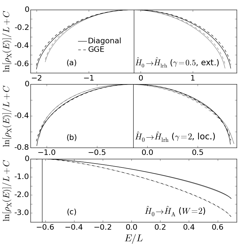
Figure 1: Value of $\ln[\rho_{\mathrm{\scriptscriptstyle D}}(E)]/L$ and $\ln[\rho_{\mathrm{\scriptscriptstyle GGE}}(E)]/L$ computed with the weighted-WLA. The gray curves are obtained with $L=128$, while the black ones with $L=256$. The solid vertical lines are the average energy after the quench, i.e. $\langle\Psi_{0}|\hat{H}|\Psi_{0}\rangle$, for $L=256$. The three panels are obtained starting from the ground states of clean chains and quenching to different disordered Hamiltonians: panel (a) long-range hopping with $\gamma=0.5$ (extended eigenstates), panel (b) long-range hopping with $\gamma=2$ (localized eigenstates) and panel (c) Anderson model with $W=2$. For the computations we used a single disorder realization and, to get a smoother size dependence, the smaller size realization is obtained by cutting an equal amount of sites at the two edges of the larger realization. These distributions are obtained for a single realization of the couplings, but we verified that, for large sizes, the results are self-averaging.

Observe, first, that the distributions $\rho_{\mathrm{\scriptscriptstyle D}}(E)$ and $\rho_{\mathrm{\scriptscriptstyle GGE}}(E)$ shown in Fig. 1 have identical average (denoted by a solid vertical line)

$$\langle\hat{H}\rangle_{\mathrm{\scriptscriptstyle D}}=\int\!\mathrm{d}E\,\rho_{\mathrm{\scriptscriptstyle D}}(E)\,E=\int\!\mathrm{d}E\,\rho_{\mathrm{\scriptscriptstyle GGE}}(E)\,E=\langle\hat{H}\rangle_{\mathrm{\scriptscriptstyle GGE}}\;.$$

This result comes directly from the fact that the energy does not fluctuate in time (i.e., the diagonal energy coincides with the average energy $\langle\Psi_{0}|\hat{H}|\Psi_{0}\rangle$) and GGE fixes the occupation of the fermionic eigenstates in such a way as to exactly reproduce $\langle\Psi_{0}|\hat{H}|\Psi_{0}\rangle$. The form of the two distributions, however, differs considerably, most notably at the extremes of the spectrum, and for the Anderson model case. Let us now consider the fluctuations of the energies in both distributions. In the diagonal ensemble the variance is:

$$\sigma^{2}_{E,\mathrm{\scriptscriptstyle D}}=\int\mathrm{d}E\,\rho_{\mathrm{\scriptscriptstyle D}}(E)\,E^{2}-\langle\hat{H}\rangle_{\mathrm{\scriptscriptstyle D}}^{2}=\langle\hat{H}^{2}\rangle_{\mathrm{\scriptscriptstyle D}}-\langle\hat{H}\rangle_{\mathrm{\scriptscriptstyle D}}^{2}\;,$$ (17)

where the expression on the right-hand side holds only for the Hamiltonian (it would not apply to arbitrary operators, because $(A_{\alpha\alpha})^{2}\neq\langle\alpha|\hat{A}^{2}|\alpha\rangle$). An entirely similar expression applies to the GGE case. Since the energy is an extensive operator, it is reasonable to ask what happens to the fluctuations in the energy-per-site $e=E/L$, which are simply given by $\sigma^{2}_{e,\mathrm{\scriptscriptstyle D}}=\sigma^{2}_{E,\mathrm{\scriptscriptstyle D}}/L^{2}$, and $\sigma^{2}_{e,\mathrm{\scriptscriptstyle GGE}}=\sigma^{2}_{E,\mathrm{\scriptscriptstyle GGE}}/L^{2}$. On pretty general grounds, for quenches of local non-integrable Hamiltonians, it is known [12, 13] that $\sigma^{2}_{e,\mathrm{\scriptscriptstyle D}}\to 0$ in the thermodynamic limit, $L\to\infty$. Indeed, as shown in Fig. 2 both $\sigma_{e,\mathrm{\scriptscriptstyle D}}^{2}$ and $\sigma_{e,\mathrm{\scriptscriptstyle GGE}}^{2}$ decrease to $0$ for $L\to\infty$ for the three considered cases. For our quadratic problems, however, we can say a bit more. First of all, from the explicit expression in Eq. (17) after very simple algebra (mainly using Wick’s theorem), we arrive at:

$$\sigma_{e,\mathrm{\scriptscriptstyle GGE}}^{2}=\frac{1}{L^{2}}\sum_{\mu}\epsilon_{\mu}^{2}n^{0}_{\mu}\left(1-n^{0}_{\mu}\right)\;,$$ (18)

$$\sigma_{e,\mathrm{\scriptscriptstyle D}}^{2}=\sigma_{e,\mathrm{\scriptscriptstyle GGE}}^{2}-\frac{1}{L^{2}}\sum_{\mu_{1}\neq\mu_{2}}\epsilon_{\mu_{1}}\epsilon_{\mu_{2}}\left|G^{0}_{\mu_{1}\mu_{2}}\right|^{2}\;,$$ (19)

where $G^{0}_{\mu_{1}\mu_{2}}\equiv\langle\Psi_{0}|\hat{d}^{\dagger}_{\mu_{1}}\hat{d}_{\mu_{2}}|\Psi_{0}\rangle$ is the $t=0$ one-body Green’s function. The off-diagonal elements of $G^{0}_{\mu_{1}\mu_{2}}$ play here an important role, and the second term in $\sigma_{e,\mathrm{\scriptscriptstyle D}}^{2}$ originates from the fact that, by definition, GGE does not include correlations between different eigen-modes, i.e., $\langle\hat{d}^{\dagger}_{\mu_{1}}\hat{d}_{\mu_{2}}\rangle_{\mathrm{\scriptscriptstyle GGE}}=0$, when $\mu_{1}\neq\mu_{2}$.

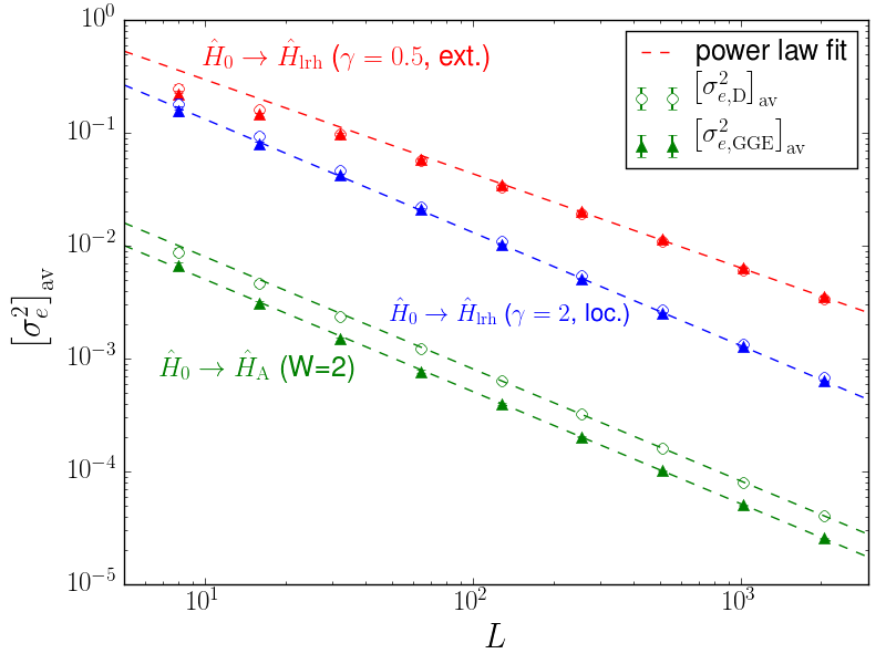
Figure 2: Variances $\sigma^{2}_{e,\mathrm{\scriptscriptstyle D}}=\sigma^{2}_{E,\mathrm{\scriptscriptstyle D}}/L^{2}$ (empty circles) and $\sigma^{2}_{e,\mathrm{\scriptscriptstyle GGE}}=\sigma^{2}_{E,\mathrm{\scriptscriptstyle GGE}}/L^{2}$ (solid triangles) as a function of the size $L$. The data are obtained using the same set of quenches used in Fig. 1 and the values are computed using Eqs. (19). Error bars are calculated by averaging over 20 different realizations of the disorder. The dashed lines are power law fits $\sigma^{2}_{e}\sim L^{-s}$, where $s\approx 1$ for the Anderson case, while, for the quench to $\hat{H}_{\mathrm{lrh}}$, $s\approx 0.82$ when $\gamma=0.5$, and $s\approx 0.95$ when $\gamma=2$. Notice the observable difference between $\sigma^{2}_{e,\mathrm{\scriptscriptstyle D}}$ and $\sigma^{2}_{e,\mathrm{\scriptscriptstyle GGE}}$ when the final eigenstates are localized.

Let us first consider the Anderson model case. Assuming, as done so far, a bounded distribution of disorder, we are guaranteed that a finite bound $\epsilon_{\mathrm{max}}$ exists such that $|\epsilon_{\mu}|\leq\epsilon_{\mathrm{max}}$ for any $L$. With this assumption, it is easy show that $\sigma_{e,\mathrm{\scriptscriptstyle GGE}}^{2}$ has to go to zero at least as $1/L$ for $L\to\infty$. Indeed, the occupation factors appearing in $\sigma_{e,\mathrm{\scriptscriptstyle GGE}}^{2}$ are such that $0\leq n^{0}_{\mu}\left(1-n^{0}_{\mu}\right)\leq 1/4$. Hence:

$$\sigma_{e,\mathrm{\scriptscriptstyle GGE}}^{2}\leq\frac{\epsilon_{\mathrm{max}}^{2}}{L^{2}}\sum_{\mu}n^{0}_{\mu}\left(1-n^{0}_{\mu}\right)\leq\frac{\epsilon_{\mathrm{max}}^{2}}{4L}\;.$$ (20)

The same statement can be made for $\sigma_{e,\mathrm{\scriptscriptstyle D}}^{2}$, because the difference between the two variances has a similar upper bound:

$$|\sigma_{e,\mathrm{\scriptscriptstyle D}}^{2}-\sigma_{e,\mathrm{\scriptscriptstyle GGE}}^{2}|\leq\frac{1}{L^{2}}\sum_{\mu_{1}\neq\mu_{2}}|\epsilon_{\mu_{1}}||\epsilon_{\mu_{2}}|\left|G^{0}_{\mu_{1}\mu_{2}}\right|^{2}\leq\frac{\epsilon_{\mathrm{max}}^{2}}{L^{2}}\sum_{\mu_{1}\neq\mu_{2}}\left|G^{0}_{\mu_{1}\mu_{2}}\right|^{2}\leq\frac{\epsilon_{\mathrm{max}}^{2}}{L}\;,$$ (21)

where we used that $\sum_{\mu_{1}\mu_{2}}\left|G^{0}_{\mu_{1}\mu_{2}}\right|^{2}=N_{\mathrm{F}}\leq L$. Nevertheless, although both $\sigma_{e,\mathrm{\scriptscriptstyle D}}^{2}$ and $\sigma_{e,\mathrm{\scriptscriptstyle GGE}}^{2}$ go to $0$ as $1/L$ for the Anderson model, they do so with a different pre-factor, see Fig. 2 and comments below.

For the quenches to $\hat{H}_{\mathrm{lrh}}$, a bound $\epsilon_{\mathrm{max}}$ for the single-particle spectrum is in principle not defined: one can think of rare realizations in which the hopping is large at arbitrarily large distances, which would give an unbounded distribution of eigenvalues $\epsilon_{\mu}$. Indeed, the behavior of both $\sigma_{e,\mathrm{\scriptscriptstyle D}}^{2}$ and $\sigma_{e,\mathrm{\scriptscriptstyle GGE}}^{2}$ suggest, see Fig. 2, that the power-law approach to $0$ might be slower than $1/L$, i.e., as $L^{-s}$ with $s<1$ (we find $s\approx 0.82$ for the case $\gamma=0.5$ and $s\approx 0.95$ for $\gamma=2$). While this might be a finite-size artifact, we find it intriguing that such deviations are quite clearly seen for quenches to $\hat{H}_{\mathrm{lrh}}$: they might be due to the power-law nature of the hopping integral variance.

Concerning the similarity between $\sigma_{e,\mathrm{\scriptscriptstyle D}}^{2}$ and $\sigma_{e,\mathrm{\scriptscriptstyle GGE}}^{2}$, we observe that the two essentially coincide for the case of a quench to $\hat{H}_{\mathrm{lrh}}$ with extended eigenstates, while there is a small discrepancy for the quench to $\hat{H}_{\mathrm{lrh}}$ with localized eigenstates, and a quite clear different pre-factor in the Anderson model case, $\sigma_{e,\mathrm{\scriptscriptstyle D}}^{2}\sim C_{\mathrm{\scriptscriptstyle D}}/L$ and $\sigma_{e,\mathrm{\scriptscriptstyle GGE}}^{2}\sim C_{\mathrm{\scriptscriptstyle GGE}}/L$ with $C_{\mathrm{\scriptscriptstyle GGE}}<C_{\mathrm{\scriptscriptstyle D}}$. This different pre-factor can be understood by analyzing the term $\sum_{\mu_{1}\neq\mu_{2}}\epsilon_{\mu_{1}}\epsilon_{\mu_{2}}|G^{0}_{\mu_{1}\mu_{2}}|^{2}$ which appears in Eq. (19). In Fig. 3, panel (b), we show the structure of the matrix $|G^{0}_{\mu_{1}\mu_{2}}|^{2}$ for the three quench cases. We divide this matrix into four sectors, one for each sign of the single-particle energies $\epsilon_{\mu_{1}}$ and $\epsilon_{\mu_{2}}$: in two of these quadrants the product $\epsilon_{\mu_{1}}\epsilon_{\mu_{2}}$ is positive (top-right and bottom-left), and in the others is negative. For quenches to $\hat{H}_{\mathrm{lrh}}$ this matrix is almost equally distributed in all the four sectors: the sum $\sum_{\mu_{1}\neq\mu_{2}}\epsilon_{\mu_{1}}\epsilon_{\mu_{2}}|G^{0}_{\mu_{1}\mu_{2}}|^{2}$ has cancellations, leading to $\sigma_{e,\mathrm{\scriptscriptstyle GGE}}^{2}\approx\sigma_{e,\mathrm{\scriptscriptstyle D}}^{2}$ for large sizes. For quenches to $\hat{H}_{\mathrm{A}}$, on the contrary, the matrix $|G^{0}_{\mu_{1}\mu_{2}}|^{2}$ is mainly concentrated in the sectors in which $\epsilon_{\mu_{1}}\epsilon_{\mu_{2}}<0$, leading to $\sigma_{e,\mathrm{\scriptscriptstyle GGE}}^{2}<\sigma_{e,\mathrm{\scriptscriptstyle D}}^{2}$.

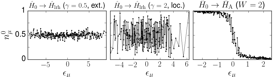
Panel (a)

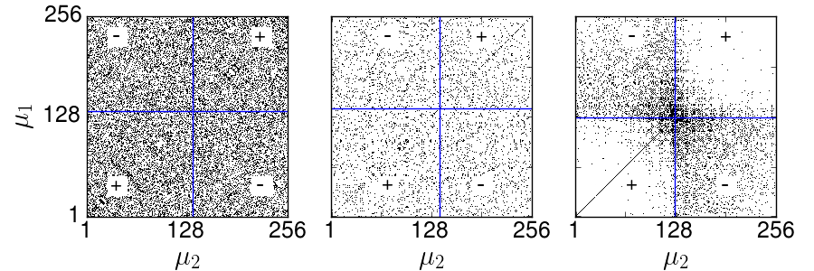
Panel (b)

Figure 3: Panel (a): occupations $n_{\mu}^{0}=\langle\Psi_{0}|\hat{d}_{\mu}^{\dagger}\hat{d}_{\mu}|\Psi_{0}\rangle$ as a function of the single-particle energy $\epsilon_{\mu}$. Panel (b): representation of the matrix $|G^{0}_{\mu_{1}\mu_{2}}|^{2}$. For the diagonal and off-diagonal elements we add a black pixel when the value exceeds their mean value. For the diagonal elements the mean value is $x\equiv\sum_{\mu}(n_{\mu}^{0})^{2}/L$, while for the off-diagonal elements the mean value is $(N_{\mathrm{F}}-xL)/L(L-1)$, where $N_{\mathrm{F}}$ is the number of fermions in the initial state, and we used the relation $\sum_{\mu_{1}\mu_{2}}|G^{0}_{\mu_{1}\mu_{2}}|^{2}=N_{\mathrm{F}}$ (see [31, App. D]). The vertical and horizontal lines indicate the indexes at which the single-particle energies $\epsilon_{\mu_{1}}$ and $\epsilon_{\mu_{2}}$ change sign, and the signs shown in the four quadrants are those of the product $\epsilon_{\mu_{1}}\epsilon_{\mu_{2}}$. For the two panels we used $L=256$ and the same quenches used in Fig. 1 and Fig. 2.

Finally, let us comment on one aspect of the distributions shown in Fig. 1 which can be easily understood from the single-particle occupations shown in Fig. 3. We see that, when the after-quench Hamiltonian is the Anderson model, $\rho_{\mathrm{\scriptscriptstyle D}}(E)$ has both mode (i.e., maximum value) and average very close to the ground state energy: the quench excites mostly the low-energy part of the many-body spectrum. On the contrary, for both the quenches towards $\hat{H}_{\mathrm{lrh}}$, mode and average are almost in the middle of the many-body spectrum; there, indeed, the quench is more dramatic: we are going from the ground state of a chain with nearest-neighbor hopping to a disordered chain with long-range hopping. This is evident by looking at the occupations $n_{\mu}^{0}\equiv\langle\Psi_{0}|\hat{d}^{\dagger}_{\mu}\hat{d}_{\mu}|\Psi_{0}\rangle$ as a function of the single-particle energy $\epsilon_{\mu}$, shown in Fig. 3, panel (a). By definition, only the eigenstates of $\hat{H}_{0}$ with $\epsilon_{\nu}^{0}<0$ are occupied in $|\Psi_{0}\rangle$. The quench to $\hat{H}_{\mathrm{A}}$ only slightly modifies the initial occupations: $n_{\mu}^{0}$, apart for fluctuations due to disorder, goes smoothly from $1$, in the lower part of the single-particle spectrum, to $0$, in the highest part of the spectrum. On the contrary, for the quenches towards $\hat{H}_{\mathrm{lrh}}$, the single-particle spectrum is entirely excited, both the positive and the negative energy part. This explains why, for these quenches, the after-quench energy $\langle\Psi_{0}|\hat{H}|\Psi_{0}\rangle=\sum_{\mu}\epsilon_{\mu}n^{0}_{\mu}$ is near the center of the many-body spectrum.

3.2 Probability distributions of the local density

Let us now consider the local density $\hat{n}_{j}\equiv\hat{c}^{\dagger}_{j}\hat{c}_{j}$, perhaps the simplest one-body observable. For definiteness, we concentrate on $j=L/2$, the center of the chain. It is important to stress that we are going to consider the fluctuations of $\hat{n}_{j}$ before any possible average over the sites $j$: averaging over the sites $j$ an intensive local operator would effectively send to zero the fluctuations in the thermodynamic limit [13], while we will show that, for a fixed $j$, finite fluctuations survive in the thermodynamic limit when the eigenstates are localized, due to disorder.

The diagonal and GGE distributions $\rho_{\mathrm{\scriptscriptstyle D}}(n)$ and $\rho_{\mathrm{\scriptscriptstyle GGE}}(n)$ are now constructed using the matrix elements $n_{\alpha\alpha}\equiv\langle\alpha|\hat{n}_{j}|\alpha\rangle=\sum_{\mu}|u_{j\mu}|^{2}n_{\mu}^{\alpha}$, where $n_{\mu}^{\alpha}=0,1$ are, as before, the single-particle occupations of the eigenstate $|\alpha\rangle$. In Fig. 4 we plot $\ln[\rho_{\mathrm{\scriptscriptstyle D}}(n)]$ and $\ln[\rho_{\mathrm{\scriptscriptstyle GGE}}(n)]$, computed for the three quenches discussed before. The case of a quench to $\hat{H}_{\mathrm{lrh}}$ with $\gamma=2.0$ (localized eigenstates) is quite peculiar. The values that $n$ can assume is actually split in two separated domains, one just above $n=0$ and one just below $n=1$, and the mean value is exactly in the middle, where no values of $n_{\alpha\alpha}$ happen to fall. This is due to the strong spatial localization of the eigenstates. As we show in Fig. 5, at fixed $j$, the value of $|u_{j\mu}|^{2}$ is strongly localized in a single eigenstate $\tilde{\mu}$. This implies that the value $n_{\alpha\alpha}=\sum_{\mu}|u_{j\mu}|^{2}n_{\mu}^{\alpha}$ has a strong jump when we move from a state $|\alpha\rangle$ in which $n_{\tilde{\mu}}^{\alpha}=0$, to the state $|\alpha\rangle$ in which $n_{\tilde{\mu}}^{\alpha}=1$. For the quench to $\hat{H}_{\mathrm{A}}$, with $W=2$, the localization is not strong enough to produce such a gap: we however expect this to happen for larger values of the disorder amplitude $W$.

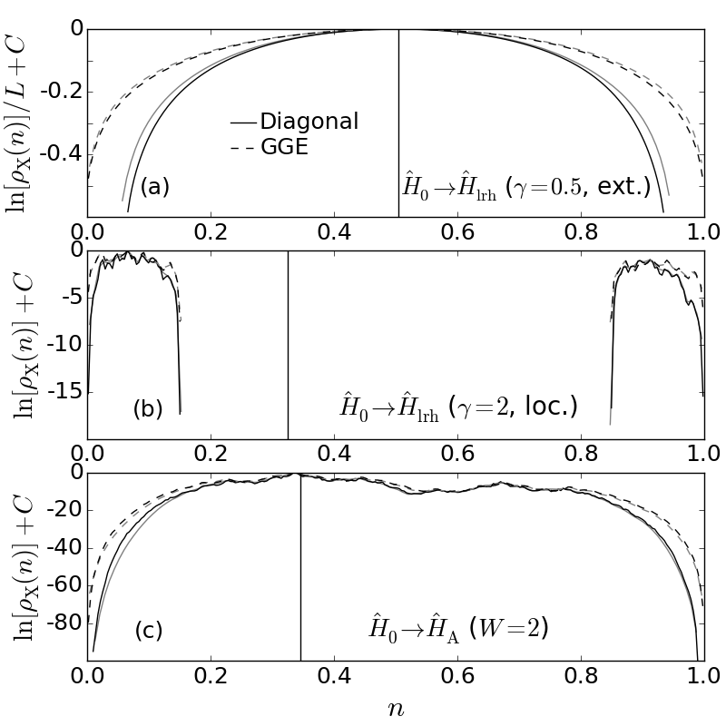
Figure 4: Distributions of the local density $\hat{n}_{j}$ at the center of the chain, $j=L/2$, for the diagonal ensemble and the GGE, and for $L=256$ (black curves) or $L=128$ (gray curves). In panel (a), we plot $\ln[\rho_{\mathrm{\scriptscriptstyle D}}(n)]/L$ and $\ln[\rho_{\mathrm{\scriptscriptstyle GGE}}(n)]/L$, while in panels (b) and (c) $\ln[\rho_{\mathrm{\scriptscriptstyle D}}(n)]$ and $\ln[\rho_{\mathrm{\scriptscriptstyle GGE}}(n)]$. The vertical lines are the diagonal and GGE average of $\hat{n}_{j}$, which coincide for the local density. The three panels are obtained using the same quenches of Fig. 1.

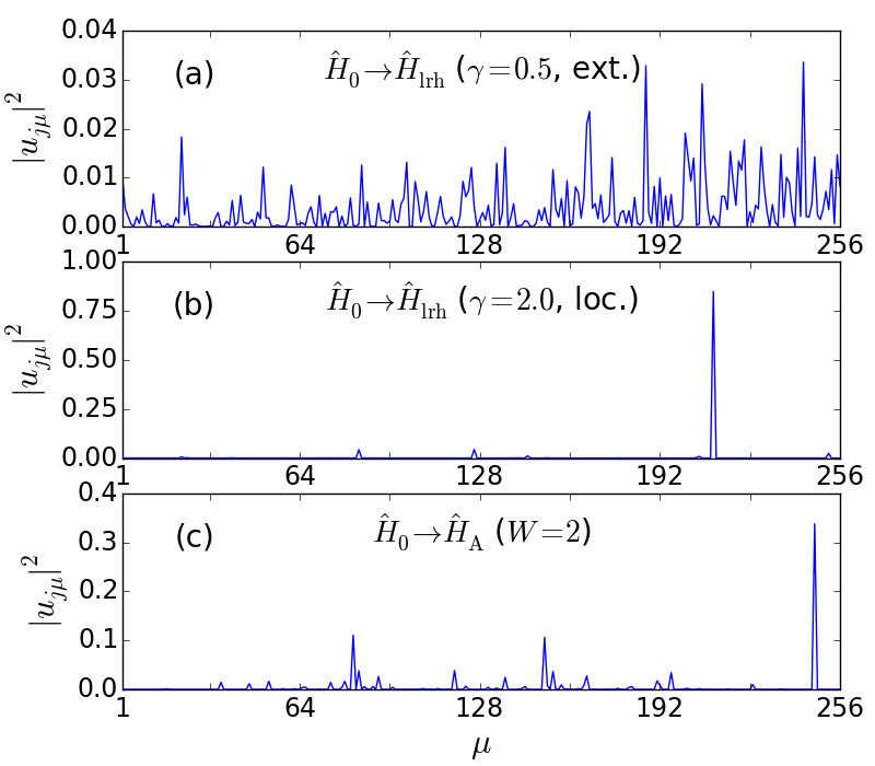
Figure 5: Squared single-particle wavefunction $|u_{j\mu}|^{2}$ as a function of the eigenstates index $\mu$, at fixed site $j=L/2$. We have taken $L=256$ and the three panels are obtained using the same quenches of Fig. 1.

Since $\hat{n}_{j}$ is a one-body operator, the diagonal and GGE averages coincide [11], and therefore, the mean value of the two distributions is the same:

$$\int\!\mathrm{d}n\,\rho_{\mathrm{\scriptscriptstyle D}}(n)\,n=\int\!\mathrm{d}n\,\rho_{\mathrm{\scriptscriptstyle GGE}}(n)\,n\;.$$

We also note that, for this observable, $\hat{n}_{j}^{m}=\hat{n}_{j}$ for any positive integer $m$, and therefore $\langle\hat{n}_{j}^{m}\rangle_{\mathrm{\scriptscriptstyle D}}=\langle\hat{n}_{j}^{m}\rangle_{\mathrm{\scriptscriptstyle GGE}}$. However, this does not allow us to conclude that the two distributions $\rho_{\mathrm{\scriptscriptstyle D}}(n)$ and $\rho_{\mathrm{\scriptscriptstyle GGE}}(n)$ coincide, since, unlike the case of the total energy, we have that, for instance:

$$\int\!\mathrm{d}n\,\rho_{\mathrm{\scriptscriptstyle D}/\mathrm{\scriptscriptstyle GGE}}(n)\,n^{2}\neq\langle\hat{n}_{j}^{2}\rangle_{\mathrm{\scriptscriptstyle D}/\mathrm{\scriptscriptstyle GGE}}\;.$$

The variance of the two distributions can be computed by exploiting again Wick’s theorem. We find that:

$$\sigma_{n,\mathrm{\scriptscriptstyle GGE}}^{2}=\sum_{\mu}\left|u_{j\mu}\right|^{4}n^{0}_{\mu}\left(1-n^{0}_{\mu}\right)$$ (22)

$$\sigma_{n,\mathrm{\scriptscriptstyle D}}^{2}=\sigma_{n,\mathrm{\scriptscriptstyle GGE}}^{2}-\sum_{\mu_{1}\neq\mu_{2}}\left|u_{j\mu_{1}}\right|^{2}\left|u_{j\mu_{2}}\right|^{2}\left|G^{0}_{\mu_{1}\mu_{2}}\right|^{2}\;.$$ (23)

In Fig. 6 we plot $\sigma_{n,\mathrm{\scriptscriptstyle GGE}}^{2}$ and $\sigma_{n,\mathrm{\scriptscriptstyle D}}^{2}$ as a function of size. We see that, in both ensembles, the variances vanish as $1/L$ when quenching to $\hat{H}_{\mathrm{lrh}}$ with $\gamma=0.5$ (extended eigenstates) while they are finite when quenching to $\hat{H}_{\mathrm{A}}$ and to $\hat{H}_{\mathrm{lrh}}$ with $\gamma=2$, i.e., when the final Hamiltonian has localized eigenstates. These results agree with the findings of Ref. [32], who show that, for large $L$, the variance of few-body intensive (but not site-averaged) observables remains finite both in the microcanonical ensemble and in the diagonal ensemble for the Aubry-André model.

From the equation for $\sigma_{n,\mathrm{\scriptscriptstyle GGE}}^{2}$, we see that it is related to an inverse participation ratio (IPR): the sum is over the eigenstates $\mu$, each $\mu$ weighted with the corresponding occupation factor $0\leq n^{0}_{\mu}\left(1-n^{0}_{\mu}\right)\leq 1/4$ depending on the initial state. It is therefore easy to realize that:

$$\sigma_{n,\mathrm{\scriptscriptstyle GGE}}^{2}\leq\frac{1}{4}\sum_{\mu}\left|u_{j\mu}\right|^{4}=\frac{\mathrm{IPR}_{j}}{4}\;,$$ (24)

where the last equality defines the IPR at fixed site $j$. This shows that, whenever the IPR goes to zero, i.e., when the final Hamiltonian has delocalized eigenstates, $\sigma_{n,\mathrm{\scriptscriptstyle GGE}}^{2}$ goes to zero as well. For a final Hamiltonian with localized eigenstates we have instead the opposite: there is at least one eigenstate $\tilde{\mu}$ localized around $j$, and therefore there is a single-particle wavefunction $u_{j\tilde{\mu}}$ which does not vanish in the thermodynamic limit; if the initial occupation $n^{0}_{\tilde{\mu}}$ of this eigenstate is such that $0<n^{0}_{\tilde{\mu}}<1$, then $\sigma_{n,\mathrm{\scriptscriptstyle GGE}}^{2}$ remain finite in the thermodynamic limit.

Concerning $\sigma_{n,\mathrm{\scriptscriptstyle D}}^{2}$, Eq. (23) can be rewritten as:

$$\sigma_{n,\mathrm{\scriptscriptstyle D}}^{2}=\sigma_{n,\mathrm{\scriptscriptstyle GGE}}^{2}-\delta^{2}_{jj}\;,$$ (25)

where $\delta^{2}_{jj}$ denotes the mean squared time-fluctuations of the single-particle Green’s function $G_{j_{1}j_{2}}(t)$ [10]:

$$\delta_{j_{1}j_{2}}^{2}\equiv\lim_{t\rightarrow\infty}\frac{1}{t}\int_{0}^{t}\mathrm{d}t^{\prime}\,\left|\delta G_{j_{1}j_{2}}(t^{\prime})\right|^{2}\;,$$ (26)

$\delta G_{j_{1}j_{2}}(t)\equiv G_{j_{1}j_{2}}(t)-\overline{G_{j_{1}j_{2}}}$ being the time fluctuation with respect to the long-time average $\overline{G_{j_{1}j_{2}}}$. Physically, $\delta_{jj}^{2}$ is the averaged long-time fluctuation of the local density $\hat{n}_{j}=\hat{c}_{j}^{\dagger}\hat{c}_{j}$. In Refs. [10, 11] we have shown that if the final Hamiltonian has extended eigenstates, then $\delta^{2}_{jj}\approx 1/L$ for large sizes, while $\delta^{2}_{jj}$ remains finite when the final Hamiltonian has localized eigenstates. This explains all the features shown in Fig. 6, in particular the clear difference between $\sigma_{n,\mathrm{\scriptscriptstyle D}}^{2}$ and $\sigma_{n,\mathrm{\scriptscriptstyle GGE}}^{2}$ in all cases.

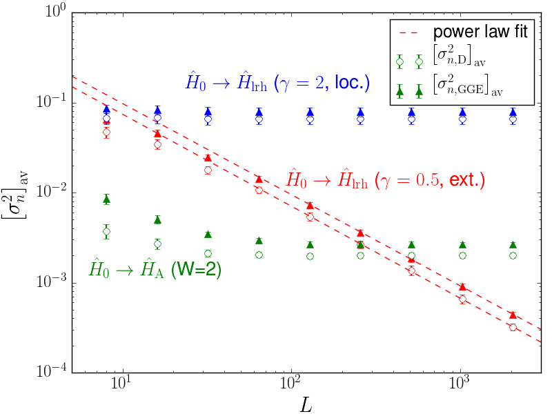
Figure 6: Plot of the variances $\sigma_{n,\mathrm{\scriptscriptstyle D}}^{2}$ (circles) and $\sigma_{n,\mathrm{\scriptscriptstyle GGE}}^{2}$ (triangles) as a function of size. The data are obtained using the same set of quenches used in Fig. 2 and the values are computed using Eq. (23). Error bars are calculated by averaging over 20 different realizations of the disorder. The dashed lines are power-law fits $\sigma^{2}_{n}\sim L^{-s}$, where $s\approx 1$ in both cases.

4 Summary and conclusions

In this paper we have introduced a Monte Carlo method — obtained by a rather natural extension of the Wang-Landau algorithm [19, 20, 21] — which allows to compute quite general weighted distribution functions of the form relevant to quantum quenches, see Eq. (6). We have used this approach to analyze quantum quenches for free-fermion Hamiltonians in presence of disorder. For these systems, thanks to Wick’s theorem, after-quench expectation values and time averages require a modest computational effort, proportional to a power-law of the size $L$ [11]. However, the calculation of full probability distributions — like the diagonal ensemble distribution $\rho_{\mathrm{D}}(A)$, Eq. (3), or the GGE one $\rho_{\mathrm{GGE}}(A)$, Eq. (5) — would still require a sum over an exponential number of terms, hence unfeasible beyond very small sizes.

Although quadratic, hence with an extensive number of conserved quantities, these free-fermion problems are not described by the GGE ensemble whenever the disorder is such that the after-quench eigenstates are localized. More precisely, while the GGE ensemble is known to correctly capture the long-time average of any one-body operator, almost “by construction” [11], it does not capture correlations induced by the spatial localization of the eigenstates. Our study further explored this issue by explicitly calculating and comparing the full probability distributions of both the energy and the local density in the two relevant ensembles.

Concerning the energy, we have explicitly verified that the form of the two distributions for the diagonal and GGE ensembles differs considerably, most notably at the extremes of the spectrum, and for the Anderson model case. More in detail, we have verified that, regardless of the final Hamiltonian, the averaged fluctuations of the energy-per-site, $\left[\sigma_{e,\mathrm{\scriptscriptstyle D}}^{2}\right]_{\mathrm{av}}$ and $\left[\sigma_{e,\mathrm{\scriptscriptstyle GGE}}^{2}\right]_{\mathrm{av}}$, go to zero in the thermodynamic limit, see Fig. 2, in agreement with the general analysis of Refs. [12, 13]. Nevertheless, we find that there is a clearly detectable difference in the two variances when the final Hamiltonian has localized eigenstates.

In addition to the energy, we studied the local density distributions. For this observable, it was already known that, even in presence of disorder and localization, the GGE expectation value coincides with the diagonal average [11], a property true, more generally, for any one-body operator [11]. Our numerical results confirm that even if the averages of $\rho_{\mathrm{D}}(n)$ and $\rho_{\mathrm{GGE}}(n)$ coincide, the two distributions are different when localization is present, with clearly detectable differences already at the level of the variance, see Fig. 6: $\sigma_{n,\mathrm{\scriptscriptstyle GGE}}^{2}$ and $\sigma_{n,\mathrm{\scriptscriptstyle D}}^{2}$ differ by a quantity which represents the averaged long-time fluctuations of the local density [10, 11], which remain finite whenever the final Hamiltonian has localized eigenstates.

Other many-body operators, like density-density correlations, might be analyzed in a similar way. Here, even the average values are not in general well described by the GGE distribution whenever localization is at play [11]: we expect, once again, clearly visible discrepancies between the diagonal and GGE distributions in such cases.

In conclusion, as explained above, the weighted-WLA we have presented circumvents the difficulty associated to the exponentially large Hilbert space to be visited, even when the relevant ingredients entering the distribution — matrix elements and overlap between states — can be calculated quite effectively. In principle, the applicability of the method is not limited to “quadratic fermion problems” of the type we have considered in the paper: If, by Bethe Ansatz, or any other exact technique or even by a suitable quantum Monte Carlo approach, one would be able to calculate matrix elements and overlaps, the method we have illustrated would provide an effective Monte Carlo sampling of the relevant distribution functions.

References

References

- [1] Immanuel Bloch, Jean Dalibard, and Wilhelm Zwerger. Many-body physics with ultracold lattices. Rev. Mod. Phys., 80:885–964, 2008.
- [2] Maciej Lewenstein, Anna Sanpera, Veronica Ahufinger, Bodgan Damski, Aditi Sende, and Ujjwal Sen. Ultracold atoms in optical lattices: mimicking condensed matter physics and beyond. Advances in Physics, 56:243–379, 2007.
- [3] J. M. Deutsch. Quantum statistical mechanics in a closed system. Phys. Rev. A, 43:2046–2049, 1991.
- [4] Mark Srednicki. Chaos and quantum thermalization. Phys. Rev. E, 50:888–901, 1994.
- [5] M. Rigol, V. Dunjko, and M. Olshanii. Thermalization and its mechanism for generic isolated quantum systems. Nature, 452:854–858, 2008.
- [6] Marcos Rigol. Breakdown of thermalization in finite one-dimensional systems. Phys. Rev. Lett., 103:100403, 2009.
- [7] Marcos Rigol. Quantum quenches and thermalization in one-dimensional fermionic systems. Phys. Rev. A, 80:053607, 2009.
- [8] Toshiya Kinoshita and Trevor Wenger and David S. Weiss. A quantum newton’s cradle. Nature (London), 440:900, 2006.
- [9] Anatoli Polkovnikov, Krishnendu Sengupta, Alessandro Silva, and Mukund Vengalattore. Nonequilibrium dynamics of closed interacting quantum systems. Rev. Mod. Phys., 83:863, 2011.
- [10] Simone Ziraldo, Alessandro Silva, and Giuseppe E. Santoro. Relaxation dynamics of disordered spin chains: Localization and the existence of a stationary state. Phys. Rev. Lett., 109:247205, Dec 2012.
- [11] Simone Ziraldo and Giuseppe E. Santoro. Relaxation and thermalization after a quantum quench: Why localization is important. Phys. Rev. B, 87:064201, Feb 2013.
- [12] M. Rigol, V. Dunjko, and M. Olshanii. Thermalization and its mechanism for generic isolated quantum systems. Nature, 452(7189):854–858, 2008.
- [13] Giulio Biroli, Corinna Kollath, and Andreas M. Läuchli. Effect of rare fluctuations on the thermalization of isolated quantum systems. Phys. Rev. Lett., 105:250401, Dec 2010.
- [14] Marcos Rigol, Alejandro Muramatsu, and Maxim Olshanii. Hard-core bosons on optical superlattices: Dynamics and relaxation in the superfluid and insulating regimes. Phys. Rev. A, 74:053616, 2006.
- [15] Marcos Rigol, Vanja Dunjko, Vladimir Yurovsky, and Maxim Olshanii. Relaxation in a completely integrable many-body quantum system: An ab initio study of the dynamics of the highly excited states of 1d lattice hard-core bosons. Phys. Rev. Lett., 98:050405, 2007.
- [16] T. Barthel and U. Schollwöck. Dephasing and the steady state in quantum many-particle systems. Phys. Rev. Lett., 100:100601, Mar 2008.
- [17] Pasquale Calabrese, Fabian H. L. Essler, and Maurizio Fagotti. Quantum quench in the transverse-field ising chain. Phys. Rev. Lett., 106:227203, Jun 2011.
- [18] Miguel A. Cazalilla, Anibal Iucci, and Ming-Chiang Chung. Thermalization and quantum correlations in exactly solvable models. Phys. Rev. E, 85:011133, Jan 2012.
- [19] Fugao Wang and D. P. Landau. Efficient, multiple-range random walk algorithm to calculate the density of states. Phys. Rev. Lett., 86:2050–2053, Mar 2001.
- [20] Fugao Wang and D. P. Landau. Determining the density of states for classical statistical models: A random walk algorithm to produce a flat histogram. Phys. Rev. E, 64:056101, Oct 2001.
- [21] D.P. Landau and F. Wang. Determining the density of states for classical statistical models by a flat-histogram random walk. Computer Physics Communications, 147:674 – 677, 2002.
- [22] R. E. Belardinelli, S. Manzi, and V. D. Pereyra. Analysis of the convergence of the and wang-landau algorithms in the calculation of multidimensional integrals. Phys. Rev. E, 78:067701, Dec 2008.
- [23] Pedro Ojeda, Martin E. Garcia, Aurora Londoño, and N. Y. Chen. Monte carlo simulations of proteins in cages: Influence of confinement on the stability of intermediate states. Biophysical Journal, 96(3):1076 – 1082, 2009.
- [24] Evelina B. Kim, Roland Faller, Qiliang Yan, Nicholas L. Abbott, and Juan J. de Pablo. Potential of mean force between a spherical particle suspended in a nematic liquid crystal and a substrate. The Journal of Chemical Physics, 117(16):7781–7787, 2002.
- [25] M. Müller and J.J. de Pablo. Simulation techniques for calculating free energies. In Computer Simulations in Condensed Matter Systems: From Materials to Chemical Biology Volume 1, volume 703 of Lecture Notes in Physics, pages 67–126. Springer Berlin Heidelberg, 2006.
- [26] B. J. Schulz, K. Binder, M. Müller, and D. P. Landau. Avoiding boundary effects in wang-landau sampling. Phys. Rev. E, 67:067102, Jun 2003.
- [27] M. Gertsenshtein and V. Vasilev. Waveguides with random inhomogeneities and brownian motion in the lobachevsky plane. Theory of Probability & Its Applications, 4(4):391–398, 1959.
- [28] Alexander D. Mirlin, Yan V. Fyodorov, Frank-Michael Dittes, Javier Quezada, and Thomas H. Seligman. Transition from localized to extended eigenstates in the ensemble of power-law random banded matrices. Phys. Rev. E, 54:3221–3230, Oct 1996.
- [29] E. Cuevas, M. Ortuño, V. Gasparian, and A. Pérez-Garrido. Fluctuations of the correlation dimension at metal-insulator transitions. Phys. Rev. Lett., 88:016401, Dec 2001.
- [30] Imre Varga. Fluctuation of correlation dimension and inverse participation number at the anderson transition. Phys. Rev. B, 66:094201, Sep 2002.
- [31] S. Ziraldo. Thermalization and relaxation after a quantum quench in disordered Hamiltonians. PhD thesis, SISSA, Trieste, 2013. Available at: http://www.sissa.it/cm/thesis/2013/Ziraldo.pdf.
- [32] Kai He, Lea F. Santos, Tod M. Wright, and Marcos Rigol. Single-particle and many-body analyses of a quasiperiodic integrable system after a quench. Phys. Rev. A, 87:063637, Jun 2013.