Stimuli-responsive brushes with active minority components: Monte Carlo study and analytical theory

Abstract

Using a combination of analytical theory, Monte Carlo simulations, and three dimensional self-consistent field calculations, we study the equilibrium properties and the switching behavior of adsorption-active polymer chains included in a homopolymer brush. The switching transition is driven by a conformational change of a small fraction of minority chains, which are attracted by the substrate. Depending on the strength of the attractive interaction, the minority chains assume one of two states: An exposed state characterized by a stem-crown-like conformation, and an adsorbed state characterized by a flat two-dimensional structure. Comparing the Monte Carlo simulations, which use an Edwards-type Hamiltonian with density dependent interactions, with the predictions from self-consistent-field theory based on the same Hamiltonian, we find that thermal density fluctuations affect the system in two different ways. First, they renormalize the excluded volume interaction parameter $v_{\mathrm{\tiny bare}}$ inside the brush. The properties of the brushes can be reproduced by self-consistent field theory if one replaces $v_{\mathrm{\tiny bare}}$ by an effective parameter $v_{\mbox{\tiny eff}}$, where the ratio of second virial coefficients $B_{\mbox{\tiny eff}}/B_{\mathrm{\tiny bare}}$ depends on the range of monomer interactions, but not on the grafting density, the chain length, and $v_{\mathrm{\tiny bare}}$. Second, density fluctuations affect the conformations of chains at the brush surface and have a favorable effect on the characteristics of the switching transition: In the interesting regime where the transition is sharp, they reduce the free energy barrier between the two states significantly. The scaling behavior of various quantities is also analyzed and compared with analytical predictions.

I Introduction

Polymer brushes are organic surface layers formed by polymer chains that are grafted at one end to a substrate Lodge ; Milner . Since the thickness of brush layers is typically in the nanometer range, they are interesting for the design of functional surfaces Russell ; R1 ; R2 with applications in a wide variety of areas ranging from colloidal stabilization colloidal_stabilization , lubrication lubrication , controlled friction and adhesion adhesion , anti-fouling antifouling , biocompatibilitybiocompatibility , drug delivery drug_delivery , and smart stimuli-responsive materials R1 . In this respect, multicomponent polymer brushes are particularly promising R1 ; R2 . If the brush chains are covalently bound to the substrate, they cannot phase separate on a global scale, but they can still develop structure on the nanoscale. The resulting brush morphologies are controlled both by the intrinsic properties of the brush, e.g., chemical properties of the chains (compatibility or incompatibility), the grafting densities, the chain lengths, and by the environment-related parameters, such as solvent selectivity, substrate preference, temperature, and the pH. Due to the ability of polymer brushes to selectively respond to environmental stimuli, they can be used to design materials that can reversibly switch/tune their surface properties, e.g., with respect to wettability wettability ; wettability_time , permeability permeability , friction friction , and optical properties optical .

Stimuli-induced phase separation provides the basic mechanism for the change in the brush surface properties depending on which of the two microphases forms the outer part of the brush. A typical example for such a morphology-related switchable surface is a mixed polymer brush with equal amounts of hydrophobic and hydrophilic polymers grafted on a substrate. By treatment of different solvents, the surface composition can change and then the wettability of this material switches wettability ; wettability_time . Morphology change necessarily involves slow highly cooperative chain dynamics and therefore a typical response time turns out to be in the range of several minutes or larger wettability_time .

In a recent letter, we have proposed a new class of brush-based switches Klushin_switch , which rely on a radical conformational change of individual adsorption-active minority chains in an otherwise inert brush.

The selective adsorption driving the transition may arise, e.g., from electrostatic interactions or hydrogen bonding between active groups in the minority chains and the substrate. These active groups can serve as responsive sensors that trigger the switching transition. The most radical change is associated with the end group of the minority chain. In the adsorbed state it resides in close proximity of the substrate deeply buried within the brush, while in the other state it is exposed to the environment. Thus the transition could potentially promote a specific immune-like response. Chemically or biologically active groups can be attached to the free end of the minority chain to serve as practically useful sensors.

Based on theoretical arguments and simple one-dimensional mean-field calculations, we demonstrated that even a small chain length increment of about 10 % produces a sharp transition from the exposed state to the adsorbed state. The transition time is expected to be very short since the free energy barrier between these two thermodynamically stable states is about several $k_{B}T$. A further increase in the minority chain length will lead to sharper transitions, but at the same time to longer transition times due to higher barriers. The strong response of the chain conformation of a minority chain brush_minority_1997 to small variations of its length is related to the recently reported “surface instabilities” in polymer brushes Merlitz1 ; Romeis1 , which can be used to sense solvent quality Merlitz2 ; Romeis2 . In our work, we proposed to use single chains as switches triggered by a change in substrate-polymer interaction. One major benefit of this switch is that it does not involve cooperative rearrangements of many chains, therefore the switching transition is fast as compared to the existing examples in mixed brushes.

The arguments presented in Ref. Klushin_switch rely on several assumptions. First, the presence of the minority chains was taken to have no effect on the surrounding polymer brush. Second, thermal fluctuations of the majority brush component were disregarded.

In the current paper, we present extensive Monte Carlo (MC) simulations of a coarse-grained model for polymer brushes with a single immersed adsorption-active minority chain. To assess the influence of fluctuations separately, we have also performed three-dimensional self-consistent field (SCF) calculations for comparison. We investigate in detail both lateral and longitudinal characteristics of chain conformations and the various characteristics of the transition.

The remainder of the paper is organized as follows: Sec. II outlines the MC model and the simulation scheme. Sec. III presents the MC results for a homogeneous monodisperse brush and comparison with the established analytical SCF theory, and analyzes the dependence of the renormalized virial coefficient on the effective interaction range. Sec. IV presents a more detailed derivation of the theory for the adsorption-active minority chain sketched in Ref. Klushin_switch . In Sec. V the main results of the MC simulations are presented and discussed. This section also compares MC and 3-d SCF calculations with the emphasis on fluctuation effects. A general discussion is given in the final section VI.

II MC simulation model

In the simulation community, a variety of numerical methods have been developed and used to investigate polymer brush systems, ranging from molecular dynamics MD1 , dissipative particle dynamics DPD1 , and Monte Carlo (MC) simulations MC1 ; MC_CG ; MC3 ; MC4 ; MC5 to numerical self-consistent field (SCF) calculations lattice_SCF ; SCF2 ; SCF3 ; SCF4 ; SCF5 ; SCF6 . The present study mainly relies on MC simulations, while for comparison we also present results obtained from 3-d SCF theory. The MC simulation model and scheme are described as follows, and the detailed description of SCF method is shown in the Appendix.

In the MC simulations, we adopt a coarse-grained off-lattice model first proposed by Laradji et al MC_CG . In this approach, a particle-based representation of the polymers is combined with an Edwards type Hamiltonian EdwardsType1 ; EdwardsType2 , which defines non-bonded interactions in terms of local monomer densities. Compared to the more commonly used coarse-grained polymer models with hard-core monomer interactions, the Laradji model has two advantages: First, it can be simulated very efficiently, since the explicit evaluation of pair interactions is often the most time consuming part in a simulation. Second, it uses soft potentials, hence equilibration times are comparatively short. The model does not account for packing effects and for topological constraints (which may restrict the conformational phase space for strongly adsorbed, quasi-two dimensional polymers). However, these are not in the focus of the present study.

Specifically, the model system is a monodisperse brush in a good solvent containing a single minority chain in a volume $V=L_{x}\cdot L_{y}\cdot L_{z}$. We use periodic boundaries along $x$ and $y$ directions, while impenetrable boundary walls are placed at $z=0$ and $z=L_{z}$. Polymer chains are modelled by the discrete Gaussian bead-spring model with spring constant $\frac{3k_{B}T}{2a^{2}}$, where $a$ is the statistical bond length, $k_{B}$ is the Boltzmann constant, and $T$ the temperature. We will use $a$ as the basic length unit, and $k_{B}T$ as the energy unit. All chains are attached to a substrate placed at $z_{0}$ at one end, where $z_{0}$ is chosen smaller than $a$. The impenetrable wall at $z=0$ exerts an attractive potential to all minority chain beads with strength $\varepsilon$ in a range of $0\leqslant z\leqslant a$. There is no explicit solvent in the model and all the relevant interactions in the good solvent case are represented through an effective excluded volume potential between monomers (beads). The Edwards type Hamiltonian of the system reads

$$\beta\mathcal{H} = \frac{3}{2a^{2}}\sum_{\alpha=1}^{n_{b}}\sum_{j=1}^{N_{b}-1}\big{(}\mathbf{R}_{\alpha j}-\mathbf{R}_{\alpha,j-1}\big{)}^{2}$$ (1)

$$+ \frac{3}{2a^{2}}\sum_{j=1}^{N-1}\big{(}\mathbf{R}_{0j}-\mathbf{R}_{0,j-1}\big{)}^{2}$$

$$+ \frac{v_{\mathrm{bare}}}{2}\int d\mathbf{r}\hat{\rho}_{t}^{2}(\mathbf{r})+\int d\mathbf{r}U_{\mathrm{ads}}(\mathbf{r})\hat{\rho}_{m}(\mathbf{r}),$$

where $\beta\equiv 1/k_{B}T$, $\mathbf{R}_{\alpha j}$ denotes the position of the $j$-th bead in the $\alpha$-th chain (the minority chain has the index $\alpha=0$), $n_{b}$ is the total number of brush chains, $\hat{\rho}_{m}$ denotes the local density of minority chain monomers, $\hat{\rho}_{m}=\sum_{j}\delta(\mathbf{r}-\mathbf{R}_{0j})$, and $\hat{\rho}_{t}\equiv\hat{\rho}_{b}+\hat{\rho}_{m}$ the total density of monomers with $\hat{\rho}_{b}\equiv\sum_{\alpha=1}^{n_{b}}\sum_{j}\delta(\mathbf{r}-\mathbf{R}_{\alpha j})$ being the local density of brush monomers. (Here and in the following, the subscript $b$ will be used to denote the brush chains, and $m$ will denote the minority chain.) The first two terms in the Hamiltonian describe the Gaussian stretching energy (bonded interactions) between two neighboring monomers in the same chain. The third term represents the non-bonded effective interactions between polymer beads. For a good solvent the excluded volume parameter $v_{\mathrm{bare}}$ is larger than zero. The fourth term describes the adsorption between the substrate and the minority beads with a step-like adsorption potential,

$$U_{\mathrm{ads}}(\mathbf{r})=\left\{\begin{array}[]{cc}-\varepsilon,&0\leqslant z\leqslant a\\ 0,&\mathrm{otherwise}\end{array}\right.$$ (2)

In the MC simulations, local densities are extracted from the position of the beads by using the Particle-to-Mesh technique Particle_Mesh , which provides a way for the smoothing of density operators. In the present work we use the zeroth order scheme. The system is divided into cubic cells of size $b^{3}$ whose centers define the grid points, and the local densities evaluated by counting the total number of beads in the corresponding cells divided by the cell volume, are defined at these grid points. The smoothed monomer densities for the minority chain and brush chains are denoted as $\rho_{m}$ and $\rho_{b}$, respectively. This implies that two beads interact only when they are in the same cell, and thus the size of the cell is indirectly linked to the interaction strength of non-bonded interactions. Higher order schemes are conceivable, but computationally more expensive. After the density operators are smoothed over the cell volume, the Hamiltonian acquires the familiar form used in the SCF theory Hybrid_PF , hence SCF calculations and MC simulations can be compared directly.

In the present study, the brush chain length is fixed at $N_{b}=100$. In most MC of calculations we choose the excluded volume parameter $v_{\mathrm{bare}}=1$ which would correspond to a Flory-Huggins parameter $\chi=0$ in an explicit solvent solution (athermal solvent condition), and the size of the averaging cell is taken $b=1$. We model relatively dense monodisperse polymer brushes in good solvent with the surface grafting density $\sigma=0.1,\ 0.2,\ 0.3$, with the corresponding overlap parameters $\sigma R_{gb}^{2}\simeq 2,\ 3,\ 5$, where $R_{gb}$ is the mean radius of gyration for an ideal brush polymer. The grafting points of the chains on the substrate were fixed on a regular square lattice.The system size was chosen $L_{x}=40$, $L_{y}=40$, and $L_{z}=100$ in most cases. To assess the influence of finite-size effects, we have also carried out simulations of larger systems with size $L_{x}=60$, $L_{y}=60$, and $L_{z}=100$ for selected parameter values. The results were identical within the error.

MC simulations book_simulation were carried out according to the standard Metropolis criterion. At every MC update, we try to move the position of one chosen monomer to a new position with a distance in space comparable to the bond length. This trial move results in an energy change including the bonded energy and non-bonded energy, and it is accepted or rejected according to the Boltzmann probability in the usual way. In all the simulations $3\times 10^{5}$ MC steps per monomer were performed to equilibrate the system, and another $3\times 10^{5}$ MC steps to extract statistical averages. In order to get good statistics sampling for

the single minority chain, an additional $10^{8}$ MC steps per monomer updating the minority chain monomers were performed during the process of evaluating statistical averages. Final statistical quantities were obtained by averaging the results from 48 separate independent MC runs.

Figure 1: Monomer density profiles for pure brushes at grafting density $\sigma=0.1$(a) and $\sigma=0.3$(b) from MC simulations obtained with interaction cells of different size $b$ as indicated.

III Homogenous brush and renormalization of the second virial coefficient

We first analyze the simulation results for homogenous monodisperse brushes which are very well understood. In contrast to common MC polymer models our model contains an additional free parameter, the cell size $b$, defining the averaging volume for the local density operator, and the excluded volume parameter $v_{\mathrm{bare}}$. Fig. 1 shows the density profiles of homogeneous brushes with two different grafting densities $\sigma=0.1$ and $\sigma=0.3$, and various values of the averaging cell size $b$. It is clear that the choice of cell size has a pronounced effect on the brush density profile. To rationalize this effect we turn to the analytical SCF theory developed over 20 years ago critical_adsorption ; Alexander ; de_Gennes ; Zhulina ; Milner_analytical and subsequently verified by simulations and experiments.

Within the second virial approximation for good solvent conditions and assuming Gaussian elasticity for the chains, the density profile $\rho_{b}(z)$ has a parabolic form

$$\rho_{b}(z)=\frac{3\pi^{2}}{8v_{\mathrm{eff}}N_{b}^{2}}(H^{2}-z^{2})$$ (3)

where the brush height is $H=(4v_{\mathrm{eff}}\sigma/\pi^{2})^{1/3}N_{b}$, and $v_{\mathrm{eff}}$ an effective interaction parameter. Gaussian elasticity is an important ingredient in the analytical theory and the fact that the MC simulation model is also based on a Hamiltonian with a Gaussian term describing chain connectivity allows a more direct comparison. It is known that corrections due to finite chain extensibility become important for dense grafting, but this is outside the scope of the present paper. On the other hand, modifications of the chain elasticity due to the excluded volume effects are naturally taken into account by our MC simulations. The mean-field potential associated with the density, profile, $V_{b}(z)=v_{\mathrm{eff}}\rho_{b}(z)$ is also parabolic

$$V_{b}(z)=V_{0}-\frac{3\pi^{2}z^{2}}{8N_{b}^{2}}$$ (4)

where $V_{0}=\frac{3}{2}(\pi v_{\mathrm{eff}}\sigma/2)^{2/3}$ is the potential at the grafting surface. According to the theory (see for example Milner_analytical ), the brush density profiles evaluated for the same model at different values of $\sigma$ and $N_{b}$ should collapse in the rescaled coordinates $\frac{\rho_{b}(z)}{\sigma^{2/3}}$ vs $\frac{z}{\sigma^{1/3}N_{b}}$ with one adjustable parameter related to the interaction parameter $K=H/(\sigma^{1/3}N_{b})=(4v_{\mathrm{eff}}/\pi^{2})^{1/3}$

$$\frac{\rho(z)}{\sigma^{2/3}}=\frac{3}{2K^{3}}\left[K^{2}-\left(\frac{z}{\sigma^{1/3}N_{b}}\right)^{2}\right]$$ (5)

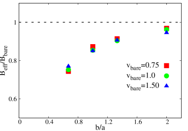
Figure 2: Density profile of polymer brushes (a) in rescaled coordinates $\rho_{b}(z)/\sigma^{2/3}$ vs $z/(\sigma^{1/3}N_{b})$ calculated by MC simulations with $v_{\mathrm{bare}}=1$ for $N_{b}=50,100,200$ and different grafting densities $\sigma=0.1,\ 0.2,\ 0.3$. Dashed line shows the best fit to Eq. (5), corresponding to $K=0.68$. Panel (b) shows the dimensionless ratio $B_{\mathrm{eff}}/B_{\mathrm{bare}}$ as a function of $b/a$ with $B=\frac{1}{2}b^{3}(1-{\rm e}^{-v/b^{3}})$ for different $v_{\mathrm{bare}}$. These points are calculated from $K$ obtained from the best fitting curves at fixed chain length $N_{b}=100$.

The rescaled MC density profiles with $\sigma=0.1,\ 0.2,\ 0.3$ and $N_{b}=50,\>100,\>200$ are presented in Fig. 2, for a specific choice of the averaging cell size, $b=1$ and the “bare” excluded volume parameter $v_{\mathrm{bare}}=1$ . The quality of the collapse is good, and one can extract the value of the effective interaction parameter $v_{\mathrm{eff}}=0.776$, which differs from $v_{\mathrm{bare}}$. The same procedure was repeated for several other values of the $b$ parameter, and different bare excluded volume parameters $v_{\mathrm{bare}}$. To evaluate the difference between $v_{\mathrm{eff}}$ and $v_{\mathrm{bare}}$, we calculate the corresponding exact second exact virial coefficient in the simulation model, taking into account the finite grid size $b$. For given interaction parameter $v$, it is given by $B=\frac{1}{2}b^{3}(1-\mathrm{e}^{-v/b^{3}})$. The ratio $B_{\mathrm{eff}}/B_{\mathrm{bare}}$ for the best fit values of $v_{\mathrm{eff}}$ are plotted as a function of $\frac{b}{a}$ in Fig. 2. The data for different values of $v_{\mathrm{bare}}$ collapse nicely.

We conclude that the renormalization effect can be presented in terms of a dimensionless ratio $\frac{B_{\mathrm{eff}}}{B_{\mathrm{bare}}}$, which is a universal function of a single dimensionless parameter $\frac{b}{a}$ (or, equivalently, $b\sqrt{N}/R_{g}$). Universality in this context does not mean a broad class of different models but rather that other model parameters, such as $\sigma$ and $N_{b}$ do not enter explicitly. It is clear from Fig. 2 that at cell size $b/a=2$ or larger, the curve saturates and $v_{\mathrm{eff}}$ approaches the bare value. Hence the system approaches mean-field behavior if the interaction range $b$ of the monomers becomes large, as one would expect. At smaller $b/a$, local monomer correlations become important and renormalize the effective interaction parameter. Renormalization of monomer interaction parameters has also been observed in Edwards-type simulations of polymer melts Particle_Mesh .

IV Minority chain in a brush: theoretical background

The theory was briefly sketched in Ref. Klushin_switch . In this section, we present it in more detail. We consider a relatively dense monodisperse polymer brush in a good solvent containing a single surface-active minority chain. The length of the minority chain is denoted as $N$, while the length of the brush chain is denoted as $N_{b}$. The minority chain and the brush chains are chemically different and have different interactions with the substrate, i.e., the substrate adsorbs minority chain monomers with strength $\varepsilon$, while it is neutral to the brush chain monomers. Both the minority and the majority chains are flexible with the same statistical Kuhn length $a$ which is taken as the unit length; the excluded volume parameter is also the same for both chain types and is positive corresponding to good solvent conditions. This is fully consistent with the MC model.

We treat the inter- and intrachain interactions in the mean-field approximation and neglect the back effect of the change in the minority chain conformation on the surrounding brush. Hence, the conformation of a minority chain is affected by a fixed mean-field potential profile consisting of the repulsive contribution determined by the brush density and a short-ranged attraction due to the solid substrate. The minority chain itself is described by an ideal continuum model, since intrachain excluded volume effects are screened out considerably within the brush thickness.

The analytical description of the minority polymer chain is based on the continuum approach. The Green’s function $G(z,N)$, i.e. the total statistical weight of the minority chain grafted at the substrate ($z_{0}=0$) as a function of the free end position, $z$, is a solution of the Edwards equation

$$\frac{\partial G(z,s)}{\partial s}=\frac{1}{6}\frac{\partial^{2}G(z,s)}{\partial z^{2}}-V(z)G(z,s)$$ (6)

taken at $s=N$, with the initial condition $G(z,0)=\delta(z)$. The total potential $V(z)=V_{b}(z)+V_{\mathrm{ads}}(z)$, where $V_{\mathrm{ads}}(z)$ is the adsorption attraction potential, and $V_{b}$ is the mean-field brush potential given by Eq. (4). The adsorption potential $V_{\mathrm{ads}}(z)$ is described in the analytical SCF approach as an attractive pseudopotential $V_{\mathrm{ads}}(z)\propto-c\delta(z)$ where $c$ is the adsorption interaction parameter in the continual model. This parameter was introduced by de Gennes de_Gennes_boundary to replace the real adsorption potential through the boundary condition $[G(z,s)]^{-1}\frac{\partial G(z,s)}{\partial z}\big{|}_{z=0}=-c$. Close to the substrate, $z\ll H$, the brush potential changes very little, $V_{b}(z)\simeq V_{0}=\kappa\sigma^{2/3}$ where $\kappa=\frac{3}{2}(\pi v_{\mathrm{eff}}/2)^{2/3}\simeq 1.71$ is a shorthand notation for the numerical coefficient

The adsorbed state is thus approximately described by the standard Green’s function modified by the potential $V_{0}$ brush_minority

$$G_{\mathrm{ads}}(z)=2ce^{N(-V_{0}+c^{2}/6)-cz}.$$ (7)

Integration over $z$ gives the partition function

$$Q_{\mathrm{ads}}=2e^{N(-V_{0}+c^{2}/6)}$$ (8)

In order to connect this expression to the MC model we note that $c^{2}/6$ has the meaning of the negative free energy of adsorption per segment (the chemical potential) in an asymptotically long chain, i.e., $\mu=c^{2}/6$. When comparing the actual brush density profile with the theoretical parabolic shape, one concludes that the pseudopotential must account for the combined effect of the actual adsorption potential (a step of unit width with energy $\varepsilon<0$) and the short-range depression in the brush density near the wall. It is known that for weak adsorption, the free energy per monomer is determined by the crossover exponent $\phi:\mu\sim(\varepsilon-\varepsilon_{c})^{1/\phi}$. For an ideal chain, $\phi=1/2$ while the value for a chain with excluded volume was a subject of extensive investigations and prolonged debates Grassberger ; Klushin_adsorption . For any practical purposes, the adsorption of relatively short chains is very accurately described by the ideal value $\phi=1/2$. Here, for weak adsorption, we adopt the expression

$$\mu(\varepsilon)=\alpha(\varepsilon-\varepsilon_{c})^{2}$$ (9)

where $\alpha$ and $\varepsilon_{c}$ are model-dependent constants to be extracted from the MC data. It is also known that at stronger adsorption, the free energy deviates from Eq. (9), and for very large $\varepsilon$, it can simply be estimated as $\mu=\varepsilon-\mathrm{const}$, where the constant shift is given by the limiting entropy difference per monomer between the coil and the fully adsorbed state.

The state with the free end exposed at the brush edge has no contacts with the surface. Hence the Green’s function is given by the known solution of the Edwards equation for a purely parabolic potential and a neutral solid surface brush_minority_1997

$$G_{\mathrm{ex}}(z,N)=\frac{\pi}{2}\left[\frac{3}{N_{b}\sin\Big{(}\frac{\pi N}{2N_{b}}\Big{)}}\right]^{3/2}ze^{-\frac{3\pi}{4N_{b}}\cot\big{(}\frac{\pi N}{2N_{b}}\big{)}z^{2}}.$$ (10)

For longer minority chains, $N>N_{b}$, the Green’s function of Eq. (10) shows unlimited monotonic increase with $z$ since the solution refers to a potential extending to infinity and to an infinitely extendable Gaussin chain. In a realistic situation the minority chain does not make excursions well beyond $z=H$. To account for this fact we truncate $G_{\mathrm{ex}}(z,N)$ at $z=H$. If minority chains are just slightly longer $\Delta\equiv N-N_{b}\ll N_{b}$, (which is the situation of interest in this paper), the Green’s function simplifies to

$$G_{\mathrm{ex}}(z,N)=\left\{\begin{array}[]{cc}\frac{\pi}{2}\Big{(}\frac{3}{N_{b}}\Big{)}^{3/2}ze^{V_{0}\Delta(\frac{z}{H})^{2}},&z\leqslant H\\ 0,&z>H\end{array}\right..$$ (11)

This gives the partition function

$$Q_{\mathrm{ex}}=\frac{2}{\pi\Delta}(3N_{b})^{1/2}e^{V_{0}\Delta}$$ (12)

assuming $e^{V_{0}\Delta}\gg 1$. Eqs (8) and (12) clearly show that in the limit of $N_{b}\to\infty$, $\sigma=\mathrm{const}$, $\frac{N-N_{b}}{N_{b}}=\mathrm{const}$ the free energies of the two states are extensive and switching become a classical first-order phase transition.

Based on this analytical approach, the transition properties between the adsorbed state and exposed state can be investigated. For example, one could define the transition point as the condition $Q_{\mathrm{ads}}(c^{*})=Q_{\mathrm{ex}}$. Omitting logarithmic correlations this gives $\mu^{*}=V_{0}\frac{\Delta}{N}$. Under the condition $U\frac{\Delta}{N}\ll 1$ one can use the asymptotic expression Eq. (9) to obtain the adsorption energy at the transition

$$-\varepsilon^{*}=-\varepsilon_{c}+(\kappa/\alpha)^{1/2}\sigma^{1/3}\Big{(}\frac{\Delta}{N}\Big{)}^{1/2}$$ (13)

For larger grafting densities and chain length differences one expects deviation from the scaling form of of Eq. (13), since the quadratic dependence of $\mu(\varepsilon)$ may have a limited range. In the extreme case of a very long minority chain, $N\gg N_{b}$, the transition point satisfies the condition $\mu^{*}=V_{0}$. Since the mean-field potential $V_{0}$ is in the range $V_{0}\sim 0.36-0.8$, the limiting value of $\varepsilon^{*}$ remains of order 1.

The sharpness of the transition is characterized by the width of the adsorption parameter change, $\delta\varepsilon$, sufficient to produce a reliable switching from the adsorbed state with the average distance of the free end of the minority chain $Z_{\mathrm{end}}\ll H$ to the exposed state with $Z_{\mathrm{end}}\simeq H$: $\delta\varepsilon=(\frac{1}{H}\frac{dZ_{\mathrm{end}}}{d\varepsilon})^{-1}$ where the derivative is evaluated at the transition point itself. A standard recipe for a two-state model two_state_model gives $\delta\varepsilon=(\frac{1}{4}\frac{d\ln Q_{\mathrm{ads}}}{d\varepsilon})^{-1}\big{|}_{\varepsilon=\varepsilon^{*}})^{-1}$ which combined with Eq. (8) results in

$$\delta\varepsilon=\frac{2}{\kappa}(\kappa/\alpha)^{1/2}\sigma^{-1/3}(N\Delta)^{-1/2}$$ (14)

Finally, the switching time is essentially determined by the barrier separating the two relevant states. Hence we estimate the barrier height at the transition point, $U_{\mathrm{barrier}}$, in terms of the change in the Green’s function of the exposed state, $U_{\mathrm{barrier}}=\ln\frac{G_{\mathrm{ex}}(z=H)}{G_{\mathrm{ex}}(z=z_{\mathrm{barrier}})}$. It follows from Eq. (11) that up to a numerical coefficient close to unity

$$U_{\mathrm{barrier}}\sim V_{0}\Delta\sim\kappa\sigma^{2/3}\Delta$$ (15)

V Simulation Results and discussion

V.1 Adsorbed and exposed conformations of the minority chain

Fig. 3 shows typical simulation snapshots of a brush containing a minority chain $N=120$ (monomers) in an exposed and an adsorbed state. There is a substrate surface below and a virtual surface above showing the brush height $H$. As can be seen a small fraction of monomer units are located above $H$. These monomers form a tenuous brush exterior. The minority chain is shown in green color. It is longer than the majority brush chains with $N_{b}=100$. We characterize the length of the minority chain by a parameter $\Delta=N-N_{b}$ (In the snapshot, $\Delta$ is given by $\Delta=20$). The minority chain in the exposed state has a stem-crown-like conformation.

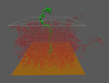
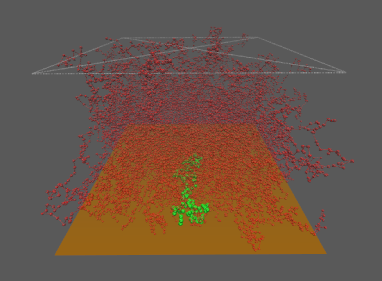
Figure 3: Simulation snapshots of a polymer brush with $N_{b}=100$ and grafting density $\sigma=0.1$ containing a minority chain with $N=120$ in the exposed state (a) at $\varepsilon=0$ and the adsorbed state (b) at $\varepsilon=-0.7$. The minority chain beads are colored green, while the brush chain beads are colored red and made transparent. Brush height $H$ is shown by empty square above for orientation.

The main features of the snapshot can be also seen in Fig. 4 where the longitudinal monomer density profiles are shown for minority chains with different $\Delta$ in the exposed state at $\varepsilon=0$ (panel a), and in the adsorbed state at $\varepsilon=-0.7$(panel b). The density profile of a homogeneous brush is also shown, and for comparison both profiles are normalized in the same way. It is clear that at $\varepsilon=0$ and $\Delta=0$ the minority chain is identical to brush chains. For longer minority chains, $\Delta>0$, the density profile deviates from a parabolic, monotonically decreasing form (apart from a narrow depletion layer near the substrate) shape. It is well understood that the standard parabolic shape is due to a specific very broad end-monomer distribution. “Partial” density profiles produced by chains with a given end position are initially increasing with $z$ with a subsequent sharp drop. Only after averaging over end positions one obtains the actual density profile. The most pronounced effect is observed for the longest minority chain with $\Delta=20$. The profile can be understood if we take chain conformations with the end-monomer positioned on average close to $z=H$ (shown by the vertical dashed line) with a typical fluctuation of a few monomer lengths ($\sim 5).$ For shorter minority chains the average end-hight is below $H$ and the fluctuations are relatively larger, which makes the difference to the majority chains less dramatic. In the strongly adsorbed state the density profile exponentially decreases with $z$ and is insensitive to $\Delta$, see Fig. 4.

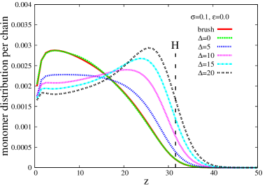
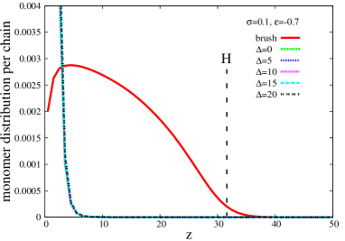
Figure 4: Longitudinal monomer density profiles of minority chains of different length $N=N_{b}+\Delta$ in the exposed state at $\varepsilon=0.0$ (a), and in the adsorbed state at $\varepsilon=-0.7$ (b) as obtained from MC simulations. The brush parameters are $N_{b}=100$ at $\sigma=0.1$. The density profile of the brush chain normalised to unity with is shown for comparison by solid red line. Brush height $H\approx 32$ is shown by vertical dashed line.

Even though the minority chains are highly dilute, they perturb the brush locally. Furthermore, the minority chain itself of course has lateral structure. Fig. 5 shows the lateral distribution of the end monomer $P_{xy}(r)$ as a function of the in-plane radial distance $r=\sqrt{x^{2}+y^{2}}$ from the grafting point for different adsorption energies $\varepsilon$ at grafting density $\sigma=0.2$ and chain length $N=120$. Here $P_{xy}(r)$ was obtained by counting how often the minority chain end was located in a cylindrical shell ranging from $r$ to $r+\Delta r$ and dividing this by the volume of the shell and the total sampling number. The thickness of the shell was chosen as $\Delta r=1$. The results for $\varepsilon=0$ in Fig. 5 show that $P_{xy}(r)$ exhibits Gaussian behavior for nonadsorbing chains. With increasing adsorption strength, the distribution becomes broader, and a depletion region develops close to $r=0$: Chain ends are pushed away from the area close to the grafting point, due to the fact that this area is already covered by adsorbed monomers. This is also shown by the radial distribution density $P_{r}(r)=2\pi rP_{xy}(r)$, which gives the probability to find the free end of the minority chain located at distances ranging from $r$ to $r+\Delta r$ with $\Delta r=1$. At strong enough adsorption the maximum of $P_{r}(r)$ moves towards larger values of $r$ since the flattened adsorbed state dominates (Fig. 5, inset).

Figure 5: Lateral distribution of the free end of the minority chain as a function of radial (in-plane) distance from the grafting point $r$ for $\sigma=0.2$, $N=120$, and different adsorption strengths as indicated. The inset shows the lateral probability given by $P_{r}=2\pi rP_{xy}(r)\Delta r$, where $\Delta r$=1. The data are obtained by MC simulations

Figure 6: Lateral size of the minority chain $R_{\|}$ defined as $R_{\|}=\sqrt{R^{2}_{gx}+R^{2}_{gy}}$ vs the adsorption strength for $\sigma=0.10$ and different minority chain lengths. The data are obtained by MC simulations

To measure more quantitatively how the minority chain extends in the lateral direction, we calculate the parallel root-mean-squared radius of gyration defined as $R_{\|}=\sqrt{R_{gx}^{2}+R_{gy}^{2}}$, where $R_{gx}$ and $R_{gy}$ are the mean-square radius of gyration of the minority chain in the $x$ and $y$ directions, separately.

Fig. 6 shows $R_{\|}$ as a function of the adsorption strength at $\sigma=0.1$ for different minority chain lengths. From these curves it can be seen that the lateral size of the minority chain remains almost unchanged up to $\varepsilon\sim-0.4$, and then starts to increase, which is another signature of the conformational transition from the desorbed to the adsorbed state. Fig. 7 shows the lateral size of the minority chain in the exposed state with $\varepsilon=0$ and in a strongly adsorbed state with $-\varepsilon=0.7$, as a function of the minority chain length for several grafting densities. In both the exposed state and the adsorbed state, $R_{\|}(N)$ is consistent with a power law. The best fit for the exposed state ($\varepsilon=0$) gives $R_{\|}\propto N^{\nu_{e}}$, with $\nu_{e}\thickapprox 0.55$, which is larger than the Flory exponent expected for ideal chains ($\nu=0.5$), and smaller than that expected for free chains in a good solvent ($\nu=0.588$). This can be understood since part of the chain well within the brush experiences semi-dilute conditions with screened excluded volume interactions while the part near the tenuous brush exterior is swollen. As one increases the grafting density at fixed length, the lateral size of the exposed chain decreases. This has two reasons: First, the brush thickens with increasing grafting density, and consequently the fraction of swollen minority chain part outside the brush (the crown) decreases. Second, the monomer density inside the (semi-dilute) brush increases, which leads to a stronger screening of excluded volume interactions and a decrease of lateral swelling of the inner part of the minority chain (the stem). According to Fig. 6, the shrinking does not depend noticeably on the chain length $\Delta=N-N_{b}$ between minority chain and brush chains, i.e. , on the size of the crown. Hence we conclude that the second effect is probably dominant.

For strongly adsorbed chains ($-\varepsilon=0.7$), we find a relation $R_{\|}\propto N^{\nu_{a}}$, with $\nu_{a}\thickapprox 0.73$, which is close to the Flory exponent for two dimensional self-avoiding chains ($\nu=0.75$). In the strongly adsorbed state the lateral extension is almost insensitive to the grafting density, see Fig. 7, upper line. From the scaling point of view the adsorption blob size is quite small and thus screening of the excluded volume interactions by other chains is ineffective.

Figure 7: Lateral size of the minority chain vs chain length for different grafting density in the exposed state ($\varepsilon=0$) and in a strongly adsorbed state $-\varepsilon=0.7$. The symbols denote the results from MC simulations, lines are obtained by a linear fitting after taking the logarithm of the original data

V.2 Transition properties

Fig. 8 presents the average distance $Z_{\mathrm{end}}$ from the free end of the adsorption-active minority chains to the solid substrate as a function of the adsorption strength $-\varepsilon$, for minority chains of several lengths in a brush with $N_{b}=100$ at $\sigma=0.2$. The two lower curves represent the behavior of shorter minority chains with $N=50$ and $N=90$. In the desorbed state, short minority chains exist in a coil-like conformation and hence the adsorption transition is expected to be continuous. The curves are further smeared out due to the finite length of the chain. In contrast, even a small positive increment $\Delta=N-N_{b}$ in the length of minority chain results in a well-pronounced sharp transition from an exposed state in which the free end of the minority chain is localized at the outer space of the brush to an adsorbed state where the chain is localized close to the substrate as illustrated in Fig. 4

Fig. 8 compares the MC results with the prediction of the three-dimensional SCF, using the interaction parameter $v_{\mathrm{eff}}$ extracted from the MC simulations of pure brushes (Fig. 2). The SCF results differ from the MC date in two important aspects. First, they do no capture the attractive contact interaction of the minority chain with the surface accurately. This is not surprising, given that the interaction vanishes on the scale of one grid size, and it leads to a shift of the adsorption curves by a constant value $\varepsilon_{0}\approx 0.1$. Second, the density fluctuations at the brush surface (see Fig. 2) effectively reduce the (spatial) range of the repulsive potential, hence the minority chain is less stretched in the exposed state. This effect is even observed for minority chains that have the same length than the brush chains, $N=N_{b}$. We will see below that this leads to a reduction of the free energy barrier between the exposed and the adsorbed state. After shifting the SCF curves by $\varepsilon_{0}$ and rescaling them with a factor $\alpha(N)$ which was obtained empirically, they are in very good agreement with the MC results.

Figure 8: Average distance $Z_{\mathrm{end}}$ of the free end of the minority chain from the surface vs adsorption strength for different chain lengths with grafting density $\sigma=0.2$ obtained from MC simulations (a). Superposition of a subset of these curves (MC) with the corresponding curves obtained by 3d SCF calculations (SCF), where the SCF curves have been shifted by $\varepsilon_{0}=0.1$ and rescaled by an empirical factor $\alpha(N)$, given in the inset. The SCF calculations were done with the renormalized interaction parameter $v_{\mathrm{eff}}$ extracted from Fig. 2.

Curves such as those shown in Fig. 8, which give the average distance of the minority chain free end from the surface as a function of the adsorption strength, can be used to localize the crossover between the adsorbed and the desorbed state. The transition point $-\varepsilon^{*}$ is then defined as the point where the slope of the curve is maximal (for $\Delta>0$). The value of the slope at this point is used to extract the width of the transition, $\delta\varepsilon$. This is done as follows. First we find the point where $Z_{\mathrm{end}}$ vs $-\varepsilon$ has the maximum slope, and calculate this slope as $l$. Then we draw a line through this maximum slope point with the slope $l$ and find its intersection with (i) the abscissa and (ii) with a line parallel to the abscissa that corresponds to the value of $Z_{\mathrm{end}}$ at $\varepsilon=0$. The absolute value of the difference of the adsorption strength at these two intersection points (i.e., difference of their abscissa values) defines the transition width

$$\delta\varepsilon=\Big{|}\frac{Z_{\mathrm{end}}|_{\varepsilon=0}}{l}\Big{|}$$ (16)

In order to study the transition mechanism we analyze the distribution of minority chain ends, which we denote as $P_{z}$. The product $P_{z}\>{\rm d}z$ represents the probability to find the free end in a layer with its $z$ coordinate ranging from $z$ to $z+{\rm d}z$. In the MC scheme, $P_{z}$ is evaluated as follows: We split the simulation box along the $z$ direction into $n_{z}$ layers, where each layer has the volume $L_{x}*L_{y}*L_{z}/n_{z}$ and an index $k$ ranging from $0$ to $n_{z}-1$. Then $P_{z}(k)$ is obtained by counting how often the free end was located in the $k$th layer, divided by ${\rm d}z$ and by the total size of the sample.

Figure 9: Longitudinal distribution of the free end of the minority chain obtained from MC simulations as functions of $z$ at $\sigma=0.3$, $\Delta=10$, for different adsorption strength (a). The Landau free energy is obtained by taking the negative logarithm of the distribution $P_{z}$ in Fig. 9. The black dashed vertical line is shown to denote the brush height $H\approx 46$ at $N_{b}=100$, $\sigma=0.3$.

Fig. 9 shows examples of distributions $P_{z}(z)$ for a minority chain of length $N=110$ in a brush with grafting density $\sigma=0.3$. One can clearly see that two populations of different conformations (adsorbed and exposed) are involved in the transition. In the transition region these populations coexist which is reflected by a bimodal distribution. Specifically one can see that at low adsorption strength (e.g., $\varepsilon=-0.26$), the chain end is mostly located outside of the brush, whereas at high adsorption strength (e.g., $\varepsilon=-0.6$), the chain end is localized close to the surface. At intermediate adsorption strengths ($\varepsilon\sim-0.42$), the adsorbed and the exposed state coexist and the minority chain switches back and forth from one to the other.

A conventional way to analyze a phase transition is to construct a “Landau free energy” from the logarithm of the statistical distribution of the order parameter nonequilibrium . We will use the position $z$ of the free end of the minority chain as the order parameter. In this case the Landau free energy is $-\ln P_{z}(z)$. Selected free energy curves are shown in Fig. 9. The free energy as a function of chain end position has one minimum close to $z=0$ for large $\varepsilon$ (adsorbed state), and one minimum close to $z=40$ for small $\varepsilon$ (exposed state). For intermediate $\varepsilon$, these two minima compete with each other. An alternative definition of the transition point $\varepsilon^{*}$ is the point where both minima have equal depth. However, we wish to stress that at finite chain length, there is no classical phase transition, but rather a crossover point between two regimes.

The height of the free energy barrier between the exposed state and the adsorbed state, $U_{\mathrm{barrier}}$, is extracted from the Landau function curve at this transition point. The equal depth condition for the transition point makes the barrier height definition unambiguous. In the following we compare the transition characteristics as obtained by simulations to the scaling prediction of the analytical theory laid out in Section IV.

Figure 10: Transition points as a function of the scaling parameter $\sigma^{1/2}(\Delta/N)^{1/2}$ obtained from finding the value $\varepsilon^{*}$ corresponding to the criterion of equal height in $P_{z}$ (see Fig. 9) (filled symbols), or to the criterion of maximum slope of $Z_{\mathrm{end}}$ (see Fig. 8) (empty symbols). The solid and dash lines are used to guide the eyes and they have almost the same slope

Fig. 10 displays the transition point, i.e. the adsorption energy $-\varepsilon^{*}$ as a function of the scaling parameter $\sigma^{1/3}\left(\frac{\Delta}{N}\right)^{1/2}$ combining the grafting density, and the ratio of the minority-to-majority chain lengths. Two definitions of $-\varepsilon^{*}$ have been proposed above, and data points corresponding to both definitions are presented. Each set collapses into a single master curve close to the straight line suggested by Eq. (13) but due to the effect of finite chain length the lines are separate. We expect the difference to vanish in the appropriate thermodynamic limit $N\to\infty,\>N_{b}\to\infty,\>\frac{\Delta}{N}=const,\>\sigma=const$, where the transition becomes truly sharp. The general trend is that the transition point shifts to larger adsorption strength $|\varepsilon^{*}|$ with increasing minority chain length and grafting density. This is to be expected, since both factors stabilize the exposed state against the competing adsorbed state.

Figure 11: Transition sharpness (a) and barrier height between coexisting states (b) as a function of the chain length difference $\Delta=N-N_{b}$ between minority chain and brush chains for different grafting densities as indicated, according to SCF theory (lines) and MC simulations (symbols).

In Fig. 10, the intercept and the slope are linked to the model-specific dependence of the adsorbed chain’s free energy on $\varepsilon$, which were therefore treated as free parameters by the theory. One has to be cautious, however, not to overestimate the agreement between theory and simulations. The scaling predictions rely on two assumptions: (i) logarithmic corrections are neglected, implying that the relevant free energies per chain are much larger than 1 (in $kT$ units), $V_{0}\Delta\gg 1$; (ii) the adsorption is assumed to be weak, such that the expansion of $\mu(\varepsilon)$ in Eq. (9) can be applied, $\frac{V_{0}\Delta}{N}\ll 1$. At brush chain lengths $N\approx N_{b}=100$, it is difficult to satisfy both conditions simultaneously. In systems with small values of $\Delta$ and/or small $\sigma$, the first condition becomes questionable, whereas in systems with larger $\Delta$ and/or larger $\sigma$, the second condition may be violated. Therefore, the observed reasonably good collapse onto a straight line might be the result of cancellation effects.

The two most important characteristics of the transition, as far as potential applications are concerned, are the transition sharpness (or effective width) and the waiting time characterizing the transition kinetics. The present work does not include dynamic simulations, so we use the free energy barrier at the transition as an indirect measure of the waiting time. The transition width, denoted as $\delta\varepsilon$ and characterized by the inverse slope of $Z_{\mathrm{end}}(\varepsilon)$, is plotted in Fig. 11 as a function of the minority chain length increment $\Delta$, while the barrier height (in units of $kT$) is displayed in the Fig. 11. We present both the MC results (symbols) and the SCF results (lines). The transition becomes sharper for longer minority chains and larger grafting densities. The difference between the MC and the SCF results for $\delta\varepsilon$ (Fig. 11) is noticeable but not dramatic. As discussed in Sec. IV (Eq. (14)), the transition sharpness is essentially determined by the response of the free energy of the adsorbed state to variations of the adsorption strength $\varepsilon$, which does not seem to be affected by fluctuations very much. In contrast, the effect of fluctuations on the free energy barrier is quite strong. The free energy barrier grows approximately linearly with $\Delta$ and also increases with the grafting density. The absolute values of the barrier height obtained by MC simulations are smaller than those from SCF method by roughly a factor of 2 (Fig. 11). This is clearly a pronounced effect of density fluctuations implying strong consequences on the transition kinetics.

Figure 12: Same data as Fig. 11, shown in the scaling plot suggested by the analytical predictions in Sec. IV with the scaling variable $(\sigma^{2/3}\Delta)$.

The same data are replotted in Fig. (12) with scaling coordinates as suggested by the analytical theory, see Eqs (14),(15). The curve for $\delta\varepsilon$ vs. $\sigma^{-1/3}\left(N\Delta\right)^{-1/2}$ is expected to pass through the origin since in the thermodynamic limit, one has $\sigma^{-1/3}\left(N\Delta\right)^{-1/2}\rightarrow 0$, and the transition becomes jump-like with $\delta\varepsilon\rightarrow 0$. At finite brush chain length $N_{b}$ and for larger values of the scaling parameter $\sigma^{-1/3}\left(N\Delta\right)^{-1/2}$ finite chain length effects and logarithmic corrections become important. This presumably explains why the data do not collapse on a master curve, and why the SCF data don’t even seem to converge towards the expected behavior $\delta\varepsilon\rightarrow 0$ at $\sigma^{-1/3}\left(N\Delta\right)^{-1/2}\rightarrow 0$. The MC data are better compatible with a limiting straight line passing through the origin, and the slope has the correct order of magnitude. According to the theoretical expectation (Eqs (13) and (14)) the slope in Fig. 12 should exceed that in Fig. 10 by a factor of $\frac{2}{\kappa}\simeq 1.2$. The actual slopes differ by a factor of 2.3.

Fig. 12 displays the energy barriers at the transition as a function of $\sigma^{2/3}\Delta$. The SCF data are quite close to collapsing onto a single straight line, as predicted by Eq. (15) while the MC data are not. Although the direct proportionality to the chain length increment $\Delta$ is still satisfied reasonably well, the effect of increasing the grafting density is stronger than predicted by the theory. This is probably due to the fact that the values of the barrier height $U_{\mathrm{barrier}}$ obtained from MC simulations lie in the range between 0.5 and 5 $k_{B}T$, whereas the theory assumes that the two states are well separated, implying $U_{\mathrm{barrier}}/k_{B}T\gg 1$. Thus the asymptotic behavior assumed by the theory is not yet reached, which may explain the poor data collapse.

It is worth noting that the data do seem to obey an apparent scaling $U_{\mathrm{barrier}}\sim\sigma\Delta$ as illustrated by Fig. 13. We are not aware of a theoretical reason for such a scaling. The observed apparent scaling might be the purely fortuitous result of various corrections to the analytical theory, which relies on several somewhat questionable assumptions as discussed above.

Figure 13: Same data of the transition barrier as Fig. 12, scaled as suggested by a scaling hypothesis with modified scaling variable $\sigma\Delta$.

VI Conclusion and remarks

To summarize, we have investigated in detail conformational properties and phase transition behavior of a type of stimuli-responsive polymer materials using particle-based Monte Carlo simulations and continuum-based 3-dimensional self-consistent field theory. This type of stimuli-responsive materials is designed based on a polymer brush with a small fraction of adsorption-active minority chains introduced in the brush, and the minority chain can work as a responsive sensor. The basic mechanism for this responsive sensor relies on the conformational switch of the minority chain. The adsorption between the substrate and the minority chain serves as the trigger that switches the chain conformations. In practice, the trigger could also be a temperature or solvent composition change. Upon varying the adsorption strength, two states were observed, one being an exposed state, in which the free end of the minority chain is located at the outside surface of the brush and possesses a stem-crown-like configuration, and the other being an adsorbed state, in which the minority chain is located at the adsorbing substrate in a nearly 2-dimensional confinement.

Figure 14: Barrier height versus sharpness of the transition according to SCF calculations (lines) and MC simulations (symbols). At given sharpness $\delta\varepsilon$, the barrier height is significantly smaller in the MC simulations.

One important purpose of the present study was to highlight the effect of fluctuations by comparing two numerical methods applied to one and the same model, namely MC simulations and 3d SCF calculations. The comparison shows that the SCF theory roughly captures the sharpness of the transition (Fig. 12, but overestimates the barrier height (Fig. 12). As discussed earlier, density fluctuations at the outer brush surface (see Fig. 2) effectively reduce the range of the repulsive barrier created by the brush and hence the degree of chain stretching in the exposed state (see Fig. 8). As a consequence, the free energy barrier between the adsorbed and the exposed state is also reduced. The practical importance of this effect can be seen when plotting the barrier height against the sharpness of the transition (Fig. 14). The transition sharpness is a measure for the sensitivity of the switch to small changes in the environment. It can be tuned by adjusting the minority chain length or the grafting density. Assuming that it has been tuned to a certain value, Fig. 14 demonstrates that the corresponding barrier height between coexisting states at the transition is greatly reduced in the MC simulations compared to the SCF prediction. Since the barrier height determines the time required for switching between states, this can drastically reduce the response times of the switch. For example, for $\delta\varepsilon=0.12$, the reduction can be as high as $7k_{B}T$, and according to a simple Arrhenius-type estimate this would lead to a speedup of the switching time by three orders of magnitude.

The switching time is one major issue for the quality of sensors or other responsive materials. In our previous work Klushin_switch , we performed overdamped Brownian dynamics simulations of a single switch chain in a static brush potential to estimate the switching time. By tracking the position of the free end bead of the minority chain, we found that this bead could jump between two well separated positions (which correspond to the exposed and adsorbed state, respectively) during a time about $10^{6}\tau_{\mathrm{mono}}$, where $\tau_{\mathrm{mono}}$ is the characteristic relaxation time of a single monomer, which is typically on the order of $10^{-9}$ seconds for flexible chains. We thus estimated the switching time to be on the order of milliseconds. However, in that calculation, the brush was represented in a simplified manner by a parabolic profile and the coupling between the minority chain and the brush chains was neglected, which presumably leads to a large deviation from the true switch time. Molecular dynamic simulations that model a brush-minority chain system in a dynamic manner are clearly desirable.

In the present study, we restrict ourselves to systems with good solvent conditions, and assume that two-body interactions dominate, thus we only consider excluded volume interactions. However, for dense brushes, higher order contributions will become important. Higher order terms in the free energy virial expansion provide corrections that lead to some change in the brush height and in the overall free energy of the competing states. Hence one would expect corrections to the properties of the switching transition, in particular the barrier height at transition. In the case of very dense grafting these corrections may be significant but this falls outside the scope of the present paper.

Besides fluctuations, another factor that must be taken into account in real systems is polydispersity. In the present study, the brush polymers were taken to be monodisperse. Real polymer brushes, however, are always polydisperse, and it has been demonstrated that polydispersity significantly alters both the equilibrium properties poly1 ; poly2 and dynamical properties poly_dynamics1 ; poly_dynamics2 ; poly_dynamics3 of materials. Using a one-dimensional SCF theory, we have performed a preliminary study of a system with an adsorption-active chain embedded in a polydisperse brush with a continuous Schulz-Zimm length distribution. We found that for $\Delta\gtrsim 15$, the switch sharpness is similar to that of the monodisperse brush obtained by 1-dimensional SCF theory; however, the switch barrier is reduced. This suggests that the switching mechanism should be at least as effective in polydisperse brushes than in monodisperse brushes, the switching might even be faster. Further and more detailed studies are currently under way.

An important question pertaining to the MC scheme used in our work is the choice of the size of the density averaging cell, $b$, which has the meaning of an interaction range. In section III we have shown that the effective excluded volume parameter appears as the result of a renormalization of the “bare” parameter due to density fluctuations. For a given set of parameters $N_{b}$ and $\sigma a^{2}$, where $a$ is the statistical segment length unit, the brush profile is uniquely defined by $v_{\mathrm{eff}}$ or, more precisely, the corresponding second virial coefficient in the MC model, $B_{\mathrm{eff}}$, while the renormalization factor $\frac{B_{\mathrm{eff}}}{B_{\mathrm{bare}}}$ was shown to be a function of a single dimensionless variable $\frac{b}{a}$. The renormalization of monomer interaction parameters has been studied for single flexible swollen chains grosberg_80 , in the context of dense polymer systems Particle_Mesh , and in the field-theoretical context wang_02 ; kudlay_03 ; katz_05 ; morse_07 . We would like to emphasize that polymer brushes simulated by MC in the Laradji version MC_CG represent a class of model systems where renormalization effects are quite strong and can be extracted easily. The basic tenet is that large-scale properties should depend only on the renormalized excluded volume parameter while its bare value may become relevant on small length scales comparable to $a$ or $b$. One consequence in our system is that the brush profiles very close to the outer surface cannot be described by a single renormalized $v_{\mathrm{eff}}$ (see Fig. 2), and that the surface interaction parameter $\varepsilon$ has to be renormalized independently from $v_{\mathrm{bare}}$ (as has been done in Fig. 8).

However, even after taking into account the renormalization of interaction parameters, we find that the properties of chains in close vicinity and above the brush surface are still strongly influenced by density fluctuations. The density fluctuations at the brush surface significantly reduce the free energy barrier between the exposed and the adsorbed state in Fig. 14. Thus, the minority chain serves as a delicate probe of both local and large-scale fluctuation effects.

ACKNOWLEDGMENTS

Financial support by the Deutsche Forschungsgemeinschaft (Grants No. SCHM 985/13-1, and No. 13-03-91331-NNIO-a) is gratefully acknowledged. S. Q acknowledges support from the German Science Foundation (DFG) within project C1 in SFB TRR 146. Simulations have been carried out on the computer cluster Mogon at JGU Mainz.

Appendix A SCF theory

The SCF method used in the present work is formulated in the continuous 3d space, starting from the same Hamiltonian with that in the MC method mentioned in the text. In the SCF approach SCF_R1 ; SCF_R2 ; SCF_book , the partition function $Z=\sum_{\{\mathbf{R}\}}\exp(-\beta\mathcal{H}(\{\mathbf{R}\}))$ is rewritten as a functional integral, i.e., $Z=\int\mathcal{D}\omega\mathcal{D}\rho_{t}\exp(-\beta\mathcal{F})$, with the free energy functional expressed as

$$\beta\mathcal{F} = \frac{v}{2}\int d\mathbf{r}\rho^{2}_{t}(\mathbf{r})-\int d\mathbf{r}\omega(\mathbf{r})\rho_{t}(\mathbf{r})$$ (17)

$$- n_{b}\ln Q_{b}[\omega]-\ln Q_{m}[\omega+U_{\mathrm{ads}}],$$

where $\rho_{t}$ is the total density distribution, $\omega$ is the corresponding conjugate auxiliary potential, and $Q_{b}$, $Q_{m}$ are the single chain partition functions. In the calculation we set the excluded volume parameter $v=v_{\mathrm{eff}}$ (where $v_{\mathrm{eff}}$ is obtained from the MC simulation). Extremizing the free energy functional with respect to the fluctuating fields, i.e., the density $\rho_{t}$ and the potential $\omega$, one obtains the SCF equations

$$\omega = v\rho_{t}$$

$$\rho_{t} = \rho_{b}+\rho_{m}=\int_{0}^{N_{b}}dsq_{b}^{\dagger}(\mathbf{r},s)q_{b}(\mathbf{r},N_{b}-s)$$ (18)

$$+ \int_{0}^{N}dsq_{m}^{\dagger}(\mathbf{r},s)q_{m}(\mathbf{r},N-s)$$

where $q_{\mu}^{\dagger}$ and $q_{\mu}$ ($\mu=b,m$) satisfy the modified diffusion equation

$$\frac{\partial}{\partial s}q_{\mu}(\mathbf{r},s) = \frac{a^{2}}{6}\nabla^{2}q_{\mu}(\mathbf{r},s)-\omega_{\mu}q(\mathbf{r},s),$$ (19)

$$\frac{\partial}{\partial s}q_{\mu}^{\dagger}(\mathbf{r},s) = \frac{a^{2}}{6}\nabla^{2}q_{\mu}^{\dagger}(\mathbf{r},s)-\omega_{\mu}q(\mathbf{r},s),$$ (20)

with $\omega_{\mu}=\omega$ for $\mu=b$, $\omega_{\mu}=\omega+U_{\mathrm{ads}}$ for $\mu=m$, Dirichlet boundary conditions along the $z$ direction, and periodic boundary conditions along the $x$ and $y$ directions. The functions $q_{\mu}$ and $q_{\mu}^{\dagger}$ ($\mu=b,m$) correspond to spatial integrals of the single-chain propagator between monomer $s$ and the free or grafted end, respectively, over all possible end positions. Thus the initial condition for $q_{\mu}$ (free end) is $q_{\mu}(\mathbf{r},0)=1$, and the initial condition for $q_{\mu}^{\dagger}$ (grafted end) is chosen self-consistently such that the density of graft points is reproduced correctly, i.e., $q_{b}^{\dagger}(\mathbf{r},0)\>q_{b}(\mathbf{r},N_{b})=\sigma\delta(z-z_{0})$ for the brush chains, and $q_{m}^{\dagger}(\mathbf{r},0)\>q_{m}(\mathbf{r},N)=\delta(\mathbf{r}-\mathbf{r}_{0})$ for the minority chain, where $\mathbf{r}_{0}=(0,0,z_{0})$ is positioned at the center of the substrate. The transition properties are extracted from the corresponding minority chain propagator. For example, one can calculate the distribution of free end via $P_{\mathrm{end}}(z)=\int{\rm d}x\>{\rm d}yq^{\dagger}_{m}(\mathbf{r},N)/\int d\mathbf{r}q_{m}^{\dagger}(\mathbf{r},N)$. From these distributions the transition point and transition barrier can be obtained in a similar way as that used in the MC simulations.

The SCF equations are closed and iterative methods are used to find their solutions. The auxiliary potential $\omega$ is used as the iterative variable, and a new potential for the next iteration is generated $\omega^{(n+1)}=\omega^{(n)}+\lambda(v\rho_{t}^{(n)}-\omega^{(n)})$, where $\lambda$ is a small number controlling the stability of the iteration and the speed of converging. In most of the cases we use $\lambda=0.03$. The iteration process stops if the iteration error is smaller than $10^{-5}$. There are several ways to solve the modified diffusion equation numerically, for example, real space finite difference schemes CN1 , pseudo-spectral schemes pseudo1 ; pseudo2 , and so forth. Usually, pseudo-spectral schemes are reliable and efficient. However, in our system, we encountered numerical problems when chains are strongly stretched (e.g. at large grafting densities, or when chains are long). In such cases, the propagators sometimes assumed negative values, and the SCF equations did not converge. Similar problems were reported in Refs. SCF4 ; SCF5 . Therefore, we adopt the Doublas-Brian scheme book_DB , a real-space finite-difference method which did not suffer from this problem. The volume of the simulation system is chosen equal to that of the MC method. It is divided uniformly into $n_{x}*n_{y}*n_{z}=40*40*200$ grid cells, and continuous quantities are discretized on the vortices of these cells. The chain contour including the minority chain is uniformly discretized into 400 steps. About 300 hundred iteration steps are necessary for the iteration to reach convergence.

References

- (1) Halperin, A.; Tirrell, M.; Lodge T. P. Adv. Polym. Sci 1992, 100, 31-71.
- (2) Milner, S. T. Science 1991, 251, 905-914.
- (3) Russell, T. P. Science 2002, 297, 964-967.
- (4) Cohen Stuart M.; Huck W.; Genzer J.; Müller M.; Ober C.; Stamm M.; Sukhorukov G. B.; Szleifer I.; Tsukruk V. V.; Urban M.; Winnik F.; Zauscher S.; Luzinov I.; Minko S.; Nature Materials 2010, 9, 101-113.
- (5) Chen T.; Ferris R.; Zhang J.; Ducker R.; Zauscher S. Prog. Polym. Sci. 2010, 35, 94-112.
- (6) Jaquet, B.; Wei, D.; Reck, B.; Reinhold, F.; Zhang, X.; Wu, H.; Morbidelli, M. Colloid Polym. Sci. 2013, 291, 1659-1667.
- (7) Klein J. Annu. Rev. Mater. Sci. 1996, 26, 581-612
- (8) Léger L.; Raphaël E.; Hervet H. Adv. Polym. Sci. 1999, 138, 185-225.
- (9) Chen Y.-W.; Chang Y.; Lee R.-H.; Li W.-T.; Chinnathambi A.; Alharbi S. A.; Hsiue G.-H. Langmuir 2014, 30, 9139-9146.
- (10) Papaphilippou, P.; Loizou, L.; Popa, N. C.; Han, A.; Vekas, L.; Odysseos, A.; Krasia-Christoforou, T. Biomacromolecules 2009, 10, 2662-2671.
- (11) Mura S.; Nicolas J.; Couvreur P. Nature Materials 2013, 12, 991-1003.
- (12) Draper J.; Zuzinov I.; Minko S.; Tokarev I.; Stamm M.; Langmuir 2004, 20, 4064-4075.
- (13) Motornov M.; Minko S.; Eichhorn K.-J.; Nitschke M.; Simon F.; Stamm M. Langmuir 2003, 19, 8077-8085.
- (14) Ma Y.; Dong W.-F.; Hempenius M. A.; Möhwald H.; Vancso J. Nature Material 2006, 5, 724-729
- (15) de Beer S. Langmuir 2014, 30, 8085-8090.
- (16) Lynch J. G.; Jaycox G. D. Polymer 2014, 55, 3564-3572
- (17) Klushin L. I.; Skvortsov A. M.; Polotsky A. A.; Qi S.; Schmid F. Phys. Rev. Lett. 2014, 113, 068303.
- (18) Skvortsov A. M.; Klushin L. I.; Gorbunov A. A. Macromolecules 1997, 30, 1818-1827
- (19) Merlitz H.; He G.-L.; Wu C.-X.; Sommer J.-U. Macromolecules 2008, 41, 5070-5072
- (20) Romeis D.; Merlitz H.; Sommer J.-U. J. Chem. Phys. 2012, 136, 044903.
- (21) Merlitz H.; He G.-L.; Wu C.-X.; Sommer J.-U. Phys. Rev. Lett 2009, 102, 115702
- (22) Romeis D.; Sommer J.-U. J. Chem. Phys. 2013, 139, 044910.
- (23) Dimitrov D. I.; Milchev A.; Binder K. J. Chem. Phys. 2007, 127, 084905.
- (24) Pal S.; Seidel C. Macromol. Theory Simul. 2006, 15, 668-673.
- (25) Lai P.-Y.; Binder K. J. Chem. Phys. 1991, 95, 9288-9299.
- (26) Laradji M.; Guo H.; Zuckermann M. J. Phys. Rev. E 1994, 49, 3199-3206
- (27) Wang J.; Müller M. J. Phys. Chem. B 2009, 113, 11384-11402.
- (28) Van Lehn R. C.; Alexander-Katz A. J. Chem. Phys. 2011, 135, 141106
- (29) Sommer J.-U.; Klos J. S.; Mironova O. N. J. Chem. Phys. 2013, 139, 244903
- (30) Scheutjens, J. M. H.; Fleer G. J. J. Phys. Chem 1979 83, 1619-1635
- (31) Matsen M. W.; Gardiner J. M.; J. Chem. Phys. 2001, 115, 2794-2804.
- (32) Müller M. Phys. Rev. E 2002 65, 030802.
- (33) Meng D.; Wang Q. J. Chem. Phys. 2009, 130, 134904.
- (34) Chantawansri T. L.; Hur S.-M.; García-Cervera C. J.; Ceniceros H. D.; Fredrickson G. H. J. Chem. Phys. 2011, 134, 244905
- (35) Suo T.; Yan D. J. Chem. Phys. 2011, 134, 054901.
- (36) Helfand E. J. Chem. Phys. 1975, 62, 999-1005
- (37) Besold G.; Guo H.; Zuckermann M. J. J. Polym. Sci. Part B: Polym. Phys. 2000, 38 1053-1068
- (38) Detcheverry F. A.; Kang H.; Ch. Daoulas K.; Müller M.; Nealey P. F.; de Pablo J. J. Macromolecules 2008, 41, 4989-5001
- (39) Qi S.; Behringer H.; Schmid F. New J. Phys. 2013, 15, 125009.
- (40) Frenkel D and Smit B 2002, Understanding Molecular Simulation: From Algorithms to Applications (New York: Academic Press)
- (41) Rubin R. J. J. Chem. Phys. 1965, 43, 2392-2407.
- (42) Alexander S. J. Phys. France 1977, 38, 977-981.
- (43) de Gennes P. G. Macromolecules 1980, 13, 1069-1075.
- (44) Zhulina E.; Borisov O.; Priamitsyn V., J. Coll. Interf. Sci. 137, 495 (1990).
- (45) Milner S. T.; Witten T. A.; Cates M. E. Macromolecules 1988, 21, 2610-2619.
- (46) de Gennes P. G. Rep. Prog. Phys. 1969, 32, 187-205
- (47) Skvortsov A. M.; Gorbunov A. A.; Leermakers F. A. M.; Fleer G. J. Macromolecules 1999, 32, 2004-2015.
- (48) Grassberger P. J. Phys. A: Math. Gen. 2005, 38, 323-331.
- (49) Klushin L. I.; Polotsky A. A.; Hsu H.-P.; Markelov D. A.; Binder K.; Skvortsov A. M. Phys. Rev. E 2013, 87, 022604.
- (50) Challa M.; Landau D.; Binder K. Phase Transit. 1990, 24-26, 343-369.
- (51) Klushin L. I.; Skvortsov A. M. J. Phys. A: Math. Theor. 2011, 44, 473001
- (52) Fredrickson G. H.; Sides S. W. Macromolecules 2003, 36, 5415-5423
- (53) de Vos W. M.; Leermakers F. A. M. Polymer 2009, 50, 305-316.
- (54) Qi S.; Yan D. J. Chem. Phys. 2008, 129, 204902
- (55) Qi S.; Zhang X.; Yan D. J. Chem. Phys. 2010, 132, 064903
- (56) Pandav G.; Ganesan V. J. Chem. Phys. 2013, 139, 214905
- (57) Grosberg A. Yu.; Erukhimovich I. Ya.; Khokhlov A. R. Phys. Lett A 1980, 78, 163.
- (58) Wang Z.-G.; J. Chem. Phys. 2002, 117, 481.
- (59) Kudlay A.; Stepanow S. J. Chem. Phys. 2003, 118, 4272.
- (60) Alexander-Katz A.; Moreira A. G.; Sides S. W.; Fredrickson G. H. J. Chem. Phys. 2005, 122, 014904.
- (61) Grzywacz P.; Qin J.; Morse D. C. Phys. Rev. E 2007, 76, 061802.
- (62) Schmid F. J. Phys.: Condens. Matter 1998, 10, 8105-8136
- (63) Fredrickson G. H.; Ganesan V.; Drolet F. Macromolecules 2002, 35, 16-39
- (64) Fredrickson G. H. 2006 The Equilibrium Theory of Inhomogeneous Polymers (Oxford: Oxford University Press)
- (65) Drolet F.; Fredrickson G. H. Phys. Rev. Lett. 1999, 83, 4317-4320
- (66) Tzeremes G.; Rasmussen K. Ø.; Lookman T.; Saxena A. Phys. Rev. E 2002 65, 041806
- (67) Müller M.; Schmid F. Adv. Polym. Sci. 2005, 185, 1-58.
- (68) Lapidus L.; and Pinder G. F., 1997 Numerical Solution of Partial Differential Equations in Science and Engineering, (John Wiley and Sons, Inc., New York)