Performance Analysis of Opportunistic Relaying Over Imperfect Non-identical Log-normal Fading Channels

Abstract

Motivated by the fact that full diversity order is achieved using the ”best-relay” selection technique, we consider opportunistic amplify-and-forward and decode-and-forward relaying systems. We focus on the outage probability of such a systems and then derive closed-form expressions for the outage probability of these systems over independent but non-identical imperfect Log-normal fading channels. We consider the error of channel estimation as a Gaussian random variable. As a result the estimated channels distribution are not Log-normal either as would be in the case of the Rayleigh fading channels. This is exactly the reason why our simulation results do not exactly matched with analytical results. However, this difference is negligible for a wide variety of situations.

I Introduction

Cooperative communication increases the performance quality of communication systems in terms of capacity, outage probability and symbol error probability (SEP) dramatically. Two main relaying protocols that have been researched a lot, are amplify-and-forward (AF) and decode-and-forward (DF) [1, 2]. In [3, 4, 5, 6] performance of AF and DF protocols in terms of outage probability and SEP have been widely investigated over Nakagami-m and Rayleigh fading channels.

In cooperative communication networks, the use of multiple relays to facilitate the source-destination communication was proposed to increase the spatial diversity gain [7, 8]. To avoid the interfering, source and all the relay transmissions must take place on orthogonal channels. Thus multiple relay cooperation is considered inefficient in terms of channel resources and bandwidth utilization. To overcome this problem, opportunistic relaying (OR) has been proposed at which only the best-relay from a set of $L$ available relays is selected to participate in communication [9, 10]. It was shown that OR achieves full diversity order. With this technique, the selection strategy is to choose the relay with the best equivalent end-to-end channel gain which is obtained as the highest minimum of the channel gains of the first and the second hops under DF protocol or with the best harmonic mean of both channel gains under AF protocol [11, 12].

In [13, 14, 15] performance of Log-normal fading channels over different structures and relaying protocols has been investigated. From the practical point of view, Log-normal distribution is encountered in many communication scenarios. For instance, when indoor communication is used at which users are moving, Log-normal distribution not only models the moving objects, but also the reflection of the bodies. Moreover, it models the action of communicating with robots in a closed environment like a factory [16]. In indoor radio propagation environments, terminals with low mobility have to rely on macroscopic diversity to overcome the shadowing from indoor obstacles and moving human bodies. Indeed, in such slowly varying channels, the small-scale and large-scale effects tend to get mixed. In this case, Log-normal statistics accurately describe the distribution of the channel path gain [17].

A main underlying assumption in majority of the current literature on cooperative communication is the availability of the channel state information (CSI) at the receiver. Recently there has been an interest in evaluation the performance of relay networks over imperfect channels [18, 19, 20]. Performance analysis of opportunistic AF and DF schemes over Log-normal channels is a non-trivial task when the CSI is imperfectly known at all nodes. To the best of our knowledge there have been no reported results on the outage probability analysis of such a systems yet. The main contribution of this paper is to derive closed-form expressions for the outage probability of the multi-relay DF and AF systems, employing “best-worst” and “best harmonic mean” relay selection criteria over imperfect Log-normal fading channels, respectively.

The rest of the paper is organized as follows: Section II describes the system model. Section III, discusses the Gaussian error model for imperfect channel estimation. We take advantage of this model in our relay selection scenario to obtain output instantaneous SNR. Section IV provides the harmonic mean of two Log-normal random variables (R.V) for AF and the equivalent CDF of the best-worse selection criterion for DF in order to calculate outage probability. Section V presents simulation results, while Section VI provides some concluding remarks.

II System Model

We consider a multi-relay scenario, in which a source node (S) communicates to a destination node (D) via multiple fixed relays $(R_{l},l=1,...,L)$. We assume that there is no direct link between the source and the destination, and communication occurs using a two-hop protocol over two time slots[2]. The fading coefficient over source to relay $l$, and relay $l$ to destination are denoted with $h_{s,r_{l}}$ and $h_{r_{l},d}$ which are assumed to be independent and non-identically distributed Log-normal R.Vs. Dropping the indexes, channel gains during the transmission of a bit are modeled by $h=10^{0.1X}$, at which $X\sim\mathcal{N}(\mu,\sigma^{2})$ and $\mathcal{N}$ denotes a Gaussian distribution. During the first time slot, source broadcasts the signal to $L$ relays. In the second time slot, only the best-relay forwards the signal to the destination, and source remains idle. Let us denote with $P_{s}$ the power transmitted by the source and thus the set of below equations summarize the operation taking place for each symbol

$$y_{s,r_{l}} =\sqrt{P_{s}}xh_{s,r_{l}}+n_{r_{l}}\quad l=1,\cdots,L$$ (1)

$$y_{r_{l},d} =x_{r}h_{r_{l},d}+n_{d},$$ (2)

where $x$ is the transmitted signal with power $E[|x|^{2}]=1$, and $n_{r,l}$ and $n_{d}$ are complex additive white Gaussian noise (AWGN) in the relay and destination, respectively. Without loss of generality, we assume that all the AWGN terms have equal variance as $N_{0}$. For AF relaying $x_{r}=A_{l}y_{s,r_{l}}$ at which relay amplification factor, $A_{l}$, is chosen to satisfy an average power constraint and will be defined later. For DF relaying $x_{r}=\sqrt{P_{r}}\hat{x}$, where $\hat{x}$ is obtained after demodulating $y_{s,r_{l}}$ followed by modulating for retransmit to the destination. Therefore, in brief we study the OR [9] with two conventional relaying strategies at the relay:

• DF: The best-relay decodes the message, re-encodes it and transmits that message in next time slot.

• AF : In the second time slot the best-relay process the received signal and forwards it to the destination.

In the sequel we investigate the performance of OR-DF and OR-AF schemes over Log-normal fading channels where relay and destination are provided with a estimation of their corresponding channels.

II-A Transmission with DF Protocol

In the second time slot, for DF scheme, only the best-relay according to the best-worse criterion [9] is chosen to decode and re-encode the received signal which yields $\hat{x}$. Then the selected $l^{th}$ relay send $x_{r}=\sqrt{P_{r}}\hat{x}$ to the destination where $P_{r}$ is the relay power. As a result the received signal at the destination is given by

$$y_{r_{l},d} =\sqrt{P_{r}}\hat{x}h_{r_{l},d}+n_{d},$$ (3)

II-B Transmission with AF Protocol

Under AF protocol the relay with the best harmonic mean of both source to relay and relay to destination gains is chosen to forward $x_{r}=A_{l}y_{s,r_{l}}$ to destination [4]. Note that $A_{l}=\sqrt{\frac{P_{r}}{P_{s}|\hat{h}_{s,r_{l}}|^{2}+N_{0}}}$, asserts the relay amplification factor which controls the output power of the relay [1]. Since $A_{l}$ depends on the fading coefficient, each relay has to estimate its own received channel. We assume that relays estimate their corresponding channels, $\hat{h}_{s,r_{l}}$, and then use it to amplify the received signal. The received signal at the destination is of the form

$$y_{r_{l},d} =A_{l}y_{s,r_{l}}h_{r_{l},d}+n_{d}$$

$$=A_{l}h_{s,r_{l}}h_{r_{l},d}x+A_{l}h_{r_{l},d}n_{r_{l}}+n_{d}.$$ (4)

Armed with these system models, in the consecutive sections we model the imperfect CSI at the receiving nodes, and then study the performance of aforementioned AF and DF schemes with relay selection, in term of outage probability.

III Instantaneous SNR with Imperfect CSI

We denote the estimated and exact channel coefficients as $\hat{h}$ and $h$, respectively. To estimate the h linearly with respect to $\hat{h}$, we employ the following model [21]

$$h=\rho\hat{h}+e,$$ (5)

where $e$ is the channel estimation error modeled by zero mean complex Gaussian distribution with variance $\sigma_{e}^{2}$ and $\rho$ is the correlation coefficient between $h$ and $\hat{h}$ which is given by $\rho=\frac{\sigma_{e}^{2}}{\sigma_{\hat{h}}^{2}}$ [21]. The variances of the error and the exact channel coefficient are related by $\rho$ as

$$\sigma^{2}_{e}=(1-\rho)\sigma^{2}_{h}.$$ (6)

Since estimated channel is the combination of a Log-normal and a complex Gaussian R.V, it’s pdf does not exactly follow a Log-normal distribution. However, in Section V we will show that when the correlation coefficient between the estimated channel and the real one is near to one (i.e., $\rho\approx 1$), this approximation is acceptable. By employing the imperfect channel estimations at the receiving node we obtain a closed-form expressions for instantaneous SNR at the destination.

III-A Transmission with DF Protocol

Substituting (5) into (1) and (2), we have

$$y_{s,r_{l}}\!\! =\!\!\sqrt{P_{s}}x\rho_{s,r_{l}}\hat{h}_{s,r_{l}}\!\!+\!\sqrt{P_{s}}xe_{s,r_{l}}\!\!+\!n_{r_{l}}\quad l=1,\cdots,L$$ (7)

$$y_{r_{l},d} =x_{r}\rho_{r_{l},d}\hat{h}_{s,r_{l}}+x_{r}e_{r_{l},d}+n_{d}.$$ (8)

After receiving the signal in the $l^{th}$ relay, since the noise power is not the same on all sub-channels, each diversity branch has to be weighted by its corresponding complex fading gain over total noise power on that particular branch. Therefore, the selected relay and the destination will decode the received signal using MRC as [6]

$$\hat{y}_{s,r_{l}}=\frac{{\hat{h}}^{\ast}_{s,r_{l}}}{N_{0}}y_{s,r_{l}},\quad\hat{y}_{r_{l},d}=\frac{{\hat{h}}^{\ast}_{r_{l},d}}{N_{0}}y_{r_{l},d},$$ (9)

then using (9), instantaneous SNR at the relay and destination can be formulated as

$$\hat{\gamma}_{s,r_{l}}^{eff}=\tau_{s,r_{l}}\frac{P_{s}}{N_{0}}|\hat{h}_{s,r_{l}}|^{2}=\tau_{s,r_{l}}\bar{\gamma}_{s,r_{l}}|\hat{h}_{s,r_{l}}|^{2}=\tau_{s,r_{l}}\hat{\gamma}_{s,r_{l}},$$ (10)

$$\hat{\gamma}_{r_{l},d}^{eff}\!=\!\tau_{r_{l},d}\frac{P_{r}}{N_{0}}|\hat{h}_{r_{l},d}|^{2}=\tau_{r_{l},d}\bar{\gamma}_{r_{l},d}|\hat{h}_{r_{l},d}|^{2}=\tau_{r_{l},d}\hat{\gamma}_{r_{l},d},$$ (11)

where $\tau_{s,r_{l}}=\frac{\rho_{s,r_{l}}^{2}|\hat{h}_{s,r_{l}}|^{2}}{1+\frac{P_{s}\sigma_{e_{s,r_{l}}}^{2}}{N_{0}}}$ and $\tau_{r_{l},d}=\frac{\rho_{r_{l},d}^{2}|\hat{h}_{r_{l},d}|^{2}}{1+\frac{P_{s}\sigma_{e_{r_{l},d}}^{2}}{N_{0}}}$.

III-B Transmission with AF Protocol

Remembering that our transmission model for AF scheme is given by (4), substituting (5) into (4), the received signal in the destination is

$$y_{r_{l},d} =\left[\sqrt{P_{s}}A_{l}x(\rho_{s,r_{l}}\rho_{r_{l},d}\hat{h}_{s,r_{l}}\hat{h}_{r_{l},d})\right]+$$

$$\quad~{}\left[{\sqrt{P_{s}}A_{l}x(\rho_{s,r_{l}}\hat{h}_{s,r_{l}}e_{s,r_{l}}+\rho_{r_{l},d}\hat{h}_{r_{l},d}e_{r_{l},d}+e_{s,r_{l}}e_{r_{l},d})+}\right.$$

$$\left.\quad~{}{A_{l}\rho_{r_{l},d}\hat{h}_{r_{l},d}e_{r_{l},d}}\right]+\left[{A_{l}\rho_{r_{l},d}\hat{h}_{r_{l},d}n_{r}+n_{d}}\right],$$ (12)

where, the first term presents the received signal, the second and third terms stand for the error signal, and the overall noise at the destination is $\tilde{n}_{d}\triangleq{A_{l}\rho_{r_{l},d}\hat{h}_{r_{l},d}n_{r}+n_{d}}$ which is a complex Gaussian R.V with $\tilde{n}_{d}\sim\mathcal{N}(0,\sigma_{\tilde{n}}^{2})$ where $\sigma_{\tilde{n}}^{2}$ is

$$\sigma_{\tilde{n}}^{2}=N_{0}\left(1+\frac{P_{r}\rho_{r_{l},d}|\hat{h}_{r_{l},d}|^{2}}{P_{s}|\hat{h}_{s,r_{l}}|^{2}+N_{0}}\right).$$ (13)

Using MRC at the input of destination, the estimated signal is

$$\hat{y}_{r_{l},d}=\frac{\hat{h}^{\ast}_{s,r_{l}}\hat{h}^{\ast}_{r_{l},d}}{\sigma_{\tilde{n}}^{2}}y_{r_{l},d}.$$ (14)

Supposing that $n_{r}$, $n_{d}$, $e_{s,r_{l}}$ and $e_{r_{l},d}$ are processes that are independent from each other, the instantaneous SNR at the destination is obtained as (15), at the top of the next page. In order to have a more tractable form, we neglect $N_{0}^{2}(\frac{P_{s}}{N_{0}}\frac{P_{r}}{N_{0}}\sigma_{e_{s,r_{l}}}^{2}\sigma_{e_{r_{l},d}}^{2}+1)$ in (15). So, we can further simplify (15) as

$$\hat{\gamma}_{d,l}^{eff}=\frac{P_{s}P_{r}\rho_{s,r_{l}}\rho_{r_{l},d}|\hat{h}_{r_{l},d}|^{2}|\hat{h}_{s,r_{l}}|^{2}}{N_{0}^{2}\left(\frac{P_{s}}{N_{0}}|\hat{h}_{s,r_{l}}|^{2}(1+\rho_{s,r_{l}}^{2}\frac{P_{r}}{N_{0}})\sigma_{e_{r_{l},d}}^{2}+\frac{P_{r}}{N_{0}}|\hat{h}_{r_{l},d}|^{2}(1+\rho_{r_{l},d}^{2}\frac{P_{s}}{N_{0}})\sigma_{e_{s,r_{l}}}^{2}+\frac{P_{s}}{N_{0}}\sigma_{e_{s,r_{l}}}^{2}\frac{P_{r}}{N_{0}}\sigma_{e_{r_{l},d}}^{2}+1\right)}.$$ (15)

$$\hat{\gamma}_{d,l}^{eff}=\frac{\rho_{s,r_{l}}^{2}\rho_{r_{l},d}^{2}\hat{\gamma}_{s,r_{l}}\hat{\gamma}_{r_{l},d}}{\hat{\lambda}_{s,r_{l}}\hat{\gamma}_{s,r_{l}}+\hat{\lambda}_{r_{l},d}\hat{\gamma}_{r_{l},d}},$$ (16)

where $\lambda_{s,r_{l}}\!\!=\!1\!+\!\rho_{s,r_{l}}^{2}\epsilon_{r_{l},d}$, $\lambda_{r_{l},d}\!=\!1\!+\rho_{r_{l},d}^{2}\epsilon_{s,r_{l}}$, $\hat{\gamma}_{s,r_{l}}\!=\!\frac{P_{s}|\hat{h}_{s,r_{l}}|^{2}}{N_{0}}$, $\hat{\gamma}_{r_{l},d}\!\!=\!\!\frac{P_{r}|\hat{h}_{r_{l},d}|^{2}}{N_{0}}$, $\epsilon_{s,r_{l}}\!\!=\!\!\frac{P_{s}\sigma_{e_{s,r_{l}}}^{2}}{N_{0}}$, and $\epsilon_{r_{l},d}\!\!=\!\!\frac{P_{r}\sigma_{e_{r_{l},d}}^{2}}{N_{0}}$.

IV Performance Analysis

In this section we derive closed-form expressions for outage probability of the OR scheme under AF and DF protocols. Outage probability is defined as the probability that the instantaneous SNR at the receiver, $\gamma$, falls below a predetermined protection ratio, $\gamma_{th}$, namely

$$P_{out}=P[\gamma\leq\gamma_{th}]=\int_{0}^{\gamma_{th}}f_{\Upsilon}(\gamma)d\gamma.$$ (17)

where $f_{\Upsilon}(\gamma)$ represent the pdf of the instantaneous SNR. It can readily be seen that the outage probability is actually the cumulative distribution function (CDF) of $\gamma$ evaluated at $\gamma_{th}$. Before proceeding, we introduce following theorems from [22] which will be used in the sequel to derive $f_{\Upsilon}(\gamma)$.

Theorem 1: If X and Y are two R.Vs with relation $Y=mX$, then $f_{Y}(\gamma)=\frac{1}{m}f_{X}(\frac{\gamma}{m})$.

Theorem 2: If $X$ is a Log-normal R.V with distribution $\textit{X}\sim\textit{LogN}(\mu_{X},\sigma_{X}^{2})$, then $Y=\frac{1}{X}$ is a Log-normal R.V distributed as $\textit{Y}\sim\textit{LogN}(-\mu_{X},\sigma_{X}^{2})$.

Theorem 3: If $X$ is a Log-normal R.V with distribution $\textit{X}\sim\textit{LogN}(\mu_{X},\sigma_{X}^{2})$, then $Y=X^{2}$ is a Log-normal R.V with distribution defined as $\textit{Y}\sim\textit{LogN}(2\mu_{X},4\sigma_{X}^{2})$.

Theorem 4: If $X$ is a Log-normal R.V with distribution $\textit{X}\sim\textit{LogN}(\mu_{X},\sigma_{X}^{2})$, then considering theorem 1, $Y=mX$ is a Log-normal R.V with distribution defined as $\textit{Y}\sim\textit{LogN}(\mu_{X}+10\log(m),\sigma_{X}^{2})$.

IV-A Transmission with DF Protocol

If we suppose that $\hat{h}_{s,r_{l}}$ and $\hat{h}_{r_{l},d}$, the estimations of the source-relay and relay-destination channels, respectively are available at destination, in the first phase, destination node equipped with selection combiner (SC), selects the worst hop of each branch as

$$\hat{\gamma}_{eq_{l}}=\min\{\hat{\gamma}_{s,r_{l}},\hat{\gamma}_{r_{l},d}\}.$$ (18)

In second phase, SC selects the branch with the best $\hat{\gamma}_{eq_{l}}$ as

$$\hat{\gamma}_{SC}=\max\{\hat{\gamma}_{eq_{1}},\hat{\gamma}_{eq_{2}},\ldots,\hat{\gamma}_{eq_{L}}\}.$$ (19)

Since the SC chooses the weakest part of each branch and then the best one is selected to send the signal, the occurrence of outage is equal to the case when the best weak link’s SNR is under the threshold ($\gamma_{th}$),

$$P_{out}=P(\hat{\gamma}_{SC}\leq\gamma_{th}).$$ (20)

Without loss of generality, we stipulate equal power allocation to source and best-relay ($P_{s}=P_{r}=P$). By considering the pdf of Log-normal R.V [23], $\hat{h}$, with corresponding Normal parameters defined as $\mu_{\hat{h}}$ and $\sigma_{\hat{h}}^{2}$, then by using theorems 3 and 4, respectively, after some elementary manipulations and dropping the indexes, the pdf of $\hat{\gamma}=\frac{P}{{{N_{0}}}}{\left|\hat{h}\right|^{2}}=\bar{\gamma}{\left|\hat{h}\right|^{2}}$ is obtained as

$$f_{\hat{\Upsilon}}(\hat{\gamma})=\frac{\xi}{\sqrt{2\pi}\sigma_{\hat{\Upsilon}}\hat{\gamma}}\exp\left[-\frac{(10\log_{10}\hat{\gamma}-\mu_{\hat{\Upsilon}})^{2}}{2\sigma_{{\hat{\Upsilon}}}^{2}}\right]$$ (21)

$$\mu_{\hat{\Upsilon}}\!=\!10\log_{10}\!E(\hat{\gamma})\!\!-\!\!5\log_{10}\!\Psi(\hat{\gamma}),\quad\sigma_{\hat{\Upsilon}}\!=\!\frac{100}{\ln 10}\Psi(\hat{\gamma}),$$ (22)

where, $\xi=\frac{10}{\ln 10}$, $\textit{$\mu_{\hat{\Upsilon}}$}=2\mu_{\hat{h}}+10\log\bar{\gamma}$, $\textit{$\sigma_{\hat{\Upsilon}}^{2}$}=4\sigma_{\hat{h}}^{2}$, $\Psi(\hat{\gamma})=\left(1+Var(\hat{\gamma})/E(\hat{\gamma})^{2}\right)$. Relations (22) help us derive the parameters of Log-normal distribution directly from the variable, $\hat{\gamma}$. We also can express the CDF of $\hat{\gamma}$ as [17]

$$F_{\hat{\Upsilon}}(\hat{\gamma})=Q\left(\frac{\mu_{\hat{\Upsilon}}-10\log_{10}\hat{\gamma}}{\sigma_{\hat{\Upsilon}}}\right),\quad\hat{\gamma}\geq 0$$ (23)

where, $Q(x)=\frac{1}{\sqrt{2\pi}}\int_{x}^{\infty}e^{-\frac{u^{2}}{2}}du$ is the standard one-dimensional Gaussian function. According to independency of channel gains, the pdf of $\hat{\gamma}_{eq_{l}}$ in (18) can be expressed as

$$F_{\hat{\Upsilon}_{eq_{l}}}(\hat{\gamma}) =P\left(\min\{\hat{\gamma}_{s,r_{l}},\hat{\gamma}_{r_{l},d}\leq\hat{\gamma}\}\right)$$

$$=1-(1-F_{\hat{\Upsilon}_{s,r_{l}}}(\hat{\gamma}))(1-F_{\hat{\Upsilon}_{r_{l},d}}(\hat{\gamma})).$$ (24)

Substituting (23) into (24), yields

$$F_{\hat{\Upsilon}_{eq_{l}}}(\hat{\gamma}) =1-(1-Q\left(\Omega_{s,r_{l}}\right))(1-Q\left(\Omega_{r_{l},d}\right)).$$ (25)

where $\Omega_{a,b}=(\mu_{\hat{\Upsilon}_{a,b}}-10\log_{10}\hat{\gamma})/\sigma_{\hat{\Upsilon}_{a,b}}$ for $a\in\{s,r_{l}\}$ and $b\in\{r_{l},d\}$ . According to the fact that our branches are independent and using (19), $P_{out}$ is given by

$$P_{out}\!=\!P(\hat{\gamma}_{eq_{1}}\!\leq\!\gamma_{th})P(\hat{\gamma}_{eq_{2}}\!\leq\!\gamma_{th})\cdots\ P(\hat{\gamma}_{eq_{L}}\leq\gamma_{th}).$$ (26)

Substituting (25) into (26) yields outage probability for OR-DF scheme as

$$P_{out}=\prod_{l=1}^{L}\left(Q(\Omega_{s,r_{l}})\!+\!Q(\Omega_{r_{l},d})\!-\!Q(\Omega_{s,r_{l}})Q(\Omega_{r_{l},d})\right).$$ (27)

IV-B Transmission with AF Protocol

In the OR-AF scenario, destination selects the maximum harmonic mean of both S-R and R-D channel gains. As a result the outage probability can be readily obtained as

$$P_{out}\!=\!P\left(\hat{\gamma}_{SC}\!\!=\!\max\{\hat{\gamma}_{d,1}^{eff},\hat{\gamma}_{d,2}^{eff},\cdots,\hat{\gamma}_{d,L}^{eff}\}\leq\gamma_{th}\right),$$ (28)

Similar to DF mode, using the independency of the branches, we arrive at

$$P_{out}\!=\!P\!\left(\hat{\gamma}_{d,1}^{eff}\!\!\leq\!\!\gamma_{th}\right)\!\!P\!\!\left(\hat{\gamma}_{d,2}^{eff}\!\!\leq\!\!\gamma_{th}\right)\cdots\!P\!\!\left(\hat{\gamma}_{d,L}^{eff}\!\!\leq\!\!\gamma_{th}\right),$$ (29)

which is the product of CDFs of $\hat{\gamma}_{d,l}^{eff},\l=1,\cdots,L$. The CDF of $\hat{\gamma}_{d,l}^{eff}$ is given in following preposition.

Proposition 1

The pdf of the received instantaneous SNR at the destination for OR-AF relaying protocol over imperfect non-identical Log-normal fading channels is $\hat{\gamma}_{d,r_{l}}^{eff}\sim\textit{ LogN }(-\mu_{\chi}+10\log\frac{\rho_{s,r_{l}}^{2}\rho_{r_{l},d}^{2}}{\lambda_{s,r_{l}}\lambda_{r_{l},d}},\sigma_{\chi}^{2})$.

Proof:

We can rewrite (16) as

$$\hat{\gamma}_{d,r_{l}}^{eff}=\frac{\rho_{s,r_{l}}^{2}\rho_{r_{l},d}^{2}}{\lambda_{s,r_{l}}\lambda_{r_{l},d}}\left(\frac{1}{\lambda_{s,r_{l}}\hat{\gamma}_{s,r_{l}}}+\frac{1}{\lambda_{r_{l},d}\hat{\gamma}_{r_{l},d}}\right)^{-1}.$$ (30)

In order to simplify the analysis we introduce a new random variable $\chi$ given by the summation of two random variables as $\chi=\alpha+\beta$, where $\alpha=\frac{1}{\lambda_{s,r_{l}}\hat{\gamma}_{s,r_{l}}}$ and $\beta=\frac{1}{\lambda_{r_{l},d}\hat{\gamma}_{r_{l},d}}$ . Remembering that the pdf of the S-R and R-D channels are given by $h_{s,r_{l}}\sim\textit{ LogN }(\mu_{s,r_{l}},\sigma_{s,r_{l}}^{2})$ and $h_{r_{l},d}\sim\textit{ LogN }(\mu_{r_{l},d},\sigma_{r_{l},d}^{2})$, it become obvious that both $\alpha$ and $\beta$ have a Log-normal distribution as $\alpha\sim\textit{ LogN }(-(2\mu_{s,r_{l}}+10\log(\bar{\gamma}_{s,r_{l}}\lambda_{s,r_{l}})),4\sigma_{s,r_{l}}^{2})$ and $\beta\sim\textit{ LogN }(-(2\mu_{r_{l},d}+10\log(\bar{\gamma}_{r_{l},d}\lambda_{r_{l},d})),4\sigma_{r_{l},d}^{2})$. Next we derive the pdf of $\chi$. For this purpose we employ the Wilkinson method which is described in [24] as follows:

Wilkinson method: If $X_{1},\cdots,X_{N}$ are $N$ Log-normal R.Vs, then $Z=X_{1}+X_{2}+\cdots+X_{N}$, can be approximated by a Log-normal R.V with the following parameters

$$\mu_{Z}\!=\!\frac{1}{\lambda}\!\left(\!2\ln(u_{1})\!-\!\frac{1}{2}\ln(u_{2})\!\right)\!,\quad\sigma_{Z}\!=\!\frac{1}{\lambda}\sqrt{\ln(u_{2})\!-\!2\ln(u_{1})}$$ (31)

$$u_{1}=\sum_{i=1}^{N}e^{(\mu_{X_{i}}+\frac{\sigma_{X_{i}}^{2}}{2})}=e^{(\mu_{Z}+\frac{\sigma_{Z}^{2}}{2})}$$ (32)

$$u_{2}=\sum_{i=1}^{N}e^{(2\mu_{X_{i}}+2\sigma_{X_{i}}^{2})}+2\sum_{i=1}^{N-1}\sum_{j=i+1}^{N}e^{(\mu_{X_{i}}+\sigma_{X_{i}}^{2})}\times$$

$$\quad e^{\frac{1}{2}(\sigma_{X_{i}}^{2}+\sigma_{X_{j}}^{2}+2r_{ij}\sigma_{X_{i}}^{2}\sigma_{X_{j}}^{2})}=e^{(2\mu_{Z}+2\sigma_{Z}^{2})},$$ (33)

where $\lambda=\frac{\ln(10)}{10}$ and $r_{i,j}$ is the correlation coefficient between $X_{i}$ and $X_{j}$ which is defined as

$$r_{i,j}=\frac{E\{(X_{i}-\mu_{X_{i}})(X_{j}-\mu_{X_{j}})\}}{\sigma_{X_{i}}\sigma_{X_{j}}}.$$ (34)

Replacing $\mu_{X_{1}}$, $\sigma_{X_{1}}$, $\mu_{X_{2}}$ and $\sigma_{X_{2}}$ with $\mu_{\alpha}$, $\sigma_{\alpha}$, $\mu_{\beta}$ and $\sigma_{\beta}$ and using (31), $\mu_{\chi}$ and $\sigma_{\chi}^{2}$ are obtained. Finally, using theorem 2 and 1, respectively. It can be readily checked that $\hat{\gamma}_{s,r_{l}}^{eff}$ has a Log-normal distribution as $\hat{\gamma}_{s,r_{l}}^{eff}\sim\textit{ LogN }(-\mu_{\chi}+10\log\frac{\rho_{s,r_{l}}^{2}\rho_{r_{l},d}^{2}}{\lambda_{s,r_{l}}\lambda_{r_{l},d}},\sigma_{\chi}^{2})$. As $N$ becomes large, the central limit theorem states that the sum will become close to Gaussian distribution. ∎

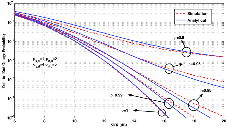
Figure 1: Outage probability for OR-DF mode over imperfect Log-normal fading channels for different $\rho$.

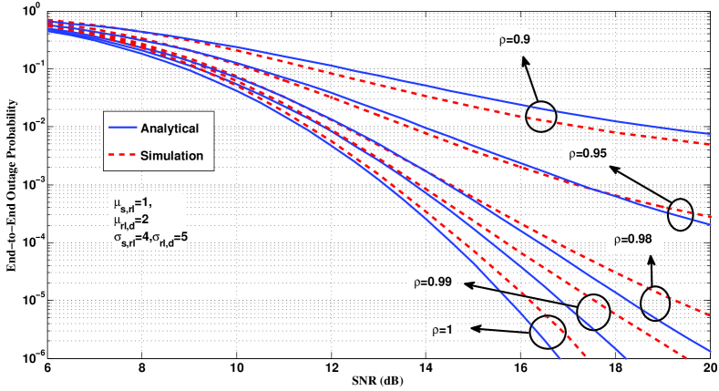
Figure 2: Outage probability for OR-AF mode over imperfect Log-normal fading channels for different $\rho$.

Using (23), the outage probability of the OR-AF relaying over imperfect non-identical fading channels can be expressed as

$$P_{out}=\prod_{l=1}^{L}Q(\frac{\mu_{\hat{\gamma}_{d,r_{l}}^{eff}}-10\log_{10}\hat{\gamma}}{\sigma_{\hat{\gamma}_{d,r_{l}}^{eff}}}).$$ (35)

V Numerical Results

In order to justify our analytical results, we provide some monte-carlo simulations in this section. In all simulations, unless it mentioned otherwise, we have three relays ($L=3$), $\gamma_{th}=3$, and $\rho_{s,r_{l}}=\rho_{r_{l},d}$. Log-normal fading channel parameters and the correlation coefficient between the exact and estimated channel, $\rho$, are given in each figure. We can calculate the variance of the each channel ($\sigma_{h}^{2}$) using [22]

$$\sigma_{h}^{2}=\mu_{X}^{2}({10^{\sigma_{X}^{2}{\textstyle{{\ln 10}\over{100}}}}}-1),$$ (36)

where, $\mu_{X}$ and $\sigma_{X}^{2}$ are the Log-normal fading parameters.

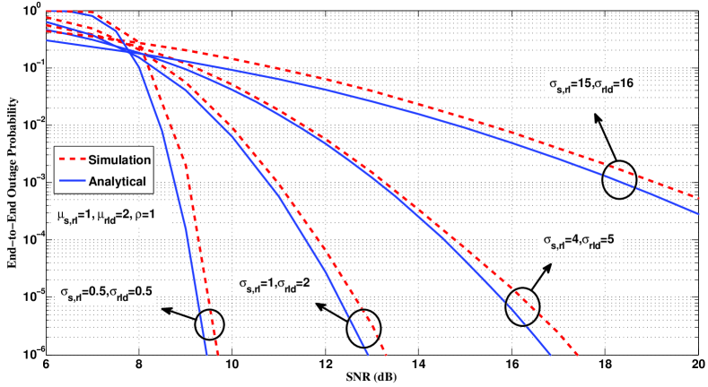
Figure 3: Comparing the accuracy of the analytical outage probability derived for OR-AF using Wilkinson method with the monte-carlo simulation.

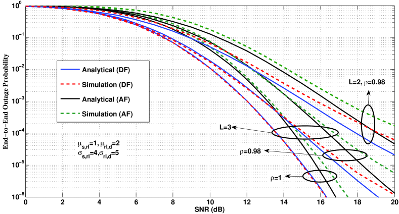
Figure 4: Comparison between analytical and simulated outage probability of OR-DF and OR-AF scheme with imperfect CSI with different number of relays. ($L=2$, $3$)

Fig.1 and Fig. 2 depict the effect of channel estimation error on OR-DF and OR-AF protocol over Log-normal fading channel, respectively. $\sigma_{l_{1}}$, $\mu_{l,1}$, $\sigma_{l_{2}}$, $\mu_{l_{2}}$ are the parameters of the first and second hop, respectively. Following conclusions are drawn from Figs. 1 and 2 :

1. As the $\rho$ decreases, or equivalently, the estimation error increases, the performance become worse.

2. As $\rho$ decreases the distance between the simulation and analytical result increases.

3. Depending on $\rho$, in a specific SNR, the performance of the system saturates, that is by increasing SNR, we do not get improvement in the system performance.

The second conclusion, is the outcome of the approximation that was mentioned in section III. However, simulations show that approximating the estimated channel as a Log-normal R.V is acceptable. We observe that for $\rho\simeq 1$, the analytical result is acceptable for good range of SNRs.

Fig. 3 investigate the accuracy of Wilkinson method with different variances for OR-AF system. As it is shown in [24], we see that the higher the variance, the higher the difference between the parameters of the approximated pdf according to Wilkinson method and the pdf according to simulation.

As it has been mentioned in [4], we can see that in Fig. 4 the DF outperforms the AF protocol in low SNRs; however, they become close to each other in high SNRs. We can also notice that the number of cooperating relays has a strong impact on the performance enhancement, that is the achieved diversity order is related to relay number, $L$.

VI Conclusion

In this paper, end-to-end outage probability of a wireless communication system using best-worse and best-harmonic mean selection Over Imperfect Non-identical Log-normal Fading Channels has been investigated. Channel estimation error has been considered as a Gaussian random variable. Since the distribution of estimated channels are not Log-normal either as would be in the case of the Rayleigh fading channels, simulation results do not exactly follow the analytical results. However, this difference is negligible for a wide variety of situations. Harmonic mean of two Log-normal R.Vs in presence of channel estimation errors was also derived.

VII Acknowledgements

This work has been supported by Iran Telecommunication Research Center (ITRC).

References

• [1] J. Laneman, D. Tse, and G. Wornell, “Distributed space-time-coded protocols for exploiting cooperative diversity in wireless networks,” IEEE Trans. Inform. Theory, vol. 49, no. 10, pp. 2415–2425, Sept. 2003.
• [2] ——, “Cooperative diversity in wireless networks: Efficient protocols and outage behavior,” IEEE Trans. Inform. Theory, vol. 50, no. 12, pp. 3062–3080, Dec. 2004.
• [3] M. O. Hasna and M. S. Alouini, “Outage probability of multihop transmission over Nakagami-m fading channels,” IEEE Trans. Commun., vol. 7, no. 5, pp. 216– 218, May 2003.
• [4] ——, “End-to-end performance of transmission systems with relays over Rayleigh-fading channels,” IEEE Trans. Wireless Commun., vol. 2, no. 6, pp. 1126 – 1131, Nov. 2003.
• [5] ——, “Harmonic mean and end-to-end performance of transmission systems with relays,” IEEE Trans. Commun., vol. 52, no. 1, pp. 130–135, Jan. 2004.
• [6] P. Anghel and M. Kaveh, “Exact symbol error probability of a cooperative network in a Rayleigh-fading environment,” IEEE Trans. Wireless Commun., vol. 3, no. 5, pp. 1416– 1421, Sept. 2004.
• [7] A. Ribeiro, X. Cai, and G. B. Giannakis, “Symbol error probabilities for general cooperative links,” IEEE Trans. Wireless Commun., vol. 4, no. 3, pp. 1264– 1273, May 2005.
• [8] S. S. Ikki and M. H. Ahmed, “Performance of cooperative diversity using equal gain combining (EGC) over Nakagami-m fading channels,” IEEE Trans. Wireless Commun., vol. 8, no. 2, pp. 557–562, Feb. 2009.
• [9] A. Bletsas, A. Khisti, D. Reed, and A. Lippman, “A simple cooperative diversity method based on network path selection,” IEEE J. Select. Areas Commun., vol. 24, no. 3, pp. 659– 672, March 2006.
• [10] A. Bletsas, A. G. Dimitriou, and J. N. Sahalos, “Interference-limited opportunistic relaying with reactive sensing,” IEEE Trans. Wireless Commun., vol. 9, no. 1, pp. 14–20, Jan. 2010.
• [11] T. Duong, V. N. Q. Bao, and H. j. Zepernick, “On the performance of selection decode-and-forward relay networks over Nakagami-m fading channels,” IEEE Commun. Lett., vol. 13, no. 3, pp. 172 –174, Mar. 2009.
• [12] Y. Zhao, R. Adve, and T. J. Lim, “Symbol error rate of selection amplify-and-forward relay systems,” IEEE Commun. Lett., vol. 10, no. 11, pp. 757 –759, Nov. 2006.
• [13] I. Kostic, “Analytical approach to performance analysis for channel subject to shadowing and fading,” IEE Proceedings Communications, vol. 152, no. 6, pp. 821 – 827, Dec. 2005.
• [14] M. Safari and M. Uysal, “Cooperative diversity over Log-normal fading channels: performance analysis and optimization,” IEEE Trans. Wireless Commun., vol. 7, no. 5, pp. 1963–1972, May 2008.
• [15] M. Renzo, F. Graziosi, and F. Santucci, “A comprehensive framework for performance analysis of cooperative multi-hop wireless systems over Log-normal fading channels,” IEEE Trans. Commun., vol. 58, no. 2, pp. 531–544, Feb. 2010.
• [16] M. Di Renzo, F. Graziosi, and F. Santucci, “Performance of cooperative multi-hop wireless systems over Log-normal fading channels,” in Proc. IEEE Global Telecommunications Conference ( GLOBECOM ’08), Nov. 2008, pp. 1–6.
• [17] M.-S. Alouini and M. K. Simon, “Dual diversity over correlated Log-normal fading channels,” IEEE Trans. Commun., vol. 50, no. 12, pp. 1946 – 1959, Dec. 2002.
• [18] C. S. Patel, G. L, Stüber, and T. G. Pratt, “Statistical properties of amplify and forward relay fading channels,” IEEE Trans. Veh. Technol., vol. 55, no. 1, pp. 1–9, Jan. 2006.
• [19] S. Han, S. Ahn, E. Oh, and D. Hong;, “Effect of channel-estimation error on ber performance in cooperative transmission,” IEEE Trans. Veh. Technol., vol. 58, no. 4, pp. 2083 –2088, May 2009.
• [20] M. Seyfi, S. Muhaidat, and J. Liang, “Amplify-and-forward selection cooperation with channel estimation error,” in IEEE Global Telecommunications Conference (GLOBECOM 2010), Miami, Florida, USA, Dec. 2010, pp. 1–6.
• [21] D. Gu and C. Leung, “Performance analysis of transmit diversity scheme with imperfect channel estimation,” Electronics Letters, vol. 39, no. 4, pp. 402 – 403, feb 2003.
• [22] A. Papoulis, Probability, Random variables, and Stochastic Processes.   New York: McGraw-Hill, 1991.
• [23] M. Simon and M. Alouini, Digital Communications Over Fading Channels.   Wiley & Sons, INC., Publication, 2005.
• [24] S. C. Schwartz and Y. S. Yeh, “On the distribution function and moments of power sums with Log-normal components,” Bell Syst. Tech. J., vol. 61, no. 7, pp. 1441–1462, Sept. 1982.