Secrecy Energy Efficiency Optimization for MISO and SISO Communication Networks

Abstract

Energy-efficiency, high data rates and secure communications are essential requirements of the future wireless networks. In this paper, optimizing the secrecy energy efficiency is considered. The optimal beamformer is designed for a MISO system with and without considering the minimum required secrecy rate. Further, the optimal power control in a SISO system is carried out using an efficient iterative method, and this is followed by analyzing the trade-off between the secrecy energy efficiency and the secrecy rate for both MISO and SISO systems.

I Introduction

Due to the presence of several wireless devices in a specific environment, the transmitted information may be exposed to unintended receivers. Using cryptography in higher layers, a secure transmission can be initiated. Nevertheless, it is probable that a unintended device, which maybe also be a part of the legitimate network, breaks the encryption [1]. Fortunately, physical layer security techniques can further improve the security by perfectly securing a transmission rate using the “secrecy rate” concept introduced in [2]. While security is a concern, power consumption is also another important issue in wireless communications since some wireless devices rely on limited battery power.

There are a wealth of research works in the literature which investigate the energy efficiency in wireless networks such as [3, 4] and the references therein. Recently, some research has been done to jointly optimize the secrecy rate and the power consumption. Sum secrecy rate and power are jointly optimized in [5] to attain a minimum quality of service (QoS). In [6], switched beamforming is used to maximize the secrecy outage probability over the consumed power ratio. Powers consumption for a fixed secrecy rate is minimized in [7] for an amplify-and-forward (AF) relay network. The secrecy outage probability over the consumed power is maximized subject to power limit for a large scale AF relay network in [8]. The optimal beamformer for a wiretap channel with multiple-antenna nodes is designed in [9] to maximize secrecy rate over power ratio.

Here, we consider a multiple-input single-output (MISO) and a single-input single-output (SISO) scenario while a single-antenna unintended receiver, which is part of the network, is listening. The secrecy rate over the power ratio, named “secrecy energy efficiency” and denoted by $\zeta$, is maximized with and without considering the minimum required secrecy spectral efficiency, denoted by $\eta_{0}$, at the destination. For comparison, we derive the optimal beamformer when zero-forcing (ZF) technique is used to null the signal at the eavesdropper with considering the minimum required secrecy spectral efficiency. Note that the ZF can only be used for the MISO scenario. Furthermore, the trade-off between $\zeta$ and secrecy spectral efficiency, denoted by $\eta$, is studied.

The following issues distinct our work from the most related research. In [9], first-order Taylor series expansion and Hadamard inequality are used to approximate the optimal beamfromer for a MIMO system. However, the exact beamformer for the MISO system is derived in this paper. Furthermore, the innermost layer of algorithm in [9] is based on the singular value decomposition, and is not applicable to SISO and MISO systems. In this paper, apart from the MISO system exact beamformer design, exact optimal power allocation for the SISO system is also derived.

The remainder of the paper is organized as follows. In Section II, we introduce the system model. The optimization problems are defined and solved in Sections III and IV. In Section V, the trade-off between secrecy energy efficiency and secrecy spectral efficiency is studied. Numerical results are presented in Section VI, and the conclusion is drawn in Section VII.

II Signal and System Model

Consider a wireless communication network comprised of a transmitter denoted by $T$, a receiver denoted by $R$, and an unintended user denoted by $E$. Note that to obtain the secrecy rate, the legitimate user needs to be aware of the instantaneous channel to the eavesdropper. This knowledge for the most general case with a passive eavesdropper is not practical. In this work, the unintended user is assumed to be part of the network. Therefore, the transmitter $T$ is able to receive the training sequence from $E$, in order to estimate its channel. The signal model and the secrecy rates are derived in the following parts.

II-A MISO System

Here, we assume that the transmitter employs multiple-antennas. The received signals at $R$ and $E$ are then as follows

$${y_{R}}={\bf{h}}_{T,R}^{T}{\bf{w}}x+{n_{R}},$$ (1)

$${y_{E}}={\bf{h}}_{T,E}^{T}{\bf{w}}x+{n_{E}},$$ (2)

where $x$ is the transmitted message, $\bf{w}$ is a vector containing beamforming gains, ${\bf{h}}_{T,R}$ and ${\bf{h}}_{T,E}$ are the transmitter’s channel gains toward the receiver and eavesdropper, respectively. The additive white Gaussian noise at the receiver and eavesdropper are shown by $n_{R}$ and $n_{E}$, respectively. The random variables $x$, $n_{R}$, and $n_{E}$ are complex circularly symmetric (c.c.s.) and independent and identically Gaussian distributed (i.i.d.) with $x\sim\mathcal{CN}(0,1)$, $n_{R}\sim\mathcal{CN}(0,\sigma_{{n_{R}}}^{2})$, and $n_{E}\sim\mathcal{CN}(0,\sigma_{{n_{E}}}^{2})$, respectively, where $\mathcal{CN}$ denotes the complex normal random variable. The noise powers, $\sigma_{{n_{R}}}^{2}$ and $\sigma_{{n_{E}}}^{2}$, are equal to $KT_{i}B$ where $K$ is the boltzman constant, $T_{i}$ is the temperature at the corresponding receiver with $i\in\{R,E\}$, and $B$ is the transmission bandwidth. Using (1) and (2) and the result in [10], the secrecy spectral efficiency (or rate in bps/Hz) denoted by $\eta$ is obtained by

$${\eta_{MISO}}={\left[{\log\left({\frac{{1+a}}{{1+b}}}\right)}\right]^{+}},$$ (3)

where $a=\frac{{{{\left|{{\bf{h}}_{T,R}^{T}{\bf{w}}}\right|}^{2}}}}{{\sigma_{{n_{R}}}^{2}}}$, $b=\frac{{{{\left|{{\bf{h}}_{T,E}^{T}{\bf{w}}}\right|}^{2}}}}{{\sigma_{{n_{E}}}^{2}}}$, and ${\left[x\right]^{+}}$ denotes $\max\left({x,0}\right)$. In this paper, all the logarithms are in base two. Further, the operator ${\left[\cdot\right]^{+}}$ is dropped throughout the paper for the sake of simplicity.

II-B SISO System

When one antenna is employed at the transmitter, using the result in [11], the secrecy spectral efficiency, $\eta$, is calculated as

$${\eta_{SISO}}={\left[{\log\left({\frac{{1+a^{\prime}}}{{1+b^{\prime}}}}\right)}\right]^{+}},$$ (4)

where $a^{\prime}=\frac{{P{{\left|{{h_{T,R}}}\right|}^{2}}}}{{\sigma_{{n_{R}}}^{2}}}$, $b^{\prime}=\frac{{P{{\left|{{h_{T,E}}}\right|}^{2}}}}{{\sigma_{{n_{E}}}^{2}}}$, $P$ is the transmission power by $T$, and ${h_{{T},{R}}}$ and ${h_{{T},{E}}}$ are the channel gains to the receiver and eavesdropper, respectively. The statistical characteristics of the message signal and the noise are the same as those in Section II-A.

III Problem Formulation: MISO System

In this section, we maximize $\zeta$ in a MISO system by obtaining the optimal beamformer for the cases with and without QoS constriant at the receiver.

III-A With QoS at the Receiver

The metric $\zeta$ is defined as $\eta$ multiplied by bandwidth over the total consumed power ratio as

$$\zeta=\frac{{B\eta}}{{{\left\|{\bf{w}}\right\|^{2}}+{P_{c}}}},$$ (5)

where $P_{c}$ is the circuit power consumption. We define our problem so as to maximize the secrecy energy efficiency subject to the peak power and QoS constraints as follows

$$\mathop{\max}\limits_{{\bf{w}}}\,\,\zeta\qquad\text{s.t.}\qquad{\left\|{\bf{w}}\right\|^{2}}\leq{P_{\max}},\,\,\eta>{\eta}_{0}.$$ (6)

To design the optimal beamformer, we rewrite (6) as

$$\mathop{\max}\limits_{\bf{w}}B\frac{{\log\left({\frac{{\sigma_{{n_{E}}}^{2}}}{{\sigma_{{n_{R}}}^{2}}}\frac{{\sigma_{{n_{R}}}^{2}+{{\bf{w}}^{H}}{\bf{h}}_{T,R}^{*}{\bf{h}}_{T,R}^{T}{\bf{w}}}}{{\sigma_{{n_{E}}}^{2}+{{\bf{w}}^{H}}{\bf{h}}_{T,E}^{*}{\bf{h}}_{T,E}^{T}{\bf{w}}}}}\right)}}{{{{\left\|{\bf{w}}\right\|}^{2}}+{P_{c}}}}$$

$$\,\,\text{s.t.}\qquad\left\|{\bf{w}}\right\|^{2}\leq{P_{\max}},\,\,{{\bf{w}}^{H}}{\bf{Cw}}\geq{2^{{\eta}_{0}}}-1,$$ (7)

where ${\bf{C}}=\frac{{{\bf{h}}_{T,R}^{*}{\bf{h}}_{T,R}^{T}}}{{\sigma_{{n_{R}}}^{2}}}-\frac{{{\bf{h}}_{T,E}^{*}{\bf{h}}_{T,E}^{T}}}{{\sigma_{{n_{E}}}^{2}}}{2^{{\eta}_{0}}}$. Using an auxiliary variable as $t=\left\|{\bf{w}}\right\|^{2}$, (7) is reformulated as follows

$$\mathop{\max}\limits_{{\bf{w}},0<t\leq P_{\max}}{\rm{B}}\frac{{{{\log}}\left({\frac{{\sigma_{{n_{E}}}^{2}}}{{\sigma_{{n_{R}}}^{2}}}\frac{{{{\bf{w}}^{H}}{\bf{Aw}}}}{{{{\bf{w}}^{H}}{\bf{Bw}}}}}\right)}}{{t+{P_{c}}}}$$

$$\,\text{s.t.}\,\,{\left\|{\bf{w}}\right\|^{2}}=t,\,\,{{\bf{w}}^{H}}{\bf{Cw}}\geq{2^{{\eta}_{0}}}-1,$$ (8)

where ${\bf{A}}={\frac{{\sigma_{{n_{R}}}^{2}}}{t}\bf{I}+{\bf{h}}_{T,R}^{*}{\bf{h}}_{T,R}^{T}}$ and ${\bf{B}}={\frac{{\sigma_{{n_{E}}}^{2}}}{t}\bf{I}+{\bf{h}}_{T,E}^{*}{\bf{h}}_{T,E}^{T}}$. The constraint $\left\|{\bf{w}}\right\|^{2}\leq{P_{\max}}$ is omitted since the upper limit of the search on variable shall be $P_{\max}$, which satisfy this constraint. To make the last constraint convex, (8) is transformed to a semidefinite programming (SDP) optimization problem.

$$\mathop{\max}\limits_{{\bf{W}},0<t\leq P_{\max}}{\rm{B}}\frac{{{{\log}}\left({\frac{{\sigma_{{n_{E}}}^{2}}}{{\sigma_{{n_{R}}}^{2}}}\frac{{\text{tr}\left({{\bf{WA}}}\right)}}{{\text{tr}\left({{\bf{WB}}}\right)}}}\right)}}{{t+{P_{c}}}}$$

$$\,\text{s.t.}\,\,\,\text{tr}\left({\bf{W}}\right)=t,\,\text{tr}\left({{\bf{WC}}}\right)\geq{2^{{{\eta}_{0}}}}-1,\,\bf{W}\succeq 0,$$ (9)

where $\text{rank}(\bf{W})=1$ constraint is dropped to have a set of convex constraints. Similar to [12], matrix $\bf{V}$ and scalar $s$ are defined such that ${\bf{V}}=s{\bf{W}}$ and $\text{tr}\left({s{\bf{WB}}}\right)=1$. Accordingly, (9) is transformed into

$$\mathop{\max}\limits_{{\bf{V}},0<t\leq P_{\max},s}\frac{{\rm{B}}}{{t+{P_{c}}}}{\log}\left({\frac{{\sigma_{{n_{E}}}^{2}}}{{\sigma_{{n_{R}}}^{2}}}\text{tr}\left({{\bf{VA}}}\right)}\right)$$

$$\,\text{s.t.}\qquad\text{tr}\left({\bf{V}}\right)=st,\,\,\text{tr}\left({{\bf{VC}}}\right)\geq s\left({{2^{{{\eta}_{0}}}}-1}\right),$$

$$\qquad\,\,\,\,\,\,\,\,\text{tr}\left({{\bf{VB}}}\right)=1,{\bf{V}}\succeq 0,s\geq 0.$$ (10)

Finally, by considering the auxiliary variable $t$ to be fixed and dropping the $\log$ due to the monotonicity of logarithm function, (10) can be solved using SDP along with a one-dimensional search over the variable $t$ where $t\in(0,P_{\max}]$. Since the matrices $\bf{A}$, $\bf{B}$, and $\bf{C}$ in (10) are Hermitian positive semidefinite, Theorem 2.3 in [13] can used to derive an equivalent rank-one solution if the solution to (10) satisfies $\text{rank}({\bf{W}})\geq 3$.

In order to perform a comparison, we also design the optimal beamforming vector to maximize the secrecy energy efficiency when zero-forcing (ZF) strategy is used to null the received signal at the eavesdropper. Using (7), the ZF beamformer design problem can be defined as follows

$$\mathop{\max}\limits_{\bf{w}}B\frac{{\log\left({\frac{{\sigma_{{n_{R}}}^{2}+{{\bf{w}}^{H}}{\bf{h}}_{T,R}^{*}{\bf{h}}_{T,R}^{T}{\bf{w}}}}{{\sigma_{{n_{R}}}^{2}}}}\right)}}{{{{\left\|{\bf{w}}\right\|}^{2}}+{P_{c}}}}$$

$$\,\text{s.t.}\,\,\left\|{\bf{w}}\right\|^{2}\leq{P_{\max}},\,{{\bf{w}}^{H}}{\bf{Cw}}\geq{2^{{\eta}_{0}}}-1,\,{\bf{h}}_{T,E}^{T}{\bf{w}}=0.$$ (11)

Using $t={{\bf{w}}^{H}}{\bf{w}}$, we get

$$\mathop{\max}\limits_{\bf{w}}\frac{B}{{t+{P_{c}}}}\left({\log\left({{{\bf{w}}^{H}}{\bf{Aw}}}\right)-\log\sigma_{{n_{R}}}^{2}}\right)$$

$$\,\text{s.t.}\,\,{\left\|{\bf{w}}\right\|^{2}}=t,\,{{\bf{w}}^{H}}{\bf{Cw}}\geq{2^{{\eta}_{0}}}-1,\,{\bf{h}}_{T,E}^{T}{\bf{w}}=0,$$ (12)

which can be simplified into

$$\mathop{\max}\limits_{\bf{w}}{{{\bf{w}}^{H}}{\bf{Aw}}}$$

$$\,\text{s.t.}\,\,{\left\|{\bf{w}}\right\|^{2}}=t,\,{{\bf{w}}^{H}}{\bf{Cw}}\geq{2^{{\eta}_{0}}}-1,\,{\bf{h}}_{T,E}^{T}{\bf{w}}=0.$$ (13)

To make the third constraint convex, similar to (8), (13) can be transformed into a SDP optimization problem as

$$\mathop{\max}\limits_{\bf{W}}\,\,\,\,\text{tr}\left({{\bf{WA}}}\right)$$

$$\,\text{s.t.}\,\,\text{tr}\left({\bf{W}}\right)=t,\,\text{tr}\left({{\bf{WC}}}\right)\geq{2^{{\eta}_{0}}}-1,$$

$$\,\,\,\,\,\,\,\,\,\,\text{tr}\left({{\bf{WD}}}\right)=0,{\bf{W}}\succeq 0,$$ (14)

where ${\bf{D}}={\bf{h}}_{T,E}^{*}{\bf{h}}_{T,E}^{T}$ and the rank-one constraint on $\bf{W}$ is dropped to make the problem convex. Since the matrices $\bf{A}$, $\bf{C}$, and $\bf{D}$ in (14) are Hermitian positive semidefinite, Theorem 2.3 in [13] can used to derive an equivalent rank-one solution if the solution to (14) satisfies $\text{rank}({\bf{W}})\geq 3$.

If the solution to (14) is not rank-one, Theorem 2.3 in [13] can be employed to derive an equivalent rank-one solution. Problem (14) can be solved using SDP along with a one-dimensional search over the variable $t$ where $t\in(0,P_{\max}]$.

III-B Without QoS at the Receiver

Using (8), the optimal beamformer design problem without considering the QoS is reduced to

$$\mathop{\max}\limits_{{\bf{w}},0<t\leq P_{\max}}{\rm{B}}\frac{{{{\log}}\left({\frac{{\sigma_{{n_{E}}}^{2}}}{{\sigma_{{n_{R}}}^{2}}}\frac{{{{\bf{w}}^{H}}{\bf{Aw}}}}{{{{\bf{w}}^{H}}{\bf{Bw}}}}}\right)}}{{t+{P_{c}}}}\,\,\text{s.t.}\,\,{\left\|{\bf{w}}\right\|^{2}}=t.$$ (15)

For a fixed $t$, (15) can be written as

$$\mathop{\max}\limits_{\bf{w}}\frac{{\rm{B}}}{{t+{P_{c}}}}\frac{{\sigma_{{n_{E}}}^{2}}}{{\sigma_{{n_{R}}}^{2}}}\frac{{{{\bf{w}}^{H}}{\bf{Aw}}}}{{{{\bf{w}}^{H}}{\bf{Bw}}}},$$ (16)

where $t\in(0,{P_{\max}}]$. Due to the homogeneity of (15), the constraints on the bamforming vector can be satisfied and thus dropped. The optimal value and the optimal beamforming vector in (16) are easily derived using Rayleigh-Ritz [14] when (16) is in its standardized form as

$$\mathop{\max}\limits_{\bf{v}}\frac{{\rm{B}}}{{t+{P_{c}}}}\frac{{\sigma_{{n_{E}}}^{2}}}{{\sigma_{{n_{R}}}^{2}}}\frac{{{{\bf{v}}^{H}}{\bf{Dv}}}}{{{{\bf{v}}^{H}}{\bf{v}}}},$$ (17)

where ${\bf{v}}={{\bf{C}}^{H}}{\bf{w}}$, $\bf{D}={{\bf{C}}^{-1}}{\bf{A}}{{\bf{C}}^{-H}}$, and matrix $\bf{C}$ is the Cholesky decomposition of matrix ${\bf{B}}$ as ${\bf{B}}={\bf{C}}{{\bf{C}}^{H}}$. The optimal beamforming vector is derived as ${{\bf{w}}^{\star}}={{\bf{C}}^{-H}}{{\bf{v}}^{\star}}$ where $\bf{v}^{\star}$ is the eigenvector corresponding to ${{\lambda_{\max}}\left({{{\bf{C}}^{-1}}\bf{A}{{\bf{C}}^{-H}}}\right)}$. Finally, the optimal $\zeta$ is obtained in closed-form by

$$\zeta{{}^{\star}}=B\frac{{{{\log}}\left({\frac{{\sigma_{{n_{E}}}^{2}}}{{\sigma_{{n_{R}}}^{2}}}{\lambda_{\max}}\left({{{\bf{C}}^{-1}}{\bf{A}}{{\bf{C}}^{-{\bf{H}}}}}\right)}\right)}}{{t+{P_{c}}}}.$$ (18)

Employing a one-dimensional search over $t\in(0,{P_{\max}}]$ and using (18), the optimal value of (17) is found.

IV Problem Formulation: SISO System

In the SISO case, the beamformer design is reduced to scalar power control. Similar to (6), the optimization problem for SISO system is defined as

$$\mathop{\max}\limits_{P}\,\,\,\,B\frac{{\log\left({\frac{{\sigma_{{n_{E}}}^{2}}}{{\sigma_{{n_{R}}}^{2}}}\frac{{\sigma_{{n_{R}}}^{2}+P{{\left|{{h_{T,R}}}\right|}^{2}}}}{{\sigma_{{n_{E}}}^{2}+P{{\left|{{h_{T,E}}}\right|}^{2}}}}}\right)}}{{{P_{c}}+P}}\,\,\text{s.t.}\,\,P_{\min}\leq P\leq{P_{\max}},$$ (19)

where ${P_{\min}}=\frac{{{2^{{\eta_{0}}}}-1}}{\alpha}$ is obtained from the minimum QoS constraint, and it is assumed that $\alpha=\frac{{{{\left|{{h_{T,R}}}\right|}^{2}}}}{{\sigma_{{n_{R}}}^{2}}}-\frac{{{{\left|{{h_{T,E}}}\right|}^{2}}}}{{\sigma_{{n_{E}}}^{2}}}{2^{{{\eta}_{0}}}}>0$. The numerator in the objective of (19) is concave since the argument of the logarithm is concave for $P\geq 0$ and $\frac{{{{\left|{{h_{T,R}}}\right|}^{2}}}}{{\sigma_{{n_{R}}}^{2}}}>\frac{{{{\left|{{h_{T,E}}}\right|}^{2}}}}{{\sigma_{{n_{E}}}^{2}}}$, which are granted in our problem, and the denumerator is affine. Hence, (19) is categorized as a family member of fractional programming problems known as “concave fractional program” where a local optimum is a global one [15]. Here, we solve (19) using an iterative (parametric) algorithm named Dinkelbach [16]. For the sake of simplicity, we mention the values related to ${\left|{{h_{T,R}}}\right|^{2}}$ and ${\left|{{h_{T,E}}}\right|^{2}}$ by $a$ and $b$, respectively. According to [16], after dropping the constant $B$, (19) is written as

$$F\left(q\right)=\mathop{\max}\limits_{P\in S}\log\left({\frac{{\sigma_{{n_{E}}}^{2}}}{{\sigma_{{n_{R}}}^{2}}}\frac{{\sigma_{{n_{R}}}^{2}+Pa}}{{\sigma_{{n_{E}}}^{2}+Pb}}}\right)-q\left({{P_{c}}+P}\right),$$ (20)

$$q=\frac{{f\left(P\right)}}{{g\left(P\right)}},$$ (21)

where $f(P)$ and $g(P)$ are the numerator and denumerator of (19), respectively. Also, $S$ shows the feasible domain of $P$. To calculate the optimal $P$ for (20), denoted by $P^{\star}$, the derivative of $F(q)$ with respect to $P$ is calculated as follows

$$\frac{{\partial F}}{{\partial P}}= -abq\beta{P^{2}}+Pq\beta\left({-a\sigma_{{n_{E}}}^{2}-b\sigma_{{n_{R}}}^{2}}\right)$$

$$+a\sigma_{{n_{E}}}^{2}-q\beta\sigma_{{n_{R}}}^{2}\sigma_{{n_{E}}}^{2}-b\sigma_{{n_{R}}}^{2},$$ (22)

which is a quadratic equation with a closed-form solution as

$${P_{1,2}}=\frac{{q\left({a\sigma_{{n_{E}}}^{2}+b\sigma_{{n_{R}}}^{2}}\right)\pm\sqrt{\Delta}}}{{-2abq}},\,\,\beta=\text{Ln}2,$$

$$\Delta={q^{2}}{\left({a\sigma_{{n_{E}}}^{2}+b\sigma_{{n_{R}}}^{2}}\right)^{2}}+4abq\left({a\sigma_{{n_{E}}}^{2}-q\sigma_{{n_{R}}}^{2}\sigma_{{n_{E}}}^{2}-b\sigma_{{n_{R}}}^{2}}\right).$$ (23)

Since $P_{1}$ in (23) is always negative, ${P^{\star}}$ is derived as

$$P^{\star}=\left\{{\begin{array}[]{*{20}{c}}P_{2}&P_{2}\in S,\\ \mathop{\arg}\limits_{P}\mathop{\max}\limits_{P\in\left\{{{P_{\min}},{P_{\max}}}\right\}}\,\,F\left(q\right)&P_{2}\notin S,\end{array}}\right.$$ (26)

where ${P_{2}}=\frac{{q\left({a\sigma_{{n_{E}}}^{2}+b\sigma_{{n_{R}}}^{2}}\right)-\sqrt{\Delta}}}{{-2abq}}$. The procedure to solve (19) using Dinkelbach method is summarized in Algorithm 1.

Algorithm 1 Iterative approach to solve (19)

1:Initialize $n=0$;

2:Pick any $P_{n}\in S$;

3:Derive $q_{n}$ using (21);

4:Derive $P^{\star}_{n}$ using (26) and calculate $F(q_{n})$ using (20);

5:if  $F(q_{n})\geq\delta$  then

6:     $n=n+1$;

7:     Go to 3;

8:end if

Using the closed-form solution of (20) given in (26), the following recursive relation is used to merge Steps 3 and 4 of Algorithm 1 as

$${P_{n+1}}=\frac{{\frac{{f\left({{P_{n}}}\right)}}{{g\left({{P_{n}}}\right)}}\left({a\sigma_{{n_{E}}}^{2}+b\sigma_{{n_{R}}}^{2}}\right)-\sqrt{{\Delta_{n}}}}}{{-2ab\frac{{f\left({{P_{n}}}\right)}}{{g\left({{P_{n}}}\right)}}}}.$$ (27)

It is proven in [16] that Algorithm 1 converges. In addition, since a local optimum for a concave fractional program is the global optimum, and (19) falls into this category, the solution found using Algorithm 1 is a global optimum.

V Trade-off between $\zeta$ and $\eta$

In this section, we study the trade-off between secrecy energy efficiency and secrecy spectral efficiency (i.e. $\zeta$ and $\eta$) for MISO and SISO systems.

V-A MISO System

To find the trade-off between $\zeta$ and $\eta$, we solve the optimal beamforming design problem to maximize $\zeta$ and $\eta$ separately for a specific power constraint, $P$. As a result, the pair $(\zeta,\eta)$ is available for different values of $P$. For $\zeta$, the optimization problem is as follows

$$\mathop{\max}\limits_{\bf{w}}{\mkern 1.0mu}{\mkern 1.0mu}B\frac{{{{\log}_{2}}\left({\frac{{\sigma_{{n_{E}}}^{2}}}{{\sigma_{{n_{R}}}^{2}}}\frac{{\sigma_{{n_{R}}}^{2}+{{\bf{w}}^{H}}{\bf{h}}_{T,R}^{*}{\bf{h}}_{T,R}^{T}{\bf{w}}}}{{\sigma_{{n_{E}}}^{2}+{{\bf{w}}^{H}}{\bf{h}}_{T,E}^{*}{\bf{h}}_{T,E}^{T}{\bf{w}}}}}\right)}}{{{P}+{P_{c}}}}\,\,\text{s.t.}\,\,\left\|{\bf{w}}\right\|^{2}=P.$$ (28)

Using the constraint in (28), we conclude that $\frac{{{{\bf{w}}^{H}}{\bf{w}}}}{{{P}}}=1$ which helps us homogenize (28) as

$$\mathop{\max}\limits_{\bf{w}}{\rm{B}}\frac{{{{\log}_{2}}\left({\frac{{\sigma_{{n_{E}}}^{2}}}{{\sigma_{{n_{R}}}^{2}}}\frac{{{{\bf{w}}^{H}}{\bf{Aw}}}}{{{{\bf{w}}^{H}}{\bf{Bw}}}}}\right)}}{{P+{P_{c}}}}\,\,\text{s.t.}\,\,\left\|{\bf{w}}\right\|^{2}=P,$$ (29)

where, ${\bf{A}}=\frac{{\sigma_{{n_{R}}}^{2}}}{P}{\bf{I}}+{\bf{h}}_{T,R}^{*}{\bf{h}}_{T,R}^{T}$ and ${\bf{B}}=\frac{{\sigma_{{n_{E}}}^{2}}}{P}{\bf{I}}+{\bf{h}}_{T,E}^{*}{\bf{h}}_{T,E}^{T}$. Similar to (15), the $\log$ and the power constraint can be dropped. Similar to the solution to (17), the optimal beamforming vector shall be ${{\bf{w}}^{\star}}={{\bf{C}}^{-H}}{{\bf{v}}^{\star}}$ where $\bf{v}^{\star}$ is the eigenvector corresponding to ${{\lambda_{\max}}\left({{{\bf{C}}^{-1}}\bf{A}{{\bf{C}}^{-H}}}\right)}$. The final closed-form solution for $\zeta{{}^{\star}}$ is

$$\zeta{{}^{\star}}=B\frac{{{{\log}}\left({\frac{{\sigma_{{n_{E}}}^{2}}}{{\sigma_{{n_{R}}}^{2}}}{\lambda_{\max}}\left({{{\bf{C}}^{-1}}{\bf{A}}{{\bf{C}}^{-{\bf{H}}}}}\right)}\right)}}{{P+{P_{c}}}}.$$ (30)

The optimal beamforming vector for $\eta{{}^{\star}}$ shall be the same as for $\zeta{{}^{\star}}$ and the optimal value of $\eta$ can be derived similar to the one for $\zeta$. Hence, the pair $(\zeta,\eta)$ is available.

V-B SISO System

By deriving $P$ with respect to $\eta$ using (4) as $P=\frac{{\sigma_{{n_{R}}}^{2}\sigma_{{n_{E}}}^{2}\left({{2^{\eta}}-1}\right)}}{{\sigma_{{n_{E}}}^{2}a-\sigma_{{n_{R}}}^{2}b{2^{\eta}}}}$, the relation between $\zeta$ and $\eta$ is calculated using (5) as follows

$$\zeta=\frac{{B\eta\left({\sigma_{{n_{E}}}^{2}a-\sigma_{{n_{R}}}^{2}b{2^{\eta}}}\right)}}{{\sigma_{{n_{R}}}^{2}\sigma_{{n_{E}}}^{2}\left({{2^{\eta}}-1}\right)+{P_{c}}\left({\sigma_{{n_{E}}}^{2}a-\sigma_{{n_{R}}}^{2}b{2^{\eta}}}\right)}}.$$ (31)

By solving $\frac{{d\zeta}}{{d\eta}}=0$ using numerical methods, $\eta$ corresponding to the optimal $\zeta$ can be derived.

VI Simulation Results

In this section, we present numerical examples to investigate the secrecy energy efficiency and its trade-off with the secrecy spectral efficiency. The simulations’ parameters are as follows. Distance from the transmitter to receiver and eavesdropper, $d$, is considered to be $2$ km, Quasi-static block fading channel model as $\mathcal{CN}(0,1)$, path loss is $128.1+37.6\log_{10}d$ dB [17], bandwidth is $20$ MHz, $P_{c}=5$, $P_{\max}=50$, receiver noise temperature is $298$ K, tolerance error for Dinkelbach algorithm is $\delta=10^{-3}$, and $N$ is the number of antennas. If the secrecy rate is negative, it is considered to be zero. For the figures presenting the average graphs, enough amount of channels are generated and the average of the resultant metrics are considered.

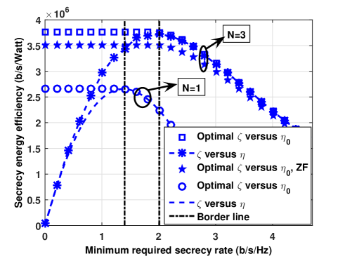
Figure 1: Optimal $\zeta$ versus $\eta_{0}$ and $\zeta$ versus $\eta$ graphs.

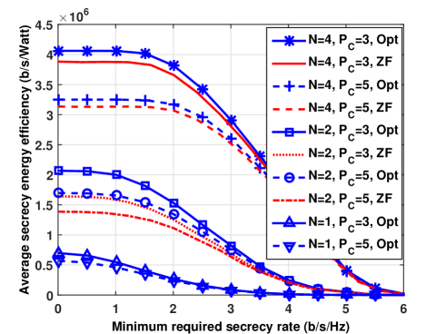
Figure 2: Average $\zeta$ versus ${\eta}_{0}$ for different $N$ and $P_{c}$.

In the first simulation scenario, the secrecy energy efficiency and secrecy spectral efficiency trade-off is studied. Optimal $\zeta$ versus the minimum required $\eta$ graphs as well as the graphs related to the trade-off between $\zeta$ and $\eta$ are presented in Fig. 1 using a single channel realization. Two different regions are defined in Fig. 1 using a border line. The border line defines the optimal operating point in terms of $\zeta$. In the left-hand side region, increasing $\eta$ also increases $\zeta$. Hence, to get a higher $\zeta$, the secrecy rate can be increased, which is desirable. However, the mechanism between $\zeta$ and $\eta$ changes in the right-hand side of Fig. 1. After the optimal point of $\zeta$, increasing $\eta$ demands more power which is higher than the optimal power value for $\zeta$. Therefore, as $\eta$ increases, $\zeta$ falls below the optimal value which is opposite to the procedure in the left-hand side, and the trade-off is clear. Also, it is observed that ZF results in a lower secrecy energy efficiency. Nevertheless, as the minimum required secrecy rate increases, the performance of the ZF approaches the primary scheme, i.e., optimal beamformer design.

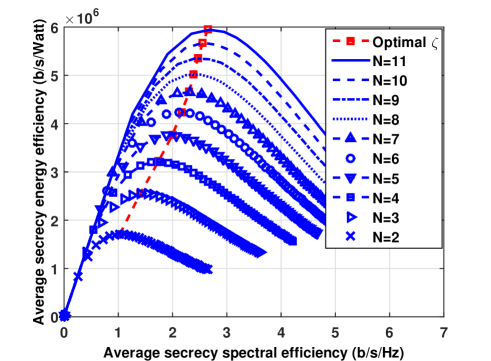
Figure 3: $\zeta$ and $\eta$ relation for different antennas.

For the second scenario, average $\zeta$ versus the minimum required $\eta$ is investigated for different numbers of antennas, and circuit powers. The related graphs are depicted in Fig. 2. As it is shown, increasing the number of antennas results in increasing the optimal value of $\zeta$ and makes it stable for a longer range of $\eta_{0}$. Further, we can see that decreasing $P_{c}$ leads to higher secrecy energy efficiency, and this is more significant for higher number of antennas. Similar to the result in Fig. 1, ZF scheme shows a sub-optimal performance. ZF’s performance gets closer to the optimal scheme as the circuit power, $P_{c}$, increases. Interestingly, for fewer number of antennas, the gap between the performance of the ZF and the optimal scheme even gets larger. This is due to less degrees of freedom for the ZF beamformer design as the number of antennas decreases. To investigate the trade-off between $\zeta$ and $\eta$, the average $\left({\zeta,\eta}\right)$ pair for different number of antennas is presented in Fig. 3. It is observed that the optimal $\zeta$ grows as number of antennas are increased.

VII Conclusion

In this work, we studied the secrecy energy efficiency, $\zeta$, and its trade-off with the secrecy spectral efficiency, $\eta$, in MISO and SISO wiretap channels. Optimal beamformer was designed to maximize $\zeta$ for the cases with and without considering the minimum required $\eta$ (i.e., $\eta_{0}$) at the receiver in a power limited system. We saw that as $\eta_{0}$ increases, the performance of the optimal beamformer and the ZF beamformer designs gets closer. Furthermore, as the number of antennas decreases, the performance gap between the optimal and the ZF design increases. It was observed that there is a specific $\eta$ below which increasing $\eta$ leads to higher secrecy energy efficiency (i.e., $\zeta$), and above which the opposite trend occurs. Depending on the power value corresponding to the optimal $\zeta$, increasing $\eta$ can increase or decrease $\zeta$. In addition, it was shown that adding more antennas to the transmitter side increases $\zeta$ considerably and sustains the optimal $\zeta$ for a longer range of $\eta_{0}$.

References

• [1] N. Sklavos and X. Zhang, Wireless Security and Cryptography: Specifications and Implementations.   Taylor & Francis, 2007.
• [2] A. D. Wyner, “The wire-tap channel,” Bell Systems Technical Journal, vol. 54, no. 8, pp. 1355–1387, Jan. 1975.
• [3] S. Cui, A. Goldsmith, and A. Bahai, “Energy-efficiency of MIMO and cooperative MIMO techniques in sensor networks,” IEEE J. Sel. Areas Commun., vol. 22, no. 6, pp. 1089–1098, Aug. 2004.
• [4] E.-V. Belmega and S. Lasaulce, “Energy-efficient precoding for multiple-antenna terminals,” IEEE Trans. Signal Process., vol. 59, no. 1, pp. 329–340, Jan. 2011.
• [5] D. Ng, E. Lo, and R. Schober, “Energy-efficient resource allocation for secure OFDMA systems,” IEEE Trans. Veh. Technol., vol. 61, no. 6, pp. 2572–2585, Jul. 2012.
• [6] X. Chen and L. Lei, “Energy-efficient optimization for physical layer security in multi-antenna downlink networks with QoS guarantee,” IEEE Commun. Lett., vol. 17, no. 4, pp. 637–640, Apr. 2013.
• [7] L. Wang, X. Zhang, X. Ma, and M. Song, “Joint optimization for energy consumption and secrecy capacity in wireless cooperative networks,” in IEEE Wireless Communications and Networking Conference (WCNC), Shanghai, China, Apr. 2013, pp. 941–946.
• [8] J. Chen, X. Chen, T. Liu, and L. Lei, “Energy-efficient power allocation for secure communications in large-scale MIMO relaying systems,” in IEEE/CIC International Conference on Communications in China (ICCC), Shanghai, China, Oct. 2014, pp. 385–390.
• [9] H. Zhang, Y. Huang, S. Li, and L. Yang, “Energy-efficient precoder design for MIMO wiretap channels,” IEEE Commun. Lett., vol. 18, no. 9, pp. 1559–1562, Sep. 2014.
• [10] F. Oggier and B. Hassibi, “The MIMO wiretap channel,” in International Symposium on Communications, Control and Signal Processing (ISCCSP), Malta, Mar. 2008, pp. 213–218.
• [11] J. Barros and M. Rodrigues, “Secrecy capacity of wireless channels,” in IEEE International Symposium on Information Theory, Seattle, WA, Jul. 2006, pp. 356–360.
• [12] A. De Maio, Y. Huang, D. Palomar, S. Zhang, and A. Farina, “Fractional QCQP with applications in ML steering direction estimation for radar detection,” IEEE Trans. Signal Process., vol. 59, no. 1, pp. 172–185, Jan. 2011.
• [13] W. Ai, Y. Huang, and S. Zhang, “New results on hermitian matrix rank-one decomposition,” Mathematical Programming, vol. 128, no. 1-2, pp. 253–283, Jun. 2011.
• [14] R. Horn and C. Johnson, Matrix Analysis.   Cambridge University Press, 1990.
• [15] S. Schaible and T. Ibaraki, “Fractional programming,” European Journal of Operational Research, vol. 12, no. 4, pp. 325–338, Apr. 1983.
• [16] W. Dinkelbach, “On nonlinear fractional programming,” Management Science, vol. 13, no. 7, pp. 492–498, Mar. 1967.
• [17] 3GPP, “3rd generation partnership project, technical specification group radio access network, coordinated multi-point operation for lte physical layer aspects,” Technical report 36.819, 2011-2012. [Online]. Available: http://www.3gpp.org