The transition from the classical to the quantum regime in nonlinear Landau damping.

Abstract

Starting from the Wigner-Moyal equation coupled to Poisson’s equation, a simplified set of equations describing nonlinear Landau damping of Langmuir waves is derived. This system is studied numerically, with a particular focus on the transition from the classical to the quantum regime. In the quantum regime several new features are found. This includes a quantum modified bounce frequency, and the discovery that bounce-like amplitude oscillations can take place even in the absence of trapped particles. The implications of our results are discussed.

I Introduction

Numerous aspects of quantum plasmas have been investigated during the last decade, see e.g. manfredi2006 ; Haas-book ; Shukla-Eliasson-RMP . Basic features such as electron degeneracy and particle dispersive properties have been studied in some detail manfredi2006 ; Haas-book ; Shukla-Eliasson-RMP ; Bret-2007 ; Andreev-2011 ; Vladimirov-2013 ; Brodin-2013 ; Surface-q ; Hall-MHD-q Exchange effects Manfredi-DFT ; Zamanian-exchange , the magnetic dipole force and other contributions from the electron spin Zamanian-2010-NJP ; Lundin-2010 have also been examined, including relativistic effects Asenjo-2011 ; Mend-2011 . Systems of interest in this context include e.g. quantum wells Manfredi-quantum-well , laser-plama interaction on solid density targets glenzer-redmer , and astrophysical plasmas Astro . Works on quantum plasmas also have relevance for recent applications in plasmonics Atwater-Plasmonics and spintronics Spintronics .

In the present paper we will consider the influence of quantum effects on the nonlinear regime of Landau damping, based on the Wigner-Moyal equation Haas-book that accounts for particle dispersive effects. Previous works in this area SFR-1991 ; Daligault-2014 have deduced that quantum effects can suppress the nonlinear bounce oscillations of Langmuir waves and turn the evolution into basic linear damping. Moreover, quantum corrections to electron holes in phase space that may form as a result of wave-particle interaction have been calculated in Ref. Fedele-2004 , and the quasilinear theory of the Wigner-Poisson system has been studied in Ref. Haas-2008 . However, many of the details of nonlinear Landau damping have not been studied before in the quantum regime. Making analytical approximations applicable for a resonance in the tail of the distribution, we first simplify the Wigner-Moyal equation coupled to Poisson’s equation into a system that is more easy to solve numerically. This system is shown to fulfill an energy conservation law, and reduces to a previously studied system Brodin-1997 in the classical limit. A systematic study of the transition from classical to quantum behavior then reveals several new features. This include a quantum modification of the bounce frequency, a new condition for the quantum suppression of the nonlinear regime and the discovery that bounce-like oscillations can take place even in the absence of trapped particles.

Similar to most cases, the conditions needed for quantum effects to be important in our problem include a high plasma density and a modest plasma temperature. However, while the scaling with temperature and density is the same as usual manfredi2006 ; Shukla-Eliasson-RMP , the precise numerical values are to some extent relaxed compared to the standard expressions in case the resonance lies in the tail of the distribution. The general conclusion is that the properties of wave-particle interaction are more easily influenced by quantum effects than the ordinary fluid properties. A concrete example is provided in the final section, and the significance of our results are discussed.

II Basic equations and derivations

Our starting point is the Wigner-Moyal equation Haas-book , which reads

$$\frac{\partial f}{\partial t}+\mathbf{v}\cdot\nabla f-\frac{iq}{\hbar}\int\frac{d^{3}\mathbf{r}^{\prime}d^{3}\mathbf{v}^{\prime}m^{3}}{(2\pi\hbar)^{3}}e^{i\mathbf{r}^{\prime}\cdot(\mathbf{v-v}^{\prime})m/\hbar}\left[\Phi(\mathbf{r}+\mathbf{r}^{\prime}/2)-\Phi(\mathbf{r}-\mathbf{r}^{\prime}/2)\right]f(\mathbf{r,v}^{\prime},t)=0$$ (1)

Here $f$ is the Wigner-function, $\Phi$ is the electrostatic potential, $q$ (=$-e$) is the electron charge, $m$ is the electron mass and $h=2\pi\hbar$ is Planck’s constant. Eq. (1) is combined with Poisson’s equation

$$-\nabla^{2}\Phi=\frac{q}{\varepsilon_{0}}\int fd^{3}\mathbf{v}$$ (2)

to give us a closed set. Eq. (1) applies for electrostatic fields and do not account for the spin of the electrons or exchange effects. For generalizations to electromagnetic fields and spin effects, see e.g. Ref. Zamanian-2010-NJP and for generalizations to include exchange effects, see e.g. Zamanian-exchange . Here we focus on the problem of Langmuir waves in an unmagnetized plasma, in which case the omissions of electromagnetic effects and spin effects are trivially justified. Furthermore, we will consider the case of a moderate plasma density with $\hbar\omega_{p}\ll k_{B}T$. It is then safe to exclude exchange effects Zamanian-exchange . In fact, the condition $\hbar\omega_{p}\ll k_{B}T$ is often used also to disregard the particle dispersive quantum effects included in Eq. (1). Such a condition is indeed an appropriate one for neglecting e.g. the particle dispersive contribution to the real part of the Langmuir dispersion relation and for neglecting the quantum contribution of Eq. (1) in many other cases manfredi2006 ; Haas-book ; Shukla-Eliasson-RMP . However, as we will see below, the quantum contribution to wave particle interaction can be crucial even in the regime $\hbar\omega_{p}\ll k_{B}T$.  A useful starting point to see this is to rewrite (1) in the alternative way Mendonca-2001

$$\frac{\partial f}{\partial t}+\mathbf{v}\cdot\nabla-\frac{q}{m}\Phi\cdot\left[\frac{2m}{\hbar}\sin\left(\frac{\hbar}{2m}\frac{\overleftarrow{\partial}}{\partial\mathbf{r}}\cdot\frac{\overrightarrow{\partial}}{\partial\mathbf{v}}\right)f\right]=0.$$ (3)

Here the arrows on the operators indicate in which direction they are acting, and the sinus-operator is defined in terms of its Taylor-expansion. Let us first consider linear plane wave solutions $\propto\exp i(kz-\omega t)$, and estimate the relative importance of quantum corrections. Letting $f=f_{0}+\hat{f}_{1}\exp i(kz-\omega t)$ we can use the classical linear solution

$$\hat{f}_{1}=\frac{qk\hat{\Phi}}{m(\omega-k_{z}v_{z})}\frac{\partial f_{0}}{\partial v_{z}}$$ (4)

as a means to illustrative the importance of quantum corrections. Comparing the magnitude of the first order quantum correction in the Taylor expansion with that of the classical term, we note that in the bulk of the velocity distribution (i.e. for $v\sim v_{t}$) the quantum corrections are small provided $Q_{\mathrm{bulk}}\ll 1$, where

$$Q_{\mathrm{bulk}}=\frac{\hbar k}{mv_{t}}.$$ (5)

However, looking at velocities close to the wave-particle resonance we must let $\omega-k_{z}v_{z}$ be small, of the order $\ \omega-k_{z}v_{z}\sim\gamma_{L}$ where $\gamma_{L}$ is the linear damping rate. Close to the resonance the relative importance of the quantum terms are given by the parameter $Q_{\mathrm{res}}$, which is

$$Q_{\mathrm{res}}=\frac{\hbar k^{2}}{m\gamma_{L}}.$$ (6)

For a resonance in the tail of the distribution $\gamma_{L}/k\ll v_{t}$ in which case we may have $Q_{\mathrm{res}}\sim 1$ at the same time as $Q_{\mathrm{bulk}}$ $\ll 1$. This regime will be the focus in what follows. As a result it suffices to solve the Vlasov limit of Eq. (3) in most of velocity space, but close to the resonance we need to solve the full Wigner equation. A similar approach applies for the small amplitude approximations. Provided $qk\hat{\Phi}/m\omega v_{t}\ll 1$ we have $\left|\partial\hat{f}_{1}/\partial v_{z}\right|\ll\left|\partial f_{0}/\partial v_{z}\right|$ unless we are close to the resonance. We will assume $qk\hat{\Phi}/m\omega v_{t}\ll 1$ to hold, and thus for most of velocity space we can solve the linearized Vlasov relation. However, close to the resonance where we can have nonlinear wave-particle interaction we must solve the Wigner equation without making linear approximations.

For a resonance in the tail of the distribution the number of particles contributing to the nonlinear interaction are relatively few. As a result there will be only minor harmonic generation of the electric field. Consequently we will use the ansatz of a slowly time-varying plane wave $\Phi=\hat{\Phi}(t)\exp i(kz-\omega t)+\mathrm{c.c}.$ for the potential, where c.c. stands for complex conjugate In general the Wigner function will be a periodic function, that will be represented as

$$f=f_{0}(\mathbf{v})+\delta f_{0}(\mathbf{v,}t)+\left[\sum_{n=1}^{\infty}f_{n}(\mathbf{v,}t)\exp i[n(kz-\omega t)]+\mathrm{c.c}\right].$$

Next we divide the velocity space into the resonant region $[v_{z}-\delta v_{\mathrm{res}},v_{z}+\delta v_{\mathrm{res}}]$ and the non-resonant region containing the complementary part.  When evaluating the charge density in (2) we thus use $\int fd^{3}v=\int_{\mathrm{nr}}fd^{3}v+\int_{\mathrm{res}}fd^{3}v$ where the subscripts nr and res denotes the nonresonant and resonant regions, respectively. Since the linear Vlasov equation applies in the nonresonant region we can use

$$\int_{\mathrm{nr}}fd^{3}v = \int_{\mathrm{nr}}f_{1}(\mathbf{v},t)e^{i(kz-\omega t)}d^{3}v+\mathrm{c.c}=$$ (7)

$$= \frac{qk\hat{\Phi}(t)}{m}\int_{\mathrm{nr}}\frac{e^{i(kz-\omega t)}(\partial f_{0}/\partial v_{z})}{(\omega-k_{z}v_{z})}d^{3}v-\int_{\mathrm{nr}}\frac{e^{i(kz-\omega t)}(\partial f_{1}/\partial t)}{i(\omega-k_{z}v_{z})}d^{3}v+\mathrm{c.c.}$$

Noting that the second term on the right hand side of (7) is a small correction, proportional to the slowly varying amplitude, we can use the lowest order approximation (i.e. dropping time derivatives on the amplitude) to convert it to a term proportional to $\partial\hat{\Phi}(t)/\partial t$. Combining (7) with (2) we then deduce

$$\frac{\partial\hat{\Phi}(t)}{\partial t}=\frac{q}{\varepsilon_{0}k^{2}\partial D/\partial\omega}\int_{\mathrm{res}}f_{1}d^{3}v$$ (8)

where $D(\omega,k)=1+(q^{2}/km\varepsilon_{0})$ $\int_{\mathrm{nr}}(\partial f_{0}/\partial v_{z})d^{3}v/(\omega-k_{z}v_{z})$. Note that the dispersion function $D(\omega,k)$ has a component of arbitrariness in the definition, since it depend on the width of the resonant region $\delta v_{\mathrm{res}}$. Nevertheless in the derivation of (8) we have taken $D(\omega,k)=0$ to hold by definition (i.e. $\omega(k)$ is defined by this relation), and in case a possible frequency shift occurs due to this, it is included in the time-dependence of $\hat{\Phi}\,$. It should be stressed that although a large number, of harmonics $f_{n}(\mathbf{v,}t)$ might be needed to solve for the Wigner function in the resonant region, it is only the first harmonic $f_{1}$ that contributes in (8).

Next we need to solve for the Wigner function in the resonant region. We restrict ourselves to a Maxwellian background distribution $F_{0}(\mathbf{v})$, and introduce the 1D-Wigner function

$$g=G_{0}(v_{z})+g_{0}(v_{z}\mathbf{,}t)+\left[\sum_{n=1}^{\infty}g_{n}(v_{z}\mathbf{,}t)\exp i[n(kz-\omega t)]+\mathrm{c.c}\right]$$ (9)

where $F_{0}(\mathbf{v})=G_{0}(v_{z})\exp[(-v_{x}^{2}-v_{y}^{2})/v_{t}^{2}]$ and $f_{n}(\mathbf{v},t)=g_{n}(v_{z},t)\exp[(-v_{x}^{2}-v_{y}^{2})/v_{t}^{2}]$. This ansatz is then substituted into (3). Since the gradient operator becomes $\pm ik\mathbf{\hat{z}}$ (as the spatial dependence of the potential is $\exp(\pm ikz)$) a useful formula is

$$\frac{2m}{\hbar}\sin\left(\pm\frac{i\hbar k}{2m}\frac{\partial}{\partial v_{z}}\right)g_{n}(v_{z},t)=\frac{\pm im\left[g_{n}(v_{z}+\hbar k/2m)-g_{n}(v_{z}-h\hbar/2m)\right]}{\hbar}.$$ (10)

With the help of this formula, and subsituting the ansatz (9) into (3), the following set of coupled equations are deduced

$$\frac{\partial g_{1}}{\partial t}-i\delta\omega(v_{z})g_{1} = \frac{q}{\hbar}\hat{\Phi}[G_{0}(v_{z}+\hbar k/2m)-G_{0}(v_{z}-\hbar k/2m)+g_{0}(v_{z}+\hbar k/2m)-g_{0}(v_{z}-\hbar k/2m)]$$ (11)

$$+\hat{\Phi}^{\ast}[g_{2}(v_{z}+\hbar k/2m)-g_{2}(v_{z}-\hbar k/2m)]$$

$$\frac{\partial g_{n}}{\partial t}-in\delta\omega(v_{z})g_{n} = \frac{q}{\hbar}\hat{\Phi}[g_{n-1}^{\ast}(v_{z}+\hbar k/2m)-g_{n-1}^{\ast}(v_{z}-\hbar k/2m)]+\hat{\Phi}^{\ast}[g_{n+1}(v_{z}+\hbar k/2m)-g_{n+1}(v_{z}-\hbar k/2m)]$$ (12)

and

$$\frac{\partial g_{0}}{\partial t}=\frac{q}{\hbar}\hat{\Phi}[g_{1}^{\ast}(v_{z}+\hbar k/2m)-g_{1}^{\ast}(v_{z}-\hbar k/2m)]+\hat{\Phi}^{\ast}[g_{1}(v_{z}+\hbar k/2m)-g_{1}(v_{z}-\hbar k/2m)]$$ (13)

where $\delta\omega(v_{z})=\omega-kv_{z}$ and the star denotes complex conjugate. Using $\int_{\mathrm{res}}f_{1}d^{3}v=\pi v_{t}^{2}\int_{\mathrm{res}}g_{1}dv_{z}$ in (8) we see that Eqs. (11)-(13) and (8) constitute a closed set. The equations agree with those studied by Ref. Brodin-1997 in the classical limit $\hbar\rightarrow 0$, provided the collisional frequency is put to zero in that work. It is clear that the quantum features are encoded in the velocity shift $\hbar k/2m$.  An important thing to note is that we can use $G_{0}(v_{z}+\hbar k/2m)-G_{0}(v_{z}-\hbar k/2m)\approx[\partial G_{0}(v_{z})/\partial v_{z}]\hbar k/m$ for $\hbar\omega/mv_{t}^{2}\ll 1$, whereas similar approximations are not applicable for the perturbed Wigner function, as the quantities $g_{n}$ varies on a much shorter scale length.

Before we can proceed we must put constraints on the parameter $\delta v_{\mathrm{res}}$. For the resonant region to cover a sufficient amount of resonant particles in the linear regime we need the condition $\delta v_{\mathrm{res}}\gg\gamma_{L}/k$. Moreover, to cover particles that are closed to be trapped in the potential well with a sufficiently large margin we need $\delta v_{\mathrm{res}}\gg\omega_{B}/k$, where $\omega_{B}=(qk^{2}\Phi/m)^{1/2}$ is the bounce frequency of trapped particles (with this choice the the resonant region is at least an order of magnitude larger than the region of trapped particles). Finally, to cover the quantum effects properly we need $\delta v_{\mathrm{res}}\gg\hbar k/2m$. At the same time the calculation scheme is based on the resonance region being much smaller than the thermal velocity, and hence we need $\delta v_{\mathrm{res}}\ll v_{t}$. If we sharpen this condition slightly and limit ourselves to $\delta v_{\mathrm{res}}\ll kv_{t}^{2}/\omega$ we may take $[\partial G_{0}(v_{z})/\partial v_{z}]$ as constant in the resonance region ($=[\partial G_{0}(v_{z})/\partial v_{z}]_{\omega/k}$), which simplify some of the technical aspects. For a resonance that lies in the tail of the distribution we can have $kv_{t}/\gamma_{L}\gtrapprox 100$, in which case it is easy to fulfill all conditions simultaneously, unless the nonlinearity or the quantum effects are extremely strong. Importantly, the numerical solutions presented below are not dependent on the precise choice of $\delta v_{\mathrm{res}}$, as long as the above conditions are fulfilled.

Next we introduce normalized variables. Choosing normalized time as $\gamma_{L}t$, normalized velocity as $kv_{z}/\gamma_{L}$, normalized potential as $qk^{2}\Phi/\gamma_{L}^{2}m$ and normalized harmonics of the Wigner function as

$$\frac{kg_{n}}{\gamma_{L}[\partial G_{0}(v_{z})/\partial v_{z}]_{\omega/k}}$$

the coupled equations become

$$\frac{\partial\hat{\Phi}(t)}{\partial t}=\frac{1}{\pi}\int_{\mathrm{res}}g_{1}dv$$ (14)

$$\frac{\partial g_{1}}{\partial t}+ivg_{1} = \hat{\Phi}\left[1+\frac{g_{0}(v+\delta v_{q})-g_{0}(v-\delta v_{q})}{2\delta v_{q}}\right]+\hat{\Phi}^{\ast}\left[\frac{g_{2}(v+\delta v_{q})-g_{2}(v-\delta v_{q})}{2\delta v_{q}}\right]$$ (15)

$$\frac{\partial g_{n}}{\partial t}+invg_{n} = \hat{\Phi}\left[\frac{g_{n-1}^{\ast}(v+\delta v_{q})-g_{n-1}^{\ast}(v-\delta v_{q})}{2\delta v_{q}}\right]+\hat{\Phi}^{\ast}\left[\frac{g_{n+1}(v+\delta v_{q})-g_{n+1}(v-\delta v_{q})}{2\delta v_{q}}\right]$$ (16)

and

$$\frac{\partial g_{0}}{\partial t}=\hat{\Phi}\left[\frac{g_{1}^{\ast}(v+\delta v_{q})-g_{1}^{\ast}(v-\delta v_{q})}{2\delta v_{q}}\right]+\hat{\Phi}^{\ast}\left[\frac{g_{1}(v+\delta v_{q})-g_{1}(v-\delta v_{q})}{2\delta v_{q}}\right]$$ (17)

where $n\geq 2$ in Eq. (16) and the quantum velocity shift is $\delta v_{q}=hk^{2}/2m\gamma_{L}$. We have omitted indices denoting normalized variables for notational convenience. Provided the conditions for the resonance region presented above is fulfilled, we may neglect perturbations at the boundary, i.e. use the approximation $g_{n}(\pm\delta v_{\mathrm{res}})\approx 0$ where $n=0,1,2...$.This property holds in the vicinity of the boundary (where the vicinity means a velocity of the order $\delta v_{q}$), which means that

$$\int_{\mathrm{res}}g_{0}(v+\delta v_{q})g_{1}^{\ast}(v)dv\approx\int_{\mathrm{res}}g_{0}(v)g_{1}^{\ast}(v-dv_{q})dv.$$ (18)

When $\delta v_{\mathrm{res}}$ is chosen large enough such that Eq. (18) is fulfilled, as well as similar types of approximations involving $g_{n}$, the system (14)-(17) posses an energy conservation law

$$\frac{\partial W_{\mathrm{tot}}}{\partial t}=\frac{\partial}{\partial t}\left[\left|\hat{\Phi}(t)\right|^{2}+\frac{1}{2}\int_{\mathrm{res}}g_{0}^{2}dv+\sum_{n=1}^{\infty}\int_{\mathrm{res}}\left|g_{n}\right|^{2}dv\right]=0$$ (19)

where $W_{\mathrm{tot}}$ is the total energy. The first term of Eq. (19) represents the wave energy (including the kinetic energy in the non-resonant region), whereas $\int_{\mathrm{res}}\left|g_{n}\right|^{2}dv$ represents the particle energy in the resonant region of each harmonic. Note that the zero:th harmonic get an extra factor $1/2$, which is related to $g_{0}$ being real. In the numerical calculation made in the next section Eq. (19) has been used as test of the numerical scheme and a confirmation that $\delta v_{\mathrm{res}}$ has been chosen large enough. In particular it should be stressed that the quantities $\int_{\mathrm{res}}\left|g_{n}\right|^{2}dv$ is not sensitive to the exact choice of $\delta v_{\mathrm{res}}$, since the integrand falls of rapidly away from the resonance. This can tested by varying the parameter $\delta v_{\mathrm{res}}$ in the numerical code. We find that the relative values of the wave energy and resonant energy changes around $0.001-0.002$ when the value of $\delta v_{\mathrm{res}}$ is changed a factor $1-3$ within the bounds of the strong inequalities.

An advantage with the above system (14)-(17) is that solving the equations numerically we can follow the evolution taking time-steps that are larger than the inverse plasma frequency, as the equations contain only the slow time-scales, as opposed to the original Wigner-Moyal equation (3). Moreover, we only need to solve the equations in a small part of the velocity space, close to the resonance, which also makes Eqs. (14)-(17) easier to solve numerically. Finally, the spatial dependence is solved for analytically in (14)-(17), which also simplifies the numerics.

III Remarks on the linear theory

Before we start with a numerical study, let us first make a few comments regarding the linear theory. As the equation stands, making a linearization of Eqs. (14)-(17) completely removes the quantity $\delta v_{q}$ which encodes the quantum properties. Eq. (15) can then be integrated according to

$$g_{1}=e^{-ivt}\int_{0}^{t}\hat{\Phi}(t^{\prime})e^{ivt^{\prime}}dt^{\prime}+e^{-ivt}g_{1}(t=0).$$ (20)

For certain initial conditions $g_{1}(t=0)$ the integrals in Eqs. (14) and (20) can be solved analytically (see e.g. Ref. Linear-ref for details), and for these cases we indeed have linear damping $\hat{\Phi}\propto e^{-t}$ which is written $e^{-\gamma_{L}t\text{ }}$in non-normalized units, where

$$\gamma_{L}=-\frac{\pi}{k}\frac{[\partial G_{0}(v_{z})/\partial v_{z}]_{\omega/k}}{\int_{\mathrm{nr}}\frac{\partial f_{0}/\partial v_{z}}{(\omega-k_{z}v_{z})^{2}}d^{3}v}.$$ (21)

The reason no effects due to the quantum treatment is seen here is the assumption of a modest quantum regime $kv_{t}^{2}/\omega\gg\delta v_{\mathrm{res}}\gg\hbar k/2m.$ These conditions apply for a resonance in the tail of the distribution, when the wavelength is not too short. Whenever these inequalities hold we can also use

$$G_{0}(v_{z}+\hbar k/2m)-G_{0}(v_{z}-\hbar k/2m)\simeq\frac{\hbar k}{m}\frac{\partial G_{0}}{\partial v_{z}}$$ (22)

which is the reason the finite difference is replaced by the classical expression containg a derivative in Eq. (21). Since $g_{0}$, $g_{1},g_{2}...$ varies on a much shorter scale length in velocity space as compared to $G_{0}$, we note that a similar approximation cannot be applied for these quantities. We stress that in a general scenario (e.g. for a beam-plasma system or for the regime $\hbar k^{2}/m\sim\omega$) the approximation (22) may give an incorrect description of linear Landau damping, but in our case the linear regime is classical to a good approximation. It shold also be noted that the evolution of $g_{1}$ exhibits phase mixing due to the factors $e^{-ivt}$ (see also Fig. 1 of the next section) whether or not the linear damping expression contains a finite difference or a derivative. Hence the quantum influence on the regime of linear Landau damping tend to be relatively modest also when the approximation (22) is avoided.

IV Numerical solutions

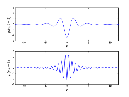
Figure 1: The real part of part of $g_{1}$ evaluated in the small amplitude regime for $t=2$ (upper panel) and $t=8$ (lower panel). The term $ivg_{1}$ of Eq. (15) leads to phase mixing, i.e. the development of increasingly small scales in velocity space. It should be noted that quantum effects does not counteract this behavior for small amplitudes.

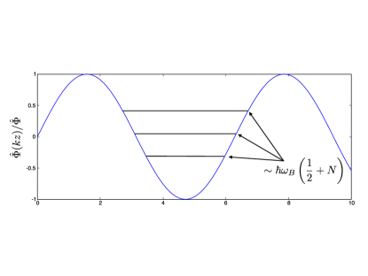
Figure 2: A qualitative illustration of the trapped particles. For a fixed wave amplitude particles trapped particles in the wave field have discrete energies, with an energy step of the order of $\hbar\omega_{B}$. When this becomes comparable to $q\hat{\Phi}$ only a few states are trapped, and quantum mechanical effects become important to describe the evolution.

The system (14)-(17) has been studied numerically using a staggered leapfrog finite differencing technique. Two classes of initial conditions have been used. In the first case $g_{1}(v,t=0)=\hat{\Phi}(t=0)/(iv+1)$ and $g_{0}(t=0)=g_{n}(t=0)$ $=0$ (for $n\geq 2$). This has the advantage that the Wigner function approaches the value outside the resonance reegion for $v\gg 1$. The other choice is to put also $g_{1}(v,t=0)=0$ such that the initial Wigner function is identically zero in the resonant region. It turns out that the evolution is almost completely independent of this difference in initial conditions, if the initial amplitude $\hat{\Phi}(t=0)$ is increased in the latter case such as to make the initial energy equal in the two cases. In what follows all numerical results will refer to the case with $g_{1}(v,t=0)=\hat{\Phi}(t=0)/(iv+1)$. Picking a small initial amplitude $\hat{\Phi}(t=0)\ll 1$ the system shows a damping $\hat{\Phi}\propto e^{-t}$ as expected due to the normalization of the time variable. As noted in the previous section the evolution is independent of the quantum parameter $\delta v_{q}$, which is related to the assumption $\hbar\omega/mv_{t}^{2}\ll 1$ that was made in the derivation. Fig. 1 compares the real part of $g_{1}$ for different times. The evolution shows the evolution towards smaller scale lengths in velocity space due to phase mixing. When nonlinearities come into play this  process plays part in increasing the relative importance of quantum effects in wave-particle interaction, as mathematically the system (14)-(17) differs from the classical limit once the scale length of $g_{n}$ in velocity space is smaller than $\delta v_{q}$. However, a more physical way to understand why quantum effects become important more easily in the nonlinear regime than in the linear regime is shown in Fig. 2. Here as a rough approximation we have described the discrete eigenstates of trapped particles as that of an harmonic oscillator where the eigenfrequency is the bounce frequency $\omega_{B}$. Naturally this is rather crude, as the electrostatic potential is only harmonic for the lowest energy states (if at all), and moreover the potential can vary dynamically to a smaller or larger degree depending on the parameters of the problem. Still the simple picture in Fig 2 is sufficient to identify one of the key parameters $R_{\mathrm{tr}}$, which is the ratio of the trapping potential over the energy quanta of trapped particles, $R_{\mathrm{tr}}=q\hat{\Phi}/\hbar\omega_{B}$. If the initial values have $R_{\mathrm{tr}}\gg 1$ the evolution of the wave amplitude $\hat{\Phi}(t)$ is classical to a good approximation. On the other hand, when $R_{\mathrm{tr}}$ decreases towards unity the discrete energy states of the trapped particles will modify the evolution significantly. In terms of our normalized variables we note that the quantum trapping parameter can be written as $R_{\mathrm{tr}}=q\hat{\Phi}/\hbar\omega_{B}=m\omega_{B}/\hbar k^{2}=\hat{\Phi}^{1/2}/\delta v_{q}$. For $R_{\mathrm{tr}}<1$ we will not have trapped particles. However, as we will see below the close coupling between the existence of trapped particles and nonlinear evolution that holds in the classical regime does not generally apply in the quantum regime.

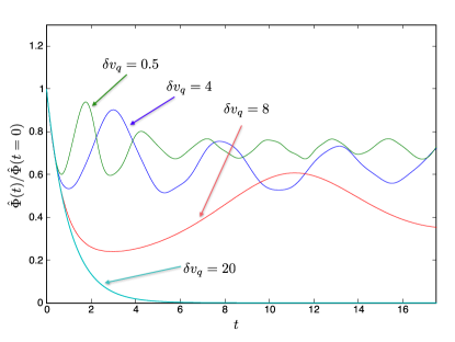
Figure 3: The evolution of $\hat{\Phi}(t)$ for initial amplitude $\hat{\Phi}(t=0)=4$ and $\delta v_{q}=0.5$, $4$, $8$ and $20$. The value $\delta v_{q}=0.5$ gives a classical evolution to a good approximation, whereas for $\delta v_{q}=20$ the nonlinearities are almost completely suppressed by the quantum effects.

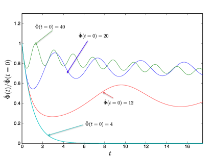
Figure 4: The evolution of $\hat{\Phi}(t)$ for $\delta v_{q}=20$. The inital amplitudes are $\hat{\Phi}(t=0)=4$, $12$, $20$ and $40$.

Next we investigate how the value of the quantum parameter $\delta v_{q}$ affects the evolution of $\hat{\Phi}(t)$ in the nonlinear regime. Keeping the normalized initial amplitude equal to $\hat{\Phi}(t=0)=4$ (which means that the (initial) bounce frequency is $\omega_{B}=2\gamma_{L}$), we follow the evolution up to $t=17.5$ for various values of $\delta v_{q}$. The result is shown in Fig. 3. For $\delta v_{q}\lesssim 1$ the evolution of the wave amplitude more or less coincides with the classical case. This means that an initial drop in amplitude is followed by oscillations with a frequency of the order of the bounce frequency $\omega_{B}$. As $\omega_{B}$ is not a constant, it is no surprise that these oscillations are slightly irregular. This result is in agreement with previous works on the classical case, see e.g. Brodin-1997 ; ONeil-1965 ; Manfredi-1997 . When the quantum parameter $\delta v_{q}$ is increased, more of the wave energy is converted to the particles (the initial amplitude drop is larger) and the period of the amplitude oscillations become longer. Eventually when $\delta v_{q}=20$ the initial amplitude drop is so large such that the evolution has become almost completely linear. Keeping $\delta v_{q}=20$ and instead varying the initial amplitude, the evolution $\hat{\Phi}(t)$ for various values of $\hat{\Phi}(t=0)$ is shown in Fig 4. The same qualitative features as in Fig 3 can be seen. That is the amplitude oscillation gets a lower frequency with decreasing $\hat{\Phi}(t=0)$, and the initial drop in wave amplitude is larger, until eventually for small enough initial amplitude the nonlinearities are suppressed and we obtain linear damping. A more quantitative analysis based on Figs 3 and 4 reveals that amplitude oscillations have a frequency $\omega_{\mathrm{amp}}\sim(\omega_{B}^{2}/(1+\delta v_{q})-\gamma_{L}^{2}/2)^{1/2}$ Classically $\delta v_{q}=hk^{2}/2m\gamma_{L}$ is small and $\omega_{\mathrm{amp}}\sim\omega_{B}$ for $\omega_{B}/\gamma_{L}\gg 1$. When the quantum velocity shift $\delta v_{q}$becomes comparable to the characteristic scale of $g_{1}$ the frequency of the amplitude oscillations decreases. Still the amplitude may oscillate nonlinearly even for large $\delta v_{q}$ and $R_{\mathrm{tr}}\ll 1$ (in the regime of no trapped particles). The transition to linear evolution occur when the expression for $\omega_{\mathrm{amp}}$ becomes begative, in which case the amplitude oscillation frequency decreases too fast for the nonlinear oscillations to get started.

Next we look closer on some of the details of the numerical results. As shown in Figs 3 and 4, the evolution of the wave amplitude changes rather smoothly with $\delta v_{q}$. However, the various harmonics of the Wigner function $g_{n}$ is more sensitive to the change in $\delta v_{q}$. The discrete structure involving momentum changes $\hbar k=2m\delta v_{q}$ can be seen directly in the Wigner function, perhaps most clearly in $g_{0}$. In a very rough sense there is a relation between the energy states displayed in Fig. 2 and the momentum structure shown in the upper panel of Fig. 5. As shown in Fig 5 where $g_{0}(v,t=10)$ is plotted in the classical and quantum mechanical regime, respectively, there is a very distinct difference between the quantum mechanical and classical regime. For the former case clear dips for $v\approx-2\delta v_{q}$ and $v\approx-\delta v_{q}$ can be seen, as well as peaks for $v\approx\delta v_{q}$ and $v\approx 2\delta v_{q}$. It should be noted, however, that a discrete structure in the momentum dependence can be seen even in the absence of trapped particles.

Another important aspect is the convergence in the sum over harmonics $g_{n}$, which is much faster in the quantum regime. A comparison of the classical and quantum regime is displayed in Fig. 6. We see that the relative amount of energy in the third harmonic $\int\left|g_{3}(t)\right|^{2}dv/W_{\mathrm{tot}}$ is changed dramatically when $\delta v_{q}$ is changed from $0.5$ to $4$. The convergence in the sum over the harmonics is determined by the trapping parameter $R_{\mathrm{tr}}$. In the classical and nonlinear regime with $R_{\mathrm{tr}}\gg 1$ we need to include harmonics up to $g_{10}$, or even more. Besides the value of $R_{\mathrm{tr}}$ the number of harmonics needed depends on the degree of the nonlinearity and how long the evolution is followed. In the quantum regime when $R_{\mathrm{tr}}>1$ including up to $g_{3}$ is typically more than enough to get convergence. This applies even when $\omega_{\mathrm{amp}}\gg\gamma_{L}$ and the evolution is strongly nonlinear. While the trapping parameter $R_{\mathrm{tr}}$ determines much of the properties of the Wigner function in the resonant region, it is the parameter $R_{\mathrm{nl}}=\omega_{B}^{2}/[\gamma_{L}^{2}(1+\delta v_{q})]=\hat{\Phi}/(1+\delta v_{q})$ that determines the degree of nonlinearity. In the nonlinear regime $R_{\mathrm{nl}}\gtrsim 1/2$  this parameter determines the frequency of the nonlinear amplitude oscillations, and we have $\omega_{\mathrm{amp}}^{2}=(R_{\mathrm{nl}}-1/2)\gamma_{L}^{2}$. For small $R_{\mathrm{nl}}$ (in practice $R_{\mathrm{nl}}<0.25$) the evolution is linear to a very good approximation. The reason why $R_{\mathrm{nl}}$ determines the nonlinearity can be understood roughly as follows: A key time-scale is the time-scale $t_{\mathrm{char}}$ for modifying the background distribution. Classically this time-scale is set by the inverse bounce-frequency, i.e. we have $t_{\mathrm{char}}^{2}\sim\omega_{B}^{-2}\propto$ $\hat{\Phi}^{-1}$. Mathematically this simply reflects the fact that the coupling to $g_{0}$ and the higher harmonics $g_{n}$ is linear in the wave amplitude, as seen in Eqs (15)-(17). When quantum effects enters the velocity derivative is replaced by a finite difference. Classically when the scale lengths in velocity space increases (cf Fig. 1) the magnitude of the nonlinear terms increases. However, the finite value of $\delta v_{q}$ prevents the continuous increase of the nonlinear coupling, as is seen from Eqs (15)-(17), and effectively the transition from classical to quantum regime correspond to a change $\hat{\Phi}\rightarrow\hat{\Phi}/(1+\delta v_{q})$. Physically this means that the characteristic time for acceleration of particles increases when the minimum velocity change comes in steps of $2\delta v_{q}$.  Noting that $\gamma_{L}^{2}t_{\mathrm{char}}^{2}>1$ for the nonlinear modifications of $g_{0}$ to occur faster than the linear damping explains the significance of the parameter $R_{\mathrm{nl}}$.

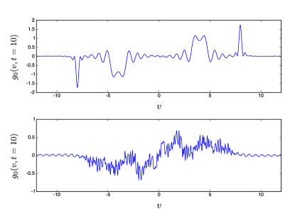
Figure 5: The profile of $g_{0}(v,t=10)$ shown for initial amplitude $\hat{\Phi}(t=0)=4$ for $\delta v_{q}=0.5$ (lower panel) and for $\delta v_{q}=4$ (upper panel). The discrete nature of the veloctiy dependence with peaks at discret values of $\delta v_{q}$ is clear in the quantum regime. There is also a relation to the discrete energy states of Fig. 2, since the discrete velocity structure disappears when there is a large number of trapped states, as seen in the lower panel. However, there is not a one-to-one correspondence between the energy states and the velocity structure. Specifically the discrete structure of the velocity dependence can be present in the strong quantum regime when the particle trapping is absent due to quantum effects.

The results reported here are similar in some respects to the findings of Ref. SFR-1991 and Ref. Daligault-2014 . In Ref. SFR-1991 the full Wigner equation was solved numerically. It was then found that the nonlinear regime of Landau damping was suppressed when $\hbar k/mv_{t}=8$. This is a rather extreme quantum regime, and our condition for suppressing the nonlinear regime (essentially $\omega_{\mathrm{amp}}^{2}$ being negative) which roughly gives $\hbar k^{2}/2m>\omega_{B}^{2}/\gamma_{L}$ is much easier to fulfill. The nmain reason for our relaxed quantum condition is that we have focused on a resonance in the tail of the distribution, where $\gamma_{L}\ll\omega$. In this case $\delta v_{q}$ become comparable to the velocity scale length close to the resonance long before $\delta v_{q}$ becomes comparable to the thermal (or Fermi) velocity. Thus we can investigate a regime where the wave-particle interaction is quantum mechanical, although the real part of the wave frequency is determined by the classical dispersion relation. By contrast, for a resonance in the bulk of the distribution, all quantum effects appear simultaneously. Next we compare our results with those of Ref. Daligault-2014 , that has studied the initial evolution of the wave particle interaction. We note that that the comparison of the quantum time-scales $t_{q}=2m/\hbar k^{2}$ with the classical bounce time $t_{B}$ $=2\pi/\omega_{B}$ made in Daligault-2014 is very similar to the discussion made above. In particular Ref. Daligault-2014 notes that the condition $t_{q}\ll$ $t_{B}$ implies the absence of trapped particles. However, since Ref. Daligault-2014 only studies the initial evolution, the conclusion that the nonlinear regime is suppressed for $t_{q}<t_{B}$ suggested in that work is not accurate. Using the notation of Daligault-2014 , rather the condition for suppressing the nonlinear regime is $t_{q}<t_{B}^{2}\gamma_{L}$, as explained above.

Much of the above features can be summarized in Fig. 7 that shows the different regimes of Landau damping plotted as a function of the nonlinearity parameter $\omega_{B}/\gamma_{L}$ and the quantum parameter $\hbar k^{2}/2m\gamma_{L}$. The interesting part of the diagram is the nonlinear quantum regime $\omega_{B}/\gamma_{L}\geq 1$ and $\hbar k^{2}/2m\gamma_{L}\geq 1$. It should be noted that the condition for quantum suppression of the nonlinear amplitude oscillations given by Ref. Daligault-2014 is the same condition that separates our region V from region VI (i.e. the condition that controls the existence of trapped particles). Interestingly, however, we find that the system can undergo nonlinear bounce-like oscillations even without trapped particles, and hence the region of quantum suppression (region IV) is determined by a distinct condition involving the quantum modified bounce frequency. It should be noted that the collisional influence can modify the different regimes to some extent. This will be discussed in some detail in the final section.

A feature of Fig. 4 not explained by the above discussion is the small but continuous decrease of wave energy seen for the highest amplitude in Fig. 4. Besides the amplitude oscillation there is a continuous decrease in $\hat{\Phi}(t)$ for initial condition $\hat{\Phi}(t=0)=40$ but not for $\hat{\Phi}(t=0)=20$. To understand this we must investigate how the energy of the particles in the resonance region is distributed among the harmonics. As described above the convergence is the sum over harmonics is fast for $R_{\mathrm{tr}}=\sqrt{\hat{\Phi}}/\delta v_{q}\ll 1$.   For the curves displayed in Fig 4 only the one with $\hat{\Phi}(t=0)=40$ has significant harmonic generation. For all the other curves the harmonics $g_{n}$ for $n\geq 2$ is effectively not excited, and the two terms $(1/2)\int_{\mathrm{res}}g_{0}^{2}dv+$ $\int_{\mathrm{res}}\left|g_{1}^{2}\right|dv$ accounts for more than $99\%$ of the particle energy. However, due to the rapid phase mixing of $g_{2}$ for large $\delta v_{q}$, this harmonics does not return the particle energy to wave energy, but instead the second harmonic acts as a leakage of energy, not taking part in bounce-like oscillations. This can be contrasted against the oscillatory evolution of the energy of the third harmonic for $\delta v_{q}=0.5$ which could be seen in Fig. 6. To a small extent the continuous loss of wave energy to higher harmonics can be observed also for $\hat{\Phi}(t=0)=20$, but to a much smaller degree. This is illustrated in Fig 8 , where the relative energy content in the second harmonic $\int_{\mathrm{res}}\left|g_{2}^{2}\right|dv/W_{\mathrm{tot}}$ is plotted for $\hat{\Phi}(t=0)=20$ and for $\hat{\Phi}(t=0)=40$. As can be seen, by a comparison with Fig. 4 the continuous increase of energy in the second harmonic accounts rather well for the overall downward trend in wave energy. A similar mechanism in principle exists also for lower values of $\delta v_{q}$. However here it is much less effective. The reason is twofold. Firstly, for lower $\delta v_{q}$ the peaks of $g_{2}$ and higher harmonics occurs for a smaller velocity, and phase mixing is less effective. Thus the energy of the higher harmonics can be returned back to lower harmonics more easily. Secondly,  for the same degree of nonlinearity (same value of $R_{\mathrm{nl}}$) the trapping parameter is larger for smaller $\delta v_{q}$. Hence a larger number of harmonics are excited for lower $\delta v_{q}$. This means that the highest harmonic excited takes a smaller proportion of the energy, in which case the leakage of energy is smaller. In practice, the details of the energy loss is likely to be determined by collisional effects, as very small scales in velocity space develops during the evolution Brodin-1997 .

Figure 6: Comparison of the relative energy in the third harmonic $\int\left|g_{3}(t)\right|^{2}dv/W_{\mathrm{tot}}$ for initial amplitude $\hat{\Phi}(t=0)=4$. The two curves are computed for $\delta v_{q}=0.5$ and for $\delta v_{q}=4$ respectively.

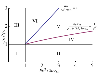
Figure 7: Summary of the different regimes of Landau damping for a resonance in the tail. Region I and II: Linear Landau damping. The quantum effects in region II does not change the value of the linear damping for a resonance in the tail Region III: Classical nonlinear regim with bounce oscillation of frequency $\sim\omega_{B}$. Region IV: Quantum suppression of nonlinear bounce-like oscillations. Region V: Nonlinear regime with bounce-like oscillations in the absence of trapped particles Region VI: Region of trapped particles with quantum modified bounce oscillations. Note that the same expression $\sim\omega_{B}/(1+\hbar k^{2}/m\gamma_{L})^{1/2}$ for the quantum modified amplitude oscillations apply in both region V and VI

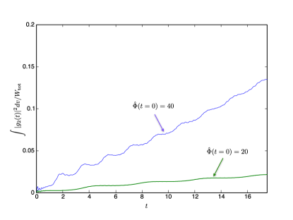
Figure 8: Comparison of the relative energy in the second harmonic $\int\left|g_{2}(t)\right|^{2}dv/W_{\mathrm{tot}}$ for $\delta v_{q}=20$. The two curves are computed for initial amplitude $\hat{\Phi}(t=0)=20$ and $\hat{\Phi}(t=0)=40$ respectively.

V Summary and Discussion

Usually particle dispersive effects as accounted for by the Wigner-Moyal equation are assumed to be significant when the thermal de Broglie length $\lambda_{\mathrm{dB}}=\hbar/mv_{\mathrm{t}}$, or its counterpart for a degenerate plasma, $\hbar/mv_{\mathrm{F}}$ (where $v_{\mathrm{F}}$ is the Fermi velocity),  becomes comparable to the Debye length $\lambda_{\mathrm{D}}=v_{\mathrm{t}}/\omega_{p}$ (or $v_{\mathrm{F}}/\omega_{p}$). The physics behind this condition is that the importance of collective effects require scale lengths not much shorter than the Debye length, and for the sinus-operator in Eq. (3) not to reduce to its classical limit we need $\hbar L_{\mathrm{char}}^{-1}/mv_{\mathrm{char}}$ $\sim 1$. If the characteristic spatial scale length $L_{\mathrm{char}}$ is assumed not to be smaller than $\lambda_{\mathrm{D}}$, and the velocity scale length $v_{\mathrm{char}}$ is of the order of $v_{\mathrm{t}}$ we get the condition $\hbar\omega_{p}/mv_{\mathrm{t}}^{2}\sim 1$ (or $\hbar\omega_{p}/mv_{\mathrm{F}}^{2}$ $\sim 1$ for a degenerate plasma) for quantum effects to be significant manfredi2006 ; Haas-book ; Shukla-Eliasson-RMP . This condition applies broadly to many situations, but does not hold for wave-particle interaction in general, as we have $v_{\mathrm{char}}\ll v_{\mathrm{t}}$ in case the resonance lies in the tail of the distribution. In the present paper, focusing on the case of Langmuir waves of a single wavelength, we have found that quantum effects become important in the nonlinear regime once $\hbar k^{2}/m\sim\omega_{B}$ in which case the trapped particle energies are quantized. Already when $\hbar k^{2}/m>\gamma_{L}$ nonlinear oscillations at the bounce frequency is slowed down in accordance with $\omega_{B}\rightarrow\omega_{B}/(1+\delta v_{q})^{1/2}$. While these oscillations are qualitatively similar to the well-known bounce oscillations ONeil-1965 , it should be noted that in the quantum regime such oscillations can occur even in the absence of trapped particles. Increasing the quantum parameter $\delta v_{q}$  even further, eventually the nonlinear oscillations are suppressed when $\omega_{B}/(1+\delta v_{q})^{1/2}<\gamma_{L}$ in which case usual linear damping takes place.

Since the phenomena of study evolves on a time scale slower than the plasma frequency, the above picture can be modified when the collisional influence is accounted for. Let us illustrate this by considering a concrete example. First we note that the long term evolution will always be affected by collisions. The characteristic time scale for collitions to be important $\tau_{\mathrm{c}}$ is given by $\min[\nu_{\mathrm{ei}}^{-1},\nu_{\mathrm{ee}}^{-1}]$.  To some extent we can assure that the phenomena of study occur on a faster scale by picking a relatively large amplitude and avoding a resonance too far out in the tail of the distribution. However, for a strongly coupled plasma this will not suffice, as $\nu_{\mathrm{ee}}$ approaches the plasma frequency rather than being a small parameter. Thus for our model to apply we must first of all consider a plasma that is weakly coupled. As an example we pick a plasma with a number density $n_{0}\simeq$ $10^{28}\mathrm{m}^{-3}$ and a temperature $T\simeq 10^{7}\mathrm{K}$ that correspond to a coupling parameter $\Gamma\simeq 0.01$. Such parameter values may result from laser-plasma experiments, see e.g. Ref. glenzer-redmer . Furthermore the temperature is well above the Fermi temperature, and we have a Debye length of the order $\lambda_{D}\simeq 10^{-9}\mathrm{m.}$ Adjusting the wavenumber we can chose the amount of resonant particles that determine the linear Landau damping rate and thereby pick he quantum parameter. In order to get $\delta v_{q}\simeq 4$ we can aim at $\gamma_{L}\simeq 10^{12}\mathrm{s}^{-1}$ which is obtained for a wave number $k\simeq 2\times 10^{8}\mathrm{m}^{-1}$. As $\delta v_{q}>1$ we are well in the quantum regime. We note, however, that although the plasma is weakly coupled, the time-scale for collisional damping is still shorter than the the linear damping time $\gamma_{L}^{-1}$. This is typically the case in the quantum regime, and hence the long-time evolution is generally much affected by collisions. However, most of our findings concern the nonlinear quantum behavior. As we will demonstrate below these findings are to a large extent still relevant even when collisions are taken into account. Firstly, the quantum modified bounce frequency $\omega_{B}$ $\rightarrow\omega_{B}/(1+\delta v_{q})^{1/2}$ can be experimentally verified after a few bounce oscillations. For example, if we pick $\hat{\Phi}\gtrsim 10\mathrm{V}$ the bounce oscillations take place on a much faster scale than collisional damping, in which case the quantum modification of the bounce frequency becomes detectable. Moreover, generally the prediction of a nonlinear regime in the absence of trapped particles (regime V in Fig. 7) can be verified after a few (quantum modified) bounce oscillations. Hence in an experimental situation we do not need to follow the evolution until collisional effects become important. The situation is somewhat different when it comes to the condition for quantum suppression of the nonlinear oscillations. It is possible to verify that previously given conditions are incorrect in agreement with our theory, as the presence of bounce oscillations at a faster scale than the linear damping rate will confirm this. However, the quantitative confirmation of our condition that separates regions IV and V in Fig 7 is likely not possible, as that would require us to study the system when the quantum modified bounce frequency is of the same order as the linear Landau damping rate. In this case we need to follow the evolution long enough such that collisions will modify the picture. Thus we conclude that most features of Fig 7 remains even when we account for collisional effects, but that there are restrictions arising from the collisional influence that makes the boundary between region IV and V uncertain.

While the study here has focused on Landau damping due to electrons, it should be noted that a similar process may take place for photons Mendonca-2001 ; Mendonca-2006 . Photon Landau damping can be relevant to Langmuir waves with relativistic phase velocities, in the presence of electromagnetic radiation, when resonant electrons are nearly absent. The wave nature of the photons provides the classical counterpart to the quantum electron states, and we can similarly identify a photon bounce frequency $\omega_{Bph}\sim\omega_{B}$. Photon trapping effects were experimentally observed by Murphy-2006 .

Acknowledgement This paper is dedicated to our good friend and colleague Professor Lennart Stenflo, celebrating his 75:th birthday.

References

- (1) G. Manfredi, Fields Inst. Commun. 46, 263 (2005).
- (2) F. Haas, Quantum Plasmas, A Hydrodynamics Approach (Springer, New York, 2011).
- (3) P. K. Shukla and B. Eliasson, Rev. Mod. Phys. 83, 885 (2011).
- (4) A. Bret, Phys. Plasmas 14, 084503 (2007).
- (5) P. A. Andreev, L. S. Kuzmenkov and M. I. Trukhanova, Phys. Rev. B, 84, 245401 (2011)
- (6) F. Sayed, S. V. Vladimirov, Yu. Tyshetskiy and O. Ishihara, Phys. Plasmas 20, 072116 (2013)
- (7) G. Brodin and M. Stefan, Phys. Rev. E 88, 023107 (2013).
- (8) M. Marklund, G. Brodin, L. Stenflo and C. S. Liu, Europhys. Lett, 84, 17006 (2008).
- (9) P. K. Shukla and L. Stenflo, J. Plasma Phys., 74, 575 (2008).
- (10) N. Crouseilles, P. -A Hervieux and G. Manfredi, Phys. Rev. B, 78, 155412 (2008).
- (11) J. Zamanian, M. Marklund and G. Brodin, Phys. Rev. E 88, 063105 (2013).
- (12) J. Zamanian, M. Marklund, G. Brodin, New J. Phys. 12, 043019 (2010).
- (13) J. Lundin and G. Brodin, Phys. Rev. E 82, 056407 (2010).
- (14) F. A. Asenjo, V. Munoz, J. A. Valdivia and S. M. Mahajan, Phys. Plasmas 18, 012107 (2011).
- (15) J.T. Mendonça, Phys. Plasmas 18, 062101 (2011).
- (16) G. Manfredi and P.-A. Hervieux, Appl. Phys. Lett. 91, 061108 (2007).
- (17) S. H. Glenzer and R. Redmer, Rev. Mod. Phys. 81, 1625 (2009).
- (18) A. K. Harding and D. Lai, Rep. Prog. Phys. 69, 2631 (2006).
- (19) H. A. Atwater, Sci. Am. 296, 56 (2007).
- (20) S. A. Wolf, D. Awschalom, R. A. Buhrman, et al., Science 294, 1488 (2001).
- (21) N. D. Suh, M. R. Feix and P. Bertrand, J. Compl. Phys. 94, 403 (1991).
- (22) J. Daligault, Phys. Plasmas, 21, 040701 (2014).
- (23) A. Luque, H. Schamel and R. Fedele, Phys. Lett. A, 324, 185 (2004).
- (24) F. Haas, B. Eliasson, P. K. Shukla, and G. Manfredi, Phys. Rev. E., 78, 056407 (2008).
- (25) G. Brodin, Phys. Rev. Lett. 78, 1263 (1997).
- (26) J. T. Mendonça, Theory of Photon Acceleration, (Bristol: Institute of Physics publishing, 2001).
- (27) G. Brodin, Am. J. Phys. 65, 66 (1997).
- (28) The staggered leapfrog method also works well when the finite differences in the right hand side is replaced by a velocity derivative, which corresponds to the classical limit. In the quantum regime Eqs. (15)-(17) just constitute a set of ordinary differential equations (although it is a large set, since the velocity resolution must be sufficient), and a fourth order Runge-Kutta method could also be applied.
- (29) T. M. O’Neil, Phys. Fluids 8, 2255 (1965).
- (30) G. Manfredi, Phys. Rev. Lett. 79, 2815 (1997).
- (31) J. T. Mendonça and A. Serbeto, Phys. Plasmas 13, 102109 (2006).
- (32) C. Murphy et al., Phys. Plasmas 13, 033108 (2006).