Phase of the fermion determinant in QED₃ using a gauge invariant lattice regularization

Abstract

We use canonical formalism to study the fermion determinant in different three dimensional abelian gauge field backgrounds that contain non-zero magnetic and electric flux in order to understand the non-perturbative contributions to the parity-odd and parity-even parts of the phase. We show that a certain phase associated with free fermion propagation along a closed path in a momentum torus is responsible for the parity anomaly in a background with non-zero electric flux. We consider perturbations around backgrounds with non-zero magnetic flux to understand the structure of the parity-breaking perturbative term at finite temperature and mass.

I Introduction

Three dimensional Euclidean abelian gauge theory coupled to a two component massless fermion by

$$D\!\!\!\!/\ ({\bf A})=\sigma_{k}\left(\partial_{k}+iA_{k}\right),$$ (1)

can induce a parity breaking mass term for the gauge field in the form of a Chern-Simons action Deser:1981wh ; Deser:1982vy ; Niemi:1983rq

$$S=\frac{i\kappa}{4\pi}\int d^{3}xA_{k}F_{k}\qquad\text{where}\qquad F_{k}=\epsilon_{kij}\partial_{i}A_{j}.$$ (2)

The mass term is gauge invariant in infinite volume provided the fields are assumed to vanish at infinity. This result has been shown in perturbation theory using the gauge invariant Pauli-Villars regularization Redlich:1983dv .

Theories with $2N$ flavors of massless fermions can have a real and positive determinant with proper pairing of fermions. Vacuum energy arguments show that the $O(2N)$ symmetry breaks down to $O(N)\times O(N)$ symmetry Vafa:1984xh and it has been shown that dynamical masses are generated for fermions that do not break parity Pisarski:1984dj in the large $N$ limit. Recent calculations along the same lines using Schwinger-Dyson equations Braun:2014wja attempt to identify the phase structure that separates one where dynamical masses are generated from others that do not. Numerical studies using staggered fermions Hands:2002dv ; Hands:2004bh ; Fiore:2005ps have been performed and condensates have been computed for theories that do not break parity, again with the aim of exploring the phase structure.

The gauge theory with one flavor of two component Dirac fermion can be regularized in a gauge invariant manner using the Wilson-Dirac operator So:1984nf ; So:1985wv ; Coste:1989wf

$$D_{w}({\bf U},M)=D\!\!\!\!/\ _{n}({\bf U})-B({\bf U})+M;\qquad D\!\!\!\!/\ _{n}^{\dagger}({\bf U})=-D\!\!\!\!/\ _{n}({\bf U});\qquad B^{\dagger}({\bf U})=B({\bf U}),$$ (3)

where ${\bf U}$ is the U(1) valued lattice link variable; $D\!\!\!\!/\ _{n}({\bf U})$ is the naïve lattice fermion operator; $B({\bf U})$ is the Wilson term that provides a mass of the order of cut-off for the doublers; and $0\leq M<1$ is the mass in lattice units for the fermion. Perturbation theory computations Coste:1989wf using Eq. (3) in infinite volume show that the coefficient of the induced Chern-Simons term in Eq. (2) is $\kappa=-1$ if $M>0$, and $\kappa=-\frac{1}{2}$ if one takes the massless limit after taking the continuum limit. For negative fermion masses, we would use

$$D_{w}({\bf U},-M)=-D^{\dagger}_{w}({\bf U},M)=D\!\!\!\!/\ _{n}({\bf U})+B({\bf U})-M\qquad\text{for}\qquad 0\leq M<1,$$ (4)

so that the induced parity breaking term as one approaches the massless limit from the positive and negative side are opposite in sign.

A theory with $2N$ flavors with $N$ flavors obeying Eq. (3) and the other $N$ flavors obeying Eq. (4) can be used for a numerical investigation of condensates that do not break parity. We can also consider theories with non-degenerate fermions and arbitrary number of flavors, and study the effect of parity breaking mass terms in the limit of large number of flavors.

Consider the continuum limit in a lattice simulation where we take the number of lattice points denoted by $L\to\infty$. The continuum limit needs to be taken keeping the physical spatial extent $l$, the fermion mass $m_{\rm phys}$ and the temperature $T$ constant as $L\to\infty$. In a lattice calculation, it is natural to instead consider the dimensionless temperature $t=lT$ and the dimensionless mass $m=lm_{\rm phys}$, measured in units of the spatial extent, to be the parameters of the theory and keep them constant as $L\to\infty$. Since we study fermions on fixed gauge field backgrounds, the coupling constant $g^{2}$ does not play a role in the present calculations. The induced gauge action in a fixed gauge field background will be gauge invariant and it is of interest to study this outside perturbation theory before embarking on a full lattice simulation. Of particular interest is the phase of fermion determinant which contains parity violating terms. Consider, for example Dunne:1998qy , a gauge field background that has a non-zero magnetic flux,

$$\int F_{3}dxdy=2\pi q_{3},$$ (5)

for integer $q_{3}$, along with a non-zero Polyakov loop, $e^{i\int A_{3}d\tau}=e^{i2\pi h_{3}}$. The associated Chern-Simons action is

$$S(h_{3},q_{3})=i\kappa\pi h_{3}q_{3},$$ (6)

and it has to remain invariant under the gauge transformation $h_{3}\to(h_{3}+1)$. This implies $\kappa$ has to be an even integer Pisarski:1986gr ; Henneaux:1986tt ; Hosotani:1989vz for this particular gauge field background in a regularization that preserves gauge invariance under such “large” gauge transformations Deser:1997nv ; Deser:1997gp ; Fosco:1997ei . This does not match with $\kappa=-1$ or $\kappa=-\frac{1}{2}$ obtained in Coste:1989wf . Effect of non-vanishing gauge fields at infinity on spontaneous and anomalous breaking of parity have also been addressed in Nissimov:1985wk . In addition to the parity violating contributions to the phase of the fermion determinant,

$$e^{i\Gamma(t,m,{\bf A})}=\lim_{L\to\infty}\frac{\det D_{w}(U,M)}{\left|\det D_{w}(U,M)\right|},$$ (7)

in the continuum limit, there are also parity preserving contributions of the form $e^{i\pi h(A)}$ where $h(A)$ are integers associated with zero crossings of the Wilson-Dirac operator AlvarezGaume:1984nf ; Forte:1986em ; Forte:1987kj .

As a precursor to studying the three dimensional theory, consider the regularized result using Wilson-Dirac fermions in one dimension in comparison to the results obtained in Dunne:1998qy ; Deser:1997nv ; Deser:1997gp ; Fosco:1997ei ; Kikukawa:1997qh . The Wilson-Dirac fermion operator in one dimension is

$$D_{w}(U,M)=-1+M+T,$$ (8)

where the translation operator $T$ is $(T\psi)(k)=U(k)\psi(k)$ in terms of the one dimensional link variable, $U(k)$. The only physical degree of freedom is the Polyakov loop,

$$W=\lim_{L\to\infty}\prod_{k=1}^{L}U(k)=e^{i2\pi h},$$ (9)

and the fermion determinant in the continuum, assuming $L$ to be even, is

$$\lim_{L\to\infty}\det D_{w}\left(U,\frac{m}{L}\right)=\begin{cases}e^{i2\pi h}-e^{-m}=\begin{cases}e^{i2\pi h}&m=\infty\cr 2\sin(\pi h)e^{i\pi h+i\frac{\pi}{2}}&m=0_{+}\end{cases}\cr e^{-i2\pi h}-e^{-m}=\begin{cases}2\sin(\pi h)e^{-i\pi h-i\frac{\pi}{2}}&m=0_{-}\cr e^{-i2\pi h}&m=-\infty.\end{cases}\end{cases}$$ (10)

The result matches with the one obtained in Deser:1997gp using zeta function regularization and has the main features discussed before. It is invariant under the “large” gauge transformation $h\to(h+1)$ for all values of $m$. The part of phase proportional to $h$ in the massless limit is half of its value in the infinite mass limit. As for the vacuum structure is concerned, the partition function for a two flavor theory with masses $m_{1}$ and $m_{2}$ is

$$Z(m_{1},m_{2})=\begin{cases}e^{-(m_{1}+m_{2})}&m_{1},m_{2}>0\cr e^{-(m_{1}-m_{2})}+1&m_{1}>0;\ \ m_{2}<0,\end{cases}$$ (11)

showing that the theory with $m_{1}>0$ and $m_{2}<0$ is preferred over $m_{1},m_{2}>0$.

The aim of this paper is to study the phase $\Gamma(t,m,{\bf A})$ in the continuum U(1) gauge field background on a three dimensional $l\times l\times\frac{1}{t}$ torus given by

$$A_{1}=\frac{2\pi q_{2}t}{l}\tau+\frac{2\pi h_{1}}{l}+A_{1}^{p};\qquad A_{2}=\frac{2\pi q_{3}}{l^{2}}x+\frac{2\pi h_{2}}{l}+A_{2}^{p};\qquad A_{3}=\frac{2\pi q_{1}t}{l}y+2\pi h_{3}t+A_{3}^{p},$$ (12)

where $q_{i}$ are integers and they denote non-zero flux in the $x$, $y$ and $\tau$-directions; $h_{i}\in[0,1]$ denotes torons generating non-trivial Polyakov loops; and $A_{i}^{p}$ are perturbative fields that obey periodic boundary conditions. The associated periodic boundary conditions on fermions are

$$\psi(l,y,\tau)=e^{-i\frac{2\pi q_{3}y}{l}}\psi(0,y,\tau);\qquad\psi(x,l,\tau)=e^{-i2\pi q_{1}\tau t}\psi(x,0,\tau);\qquad\psi(x,y,\frac{1}{t})=e^{-i\frac{2\pi q_{2}x}{l}}\psi(x,y,0).$$ (13)

We refer to $q_{3}$ as magnetic flux, and $q_{1}$ and $q_{2}$ as electric flux. The naming is not relevant if only one of the three is non-zero, but we also consider cases with $q_{1}\neq 0$, $q_{2}\neq 0$ and $q_{3}=0$ in this paper and extract some results without completely resorting to numerical means. In addition, we numerically study the most general case with non-zero flux in all three directions. The phase splits into a parity even and odd part

$$\Gamma=\Gamma_{\rm even}+\Gamma_{\rm odd},$$ (14)

with the parity even part being

$$\Gamma_{\rm even}=\pi(q_{1}+q_{2}+q_{3})+\pi(q_{1}q_{2}+q_{3}q_{1}+q_{2}q_{3}).$$ (15)

The first term can be absorbed by changing the boundary conditions of fermions but not both the first and second terms. In general, the parity odd part is complicated, but it has a simple form in the case of zero temperature when we consider a $\tau$-dependent perturbation on a static and spatially uniform magnetic field:

$$\Gamma_{\rm odd}=-2\pi h_{3}q_{3}-\int d\tau d\tau^{\prime}A_{1}^{p}(\tau)A_{2}^{p}(\tau^{\prime})G(\tau-\tau^{\prime}),$$ (16)

where the form factor $G(\tau)$ is an odd function of $\tau$ that depends on the fermion mass $m$ and spatial torons. Our formulation on the lattice enables us to study $G(\tau)$ without making prior assumptions concerning the local or non-local nature of the induced gauge action. We study how the form factor becomes local in the limit of $m\to\infty$ and $m\to 0$.

The organization of the paper is as follows. We describe lattice gauge fields on a torus in Section II. In Section III, we derive an expression for the Wilson-Dirac fermion determinant in the lattice axial gauge allowing for non-trivial Polyakov loops using the canonical formalism Hasenfratz:1991ax . In Section IV, we use the canonical formalism to study cases with uniform electric and magnetic fields, organized into subsections. Here, we explain the origin of the parity even phase in Eq. (15). First, we present a conventional way to understand the parity breaking when there is only a non-zero magnetic flux. The zero crossings of the eigenvalues of the two dimensional Dirac operator are responsible for the parity breaking terms and the formula for the fermion determinant using lattice regularization matches the one from zeta function regularization Deser:1997nv ; Deser:1997gp . We then consider the case where we have non-zero electric fluxes but zero magnetic flux. We show that the relevant quantity to obtain the parity even part of the phase is associated with the propagation of a free fermion with continuously changing momentum along a closed loop in the torus in momentum space in a direction defined by $(q_{2},-q_{1})$. Finally, we turn on perturbations over static magnetic field backgrounds. For this, we develop second order perturbation theory with in the canonical formalism in Section V and use it to study the parity odd part of the induced effective action. The results of the perturbative analysis and the numerical extraction of the form factor $G$ are presented in Section V.1 and Section V.2.

II Gauge field on a torus

We work on an $L^{2}\times\beta$ lattice for the sake of simplicity, which can be easily generalized to a spatially anisotropic lattice as well. We only consider lattices where both $L$ and $\beta$ are even; while the continuum physics is independent of this choice, it helps to simplify our calculations. The spatial volume of the lattice is defined as $V\equiv L^{2}$. The spatial lattice points are labelled by $\mathbf{x}=(x_{1},x_{2})$ with $1\leq x_{i}\leq L$, and the temporal lattice points by $k$ with $1\leq k\leq\beta$. The dimensionless temperature in the continuum limit is

$$t=\lim_{L\to\infty}\frac{L}{\beta}.$$ (17)

The continuum space and Euclidean time variables are

$$(x,y)=\lim_{L\to\infty}\left(\frac{x_{1}}{L},\frac{x_{2}}{L}\right)\qquad\text{and}\qquad\tau=\lim_{L\to\infty}\frac{k}{L},$$ (18)

with $x,y\in[0,1]$ and $\tau\in\left[0,\frac{1}{t}\right]$.

On this lattice, we introduce U$(1)$ gauge fields using the gauge-links $U_{\mu}(\mathbf{x},k)$. In this work, we fix the gauge such that the temporal gauge-links from $k=1$ to $k=\beta-1$ are set to identity. Non-trivial Polyakov loop variables in the $\tau$-direction are taken care of by the presence of $U_{3}(\mathbf{x},\beta)=U_{3}(\mathbf{x})$. This partial gauge fixing enables us to develop the canonical formalism in Section III. We still have a remnant time independent gauge symmetry, $g(\mathbf{x})$, under which

$$U_{i}(\mathbf{x},k)\to g^{\dagger}(\mathbf{x})U_{i}(\mathbf{x},k)g(\mathbf{x}+\hat{i})\quad\text{and}\quad U_{3}(\mathbf{x})\to g^{\dagger}(\mathbf{x})U_{3}(\mathbf{x})g(\mathbf{x}).$$ (19)

In this work, we consider only the gauge fields of the form in Eq. (12). An analogous Hodge-decomposition is strictly true for any gauge-fields in two dimensions. In three dimensions, one should consider these as specific background gauge fields used in order to probe the dependence of the fermion determinant on perturbative and non-perturbative aspects of the gauge-field. The gauge fields in Eq. (12) are periodic only up to a gauge transformation with non-trivial winding. Since we do not require smoothness of the link variables on the lattice, such gauge fields along with fermions, which satisfy the boundary conditions in Eq. (13), can be incorporated using gauge links and fermions that are strictly periodic. For our gauge choice, the lattice gauge field background corresponding to Eq. (12) is

$$U_{1}({\bf x},k) = \begin{cases}e^{i\frac{2\pi q_{2}}{L\beta}k}e^{i\frac{2\pi h_{1}}{L}+iA_{1}^{q}}&\text{if}\quad x_{1}<L\cr e^{i\frac{2\pi q_{2}}{L\beta}k-i\frac{2\pi q_{3}}{L}x_{2}}e^{i\frac{2\pi h_{1}}{L}+iA_{1}^{q}}&\text{if}\quad x_{1}=L,\cr\end{cases}$$ (20)

$$U_{2}({\bf x},k) = e^{i\frac{2\pi q_{3}}{L^{2}}x_{1}-i\frac{2\pi q_{1}}{\beta L}k}e^{i\frac{2\pi h_{2}}{L}+iA_{2}^{q}},$$ (21)

$$U_{3}({\bf x}) = e^{-i\frac{2\pi q_{2}}{L}x_{1}+i\frac{2\pi q_{1}}{L}x_{2}}e^{i2\pi h_{3}}.$$ (22)

The various background gauge fields we study in this paper are instances of the above equation.

III Canonical formalism

The partial gauge fixing defined in Section II naturally allows for the development of the Hamiltonian or the canonical formalism Hasenfratz:1991ax . Let $T_{i}(k)$ be the parallel transporters along spatial directions at a fixed Euclidean time, $k$:

$$\left[T_{j}(k)\psi\right](\mathbf{x})\equiv U_{j}(\mathbf{x},k)\psi(\mathbf{x}+\hat{j}),$$ (23)

and let $T_{3}$ defined as

$$\left[T_{3}\psi\right](\mathbf{x})\equiv U_{3}(\mathbf{x})\psi(\mathbf{x}),$$ (24)

be the parallel transporter that connects $k=\beta$ and $k=1$. In this gauge field background, the Wilson-Dirac fermion operator is

$$D^{kk^{\prime}}(M) = \left[-3+M+\frac{1}{2}\sum_{i=1}^{2}\left[\left(\sigma_{i}+1\right)T_{i}(k)-\left(\sigma_{i}-1\right)T_{i}^{\dagger}(k)\right]\right]\delta^{k^{\prime},k}$$ (26)

$$+\frac{1}{2}\begin{cases}\left[\left(\sigma_{3}+1\right)\delta^{k^{\prime},2}-\left(\sigma_{3}-1\right)T_{3}^{\dagger}\delta^{k^{\prime},\beta}\right]&\text{if}\quad k=1\cr\left[\left(\sigma_{3}+1\right)\delta^{k^{\prime},k+1}-\left(\sigma_{3}-1\right)\delta^{k^{\prime},k-1}\right]&\text{if}\quad 1<k<\beta\cr\left[\left(\sigma_{3}+1\right)T_{3}\delta^{k^{\prime},1}-\left(\sigma_{3}-1\right)\delta^{k^{\prime},\beta-1}\right]&\text{if}\quad k=\beta,\cr\end{cases}$$

where the second term takes care of the periodicity in the temporal direction. In this way, we have managed to write the Dirac operator using operators defined on two-dimensional time-slices. The Wilson mass $M$ is such that $|M|<1$. It is related to the physical mass $m$ in the units of box length as

$$m\equiv ML.$$ (27)

By using the following set of Pauli matrices,

$$\sigma_{1}=\begin{pmatrix}0&1\cr 1&0\cr\end{pmatrix};\ \ \ \ \sigma_{2}=\begin{pmatrix}0&-i\cr i&0\cr\end{pmatrix};\ \ \ \ \sigma_{3}=\begin{pmatrix}1&0\cr 0&-1\cr\end{pmatrix},$$ (28)

the Wilson-Dirac operator $D$ can be written in the matrix form as

$$D(M)=\begin{pmatrix}-B_{1}&C_{1}&1&0&\cdots&\cdots&0&0\cr-C_{1}^{\dagger}&-B_{1}&0&0&\cdots&\cdots&0&T_{3}^{\dagger}\cr 0&0&-B_{2}&C_{2}&\cdots&\cdots&0&0\cr 0&1&-C_{2}^{\dagger}&-B_{2}&\cdots&\cdots&0&0\cr\vdots&\vdots&\vdots&\ddots&\ddots&\ddots&\vdots&\vdots\cr\vdots&\vdots&\vdots&\vdots&\ddots&\ddots&\ddots&\vdots\cr T_{3}&0&0&0&\cdots&\cdots&-B_{\beta}&C_{\beta}\cr 0&0&0&0&\cdots&\cdots&-C_{\beta}^{\dagger}&-B_{\beta}\cr\end{pmatrix},$$ (29)

where

$$B_{k} \equiv 3-M-\frac{1}{2}\sum_{j=1}^{2}\left(T_{j}(k)+T^{\dagger}_{j}(k)\right),$$ (30)

$$C_{k} \equiv \frac{1}{2}\left(T_{1}(k)-T^{\dagger}_{1}(k)\right)-\frac{i}{2}\left(T_{2}(k)-T^{\dagger}_{2}(k)\right).$$ (31)

Note that $B_{k}$ is a positive definite operator for $|M|<1$. We closely follow Neuberger:1997bg in order to obtain an expression for the determinant of $D$. We first cyclically permute the columns to the left. This gives a matrix

$$D^{\prime}(M)=\begin{pmatrix}\alpha_{1}&0&0&\cdots&\cdots&0&\gamma_{1}Y\cr\gamma_{2}&\alpha_{2}&0&\cdots&\cdots&0&0\cr 0&\gamma_{3}&\alpha_{3}&\cdots&\cdots&0&0\cr\vdots&\vdots&\vdots&\ddots&\ddots&\vdots&\vdots\cr\vdots&\vdots&\vdots&\ddots&\ddots&\vdots&\vdots\cr 0&0&0&\cdots&\cdots&\alpha_{\beta-1}&0\cr 0&0&0&\cdots&\cdots&\gamma_{\beta}&\alpha_{\beta}X\cr\end{pmatrix},$$ (32)

where

$$\alpha_{k}\equiv\begin{pmatrix}C_{k}&1\cr-B_{k}&0\cr\end{pmatrix};\quad\gamma_{k}\equiv\begin{pmatrix}0&-B_{k}\cr 1&-C^{\dagger}_{k}\cr\end{pmatrix};\quad X\equiv\begin{pmatrix}1&0\cr 0&T_{3}\cr\end{pmatrix};\quad Y\equiv\begin{pmatrix}T_{3}^{\dagger}&0\cr 0&1\end{pmatrix}.$$ (33)

Using the formula for the determinant of the above matrix from Neuberger:1997bg , we arrive at

$$\det D(M)=\left[\prod_{j=1}^{\beta}\det\alpha_{j}\right]\det\left[X-\left(\prod_{k=\beta}^{1}{\cal T}_{k}\right)Y\right],$$ (34)

where the hermitean transfer matrix ${\cal T}_{k}$ associated with propagating the fermion across the $k$-th slice is

$${\cal T}_{k}\equiv-\alpha_{k}^{-1}\gamma_{k}=\begin{pmatrix}B^{-1}_{k}&-B^{-1}_{k}C^{\dagger}_{k}\cr-C_{k}B^{-1}_{k}&C_{k}B^{-1}_{k}C^{\dagger}_{k}+B_{k}\end{pmatrix}.$$ (35)

The final expression for the fermion determinant is

$$\det D(M)=\left(\prod_{j=1}^{\beta}\det B_{j}\right)\det T_{3}\det{\cal H}\qquad\text{where}\qquad{\cal H}\equiv{\mathbf{1}}-\left(\prod_{k=\beta}^{1}{\cal T}_{k}\right)T_{3}^{\dagger}.$$ (36)

This is the main formula that we use repeatedly in order to understand the phase of the determinant, $\Gamma$, in this paper. Since $B_{j}$ is positive definite, the phase becomes

$$\exp\left(i\Gamma\right)=\frac{\det D(M)}{|\det D(M)|}=\det T_{3}\frac{\det{\cal H}}{\left|\det{\cal H}\right|}.$$ (37)

If $\xi_{i}$ are the $2V$ eigenvalues of $\prod_{k=\beta}^{1}{\cal T}_{k}T_{3}^{\dagger}$, then

$$\exp\left(i\Gamma\right)=\det T_{3}\prod_{i=1}^{2V}\frac{1-\xi_{i}}{|1-\xi_{i}|}.$$ (38)

The positivity of the hermitean transfer matrices ${\cal T}_{k}$ follow from the positivity of $B_{k}$ since

$$\begin{pmatrix}u^{\dagger}&v^{\dagger}\cr\end{pmatrix}{\cal T}_{k}\begin{pmatrix}u\cr v\cr\end{pmatrix}=(u-C_{k}^{\dagger}v)^{\dagger}B_{k}^{-1}(u-C_{k}^{\dagger}v)+v^{\dagger}B_{k}v>0.$$ (39)

In addition, they satisfy the unitarity property $\det{\cal T}_{k}=1$.

III.1 Free field theory

In this subsection, we find the eigenvalues and eigenvectors of ${\cal T}$ (we can drop the subscript $k$) for free field theory, where all the gauge-links are set to identity. The momenta $p_{1}$ and $p_{2}$ in the $xy$-plane are

$$p_{i}=\frac{2\pi n_{i}}{L}\qquad\text{where}\qquad n_{i}=0,1,\ldots L-1.$$ (40)

When expressed in this momentum basis, both $B$ and $C$ are the numbers

$$b=1-M+2\sum_{j=1}^{2}\sin^{2}{\frac{p_{j}}{2}}\qquad\text{and}\qquad c=i\sin p_{1}+\sin p_{2},$$ (41)

respectively. Thus ${\cal T}$ becomes

$${\cal T}(n_{1},n_{2})=\begin{pmatrix}\frac{1}{b}&-\frac{c^{*}}{b}\cr-\frac{c}{b}&b+\frac{|c|^{2}}{b}\end{pmatrix}.$$ (42)

The eigenvalues of ${\cal T}(n_{1},n_{2})$ are $e^{\pm\lambda_{p}}$ with

$$\lambda_{p}=\cosh^{-1}\frac{1+b^{2}+|c|^{2}}{2b}.$$ (43)

The corresponding normalized eigenvectors for the zero mode $(0,0)$ and the doubler modes $(\pi,0),(0,\pi)$ and $(\pi,\pi)$ are

$${|p+\rangle}=\begin{pmatrix}1\cr 0\end{pmatrix}\qquad\text{and}\qquad{|p-\rangle}=\begin{pmatrix}0\cr 1\end{pmatrix}\qquad\text{when}\qquad b<1;$$ (44)

if $b>1$, the above ${|p+\rangle}$ and ${|p-\rangle}$ get interchanged. For other generic modes

$${|p\pm\rangle}=\frac{1}{\sqrt{|c|^{2}+(1-e^{\pm\lambda_{p}}b)^{2}}}\begin{pmatrix}c^{*}\cr 1-e^{\pm\lambda_{p}}b\cr\end{pmatrix}.$$ (45)

It is straightforward to extend the free theory results to a case where uniform spatial torons $h_{1}$ and $h_{2}$ are present. For this, one replaces ${\cal T}(n_{1},n_{2})$ by ${\cal T}(n_{1}+h_{1},n_{2}+h_{2})$.

IV Gauge field backgrounds with uniform electric and magnetic fields

This section is devoted to gauge-field backgrounds with constant and uniform electric as well as magnetic fields; non-zero $q_{1}$, $q_{2}$ and $q_{3}$. We first consider the case when $q_{1}=q_{2}=0$ and assume that $h_{3}\neq 0$. This is a standard example to understand the role of large gauge transformation in the parity odd part of the induced action Dunne:1998qy ; Deser:1997nv ; Deser:1997gp ; Kikukawa:1997qh and we will show that the results using the lattice formulation are consistent with zeta function regularization. Next, we consider the case of static electric fields ($q_{1}\neq 0$, $q_{2}\neq 0$ and $q_{3}=0$) by reducing the problem to a free fermion propagation with continuously changing momentum along a closed loop in a two-dimensional momentum torus. Apart from providing a different perspective to the constant magnetic field case, this also leads to an understanding of a parity even phase $\pi q_{1}q_{2}$. The last subsection deals with a numerical study of the general case where both the electric and magnetic fields are present.

IV.1 Uniform and static magnetic field

Let us consider a gauge-field background with only a uniform magnetic field $q_{3}$ and the toron $h_{3}$. In this case, the matrices ${\cal T}_{k}={\cal T}$ are time independent. The eigenvalues of ${\cal T}$ can be written as $e^{\pm\lambda_{i}}$ due to its positivity. The matrix ${\cal H}$ for this static case becomes

$${\cal H}_{\rm st}\equiv\mathbf{1}-{\cal T}^{\beta}e^{-i2\pi h_{3}},$$ (46)

and its eigenvalues $1-\xi^{\pm}_{i}$ are given by

$$\xi_{i}^{\pm}=e^{\pm\beta\lambda_{i}^{\pm}-i2\pi h_{3}}.$$ (47)

It is known Narayanan:1993ss that $q_{3}$ eigenvalues of ${\cal T}$ cross unity as a function of mass when a non-zero topological charge $q_{3}$ is present; when $m>0$, there are $V+q_{3}$ eigenvalues $e^{\lambda^{+}}$, and $V-q_{3}$ eigenvalues $e^{-\lambda^{-}}$ with $\lambda^{\pm}>0$. The determinant of ${\cal H}_{\rm st}$ expressed in terms of these eigenvalues is

$$\det{\cal H}_{\rm st}=\prod_{i=1}^{V+q_{3}}\left(1-e^{-i2\pi h_{3}+\frac{L}{t}\lambda^{+}_{i}}\right)\prod_{j=1}^{V-q_{3}}\left(1-e^{-i2\pi h_{3}-\frac{L}{t}\lambda^{-}_{j}}\right).$$ (48)

Using Eq. (36), the phase of the determinant is

$$\Gamma=\pi q_{3}-2\pi h_{3}q_{3}+\sum_{i=1}^{V+q_{3}}{\rm Im}\log\left(1-e^{i2\pi h_{3}-\frac{L}{t}\lambda^{+}_{i}}\right)+\sum_{j=1}^{V-q_{3}}{\rm Im}\log\left(1-e^{-i2\pi h_{3}-\frac{L}{t}\lambda^{-}_{j}}\right).$$ (49)

The first term $\pi q_{3}$ is parity even, and it could be absorbed by changing $h_{3}\to h_{3}+\frac{1}{2}$. This formula is explicitly gauge invariant under a large gauge transformation $h_{3}\to h_{3}+1$ and is a consequence of the gauge invariant regularization. At any finite fermion mass, all the $L\lambda_{i}^{\pm}$ have non-zero finite continuum limits. At zero temperature, all the exponentials vanish leaving only the first two terms which do not depend on the fermion mass.

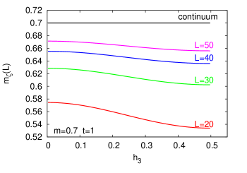
Figure 1: The continuum limit of $m_{\zeta}$ (refer Eq. (50)) at various $h_{3}$ is shown for $m=0.7$ and $t=1$. The spatial lattice extent $L$ is specified on top of each curve. The continuum limit of $m_{\zeta}$ obtained by $1/L$ extrapolation is shown by the topmost black line. This continuum limit matches with $m=0.7$ at all $h_{3}$.

In order to check consistency with the results from zeta function regularization in Deser:1997nv ; Deser:1997gp , we computed $\Gamma$ for several values of $m=ML$ and several values of $t=\frac{L}{\beta}$. For the different $\Gamma$ that we computed at finite $L$, the mass term used in the zeta function regularization would correspond to

$$\frac{m_{\zeta}(L)}{t}=\ln\frac{\tan\Gamma}{\cos 2\pi h_{3}\tan\Gamma-\sin 2\pi h_{3}}.$$ (50)

We extracted the continuum limit of $m_{\zeta}$ by fitting the results for $L=20,22,\cdots,48,50$ using a polynomial in $\frac{1}{L}$. We verified that the extracted value for $m_{\zeta}$ matches with $m$ quite well. Our checks were made in the range $m\in[0.2,1.0]$ and $t\in[0.1,3]$. We show an example of the $L$-dependence of $m_{\zeta}$ in Figure 1 using $m=0.7$ and $t=1$. The continuum limit of $m_{\zeta}$ is seen to match with the $m$ used in our lattice calculation.

IV.2 Uniform and static electric fields

At any finite non-zero temperature and finite volume, it is possible to have spatially uniform and static electric fields, i.e., non-zero $q_{1}$ and $q_{2}$ which are integers. Also, $q_{1}$ and $q_{2}$ need not have the same value. In this subsection, we consider this case of non-zero electric fields, but with no magnetic field. The lattice gauge field background in Eq. (22) reduces to

$$U_{1}({\bf x},k) = e^{i\frac{2\pi q_{2}}{L\beta}k},$$ (51)

$$U_{2}({\bf x},k) = e^{-i\frac{2\pi q_{1}}{\beta L}k},$$ (52)

$$U_{3}({\bf x}) = e^{-i\frac{2\pi q_{2}}{L}x_{1}+i\frac{2\pi q_{1}}{L}x_{2}}.$$ (53)

We focus on the parity even phase arising from this configuration. At any time-slice, the above $U_{1}$ and $U_{2}$ act like time-dependent torons $h_{1}$ and $h_{2}$ whose effect is to offset the momentum. Switching to momentum basis and using the replacement $n_{i}\to n_{i}+h_{i}$, the two dimensional transfer matrix becomes

$${\cal T}_{k}^{n,s}={\cal T}\left(n_{1}+q_{2}\frac{k}{\beta},n_{2}-q_{1}\frac{k}{\beta}\right)\delta_{n_{1},s_{1}}\delta_{n_{2},s_{2}},$$ (54)

where ${\cal T}$ is given by Eq. (42) for the case with torons. The $n$ and $s$ are the momentum indices. The product of these matrices is diagonal in momentum space and it is denoted as $t_{n_{1},n_{2}}$

$$\left[\prod_{k=\beta}^{1}{\cal T}_{k}\right]^{n,s}\equiv\delta^{n_{1},s_{1}}\delta^{n_{2},s_{2}}t_{n_{1},n_{2}}.$$ (55)

Since $T_{3}$ is already in a definite momentum $(-q_{2},q_{1})$, it becomes $\mathbf{1}\delta^{n_{1},s_{1}-q_{2}}\delta^{n_{2},s_{2}+q_{1}}$. Thus,

$$\left[\prod_{k=\beta}^{1}{\cal T}_{k}{\cal T}_{3}\right]^{n,s}=t_{n_{1},n_{2}}\delta^{n_{1}-q_{2},s_{1}}\delta^{n_{2}+q_{1},s_{2}}.$$ (56)

We block-diagonalize the above matrix in the following way. Starting from an arbitrary momentum $(n_{1},n_{2})$, we create a cycle ${\cal C}$ by moving to $(n_{1}-q_{2},n_{2}+q_{1})$, then to $(n_{1}-2q_{2},n_{2}+2q_{1})$ and so on till we are back at $(n_{1},n_{2})$. This will occur after $P$ steps when both $Pq_{2}$ and $Pq_{1}$ become multiples of $L$. We refer to $P$ as the cycle length and this is fixed given $q_{1}$, $q_{2}$ and $L$. The cycle ${\cal C}$ corresponds to a $P\times P$ block, and it has the following structure

$$\left[\prod_{k=\beta}^{1}{\cal T}_{k}{\cal T}_{3}\right]_{\cal C}=\begin{pmatrix}0&t_{n_{1},n_{2}}&0&0&\ldots&0\cr 0&0&t_{n_{1}+q_{2},n_{1}-q_{1}}&0&\ldots&0\cr 0&0&0&t_{n_{1}+2q_{2},n_{1}-2q_{1}}&\ldots&0\cr\vdots&\vdots&\vdots&\vdots&\ldots&\vdots\cr t_{n_{1}+(P-1)q_{2},n_{2}-(P-1)q_{1}}&0&0&0&\ldots&0\end{pmatrix}.$$ (57)

The full momentum space will be split into several such $P\times P$ blocks. If we choose another $(n_{1},n_{2})$ that occurs in the above block as the initial points of the cycle, it will only permute the entries of the block and it will not change the determinant. Thus the full determinant of ${\cal H}$ factorizes into cycles with the factor from each cycle being

$$\left[\det{\cal H}\right]_{\cal C}=\det\left[1-\prod_{r=0}^{P-1}t_{n_{1}-rq_{2},n_{2}+rq_{1}}\right],$$ (58)

which after cyclic permutation of the product of matrices becomes

$$\left[\det{\cal H}\right]_{\cal C}=\det\left[1-\prod_{k=0}^{\beta P}{\cal T}\left(n_{1}-q_{2}\frac{k}{\beta},n_{2}+q_{1}\frac{k}{\beta}\right)\right].$$ (59)

Since products of ${\cal T}$ have unit determinant, it follows that

$$\left[\det{\cal H}\right]_{\cal C}=(1-\rho)\left(1-\frac{1}{\rho}\right),$$ (60)

where $\rho$ is the complex eigenvalue of the product of ${\cal T}$ around a cycle. The eigenvalues $\xi$ of the full transfer matrix are the $P$-th roots of $\rho$ and $1/\rho$ in all the cycles. The complex number $\rho$ characterizes the propagation along a cycle. We will show that there are real cycles where $\rho$ is either real or a complex number with unit magnitude. If the eigenvalue in the real cycle switches sign as a function of mass, then it will be associated with a non-zero contribution to the parity even part of $\Gamma$.

The product of ${\cal T}$ taken along a cycle ${\cal C}$ on the two dimensional momentum torus has the following interpretation. We start with some point $(\frac{n_{1}}{L},\frac{n_{2}}{L})$ on the continuum momentum torus of size $1\times 1$. We move continuously along the direction $(-q_{2},q_{1})$ and compute the fermion propagation along a closed loop in this direction. One can formally convert this into an interpretation in the continuum without worrying about regularization. The integer momenta $(n_{1},n_{2})$ cover the entire range of integers in the continuum. The continuum Hamiltonian in the $\tau$ direction at a fixed $(n_{1},n_{2})$ is

$$\tilde{H}\!\!\!\!/\ (\tau)=-\sigma_{2}\frac{2\pi}{l}\left(n_{1}-q_{2}\tau t\right)+\sigma_{1}\frac{2\pi}{l}\left(n_{2}+q_{1}\tau t\right)+\sigma_{3}m.$$ (61)

We define fermion propagation as

$$\tilde{\phi}(\tau+d\tau)=e^{\tilde{H}\!\!\!\!/\ (\tau)d\tau}\tilde{\phi}(\tau),$$ (62)

in the limit of $d\tau\to 0$. Let $\tilde{\phi}^{\pm}(\infty)$ be the result of propagation from the vector $(1,0)^{t}$ and $(0,1)^{t}$ respectively at $\tau=-\infty$. Then,

$$\left[\det{\cal H}\right]_{\cal C}=\det\left[1-\begin{pmatrix}\tilde{\phi}^{+}(\infty)&\tilde{\phi}^{-}(\infty)\end{pmatrix}\right].$$ (63)

in the continuum.

In order to classify cycles, consider the momenta $(n_{1},n_{2})$ and $(L-n_{1},L-n_{2})$. From the expression for ${\cal T}$ in Eq. (42),

$${\cal T}\left(L-n_{1}-q_{2}\frac{k}{\beta},L-n_{2}+q_{1}\frac{k}{\beta}\right)=\sigma_{3}{\cal T}\left(n_{1}+q_{2}\frac{k}{\beta},n_{2}-q_{1}\frac{k}{\beta}\right)\sigma_{3}.$$ (64)

Using this identity, we now show that if $\rho$ is associated with the $(n_{1},n_{2})$ cycle, $\rho^{*}$ is associated with the $(L-n_{1},L-n_{2})$ cycle. Inserting $\sigma_{3}^{2}$ between the ${\cal T}$’s in Eq. (59), we have

$$\det\left[1-\prod_{k=0}^{\beta P}{\cal T}\left(L-n_{1}-q_{2}\frac{k}{\beta},L-n_{2}+q_{1}\frac{k}{\beta}\right)\right]=\det\left[1-\prod_{k=0}^{\beta P}{\cal T}\left(n_{1}+q_{2}\frac{k}{\beta},n_{2}-q_{1}\frac{k}{\beta}\right)\right].$$ (65)

If we take the complex conjugate of the right hand side, then the product becomes a product of ${\cal T}^{\dagger}$ with the ordering reversed. Using the fact that ${\cal T}$ are hermitean, and after changing the variable $k$ to $\beta P-k$ so as to recover the original ordering (modulo $L$), we obtain

$$\det\left[1-\prod_{k=0}^{\beta P}{\cal T}\left(L-n_{1}-q_{2}\frac{k}{\beta},L-n_{2}+q_{1}\frac{k}{\beta}\right)\right]=\left\{\det\left[1-\prod_{k=0}^{\beta P}{\cal T}\left(n_{1}-q_{2}\frac{k}{\beta},n_{2}+q_{1}\frac{k}{\beta}\right)\right]\right\}^{*}.$$ (66)

This completes the proof.

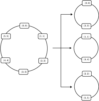
Figure 2: On the left is the real cycle ${\cal R}_{0}$ with coprime steps $q_{1}=q_{2}=1$ on a $6^{3}$ lattice. This cycle has a length $P=6$. When $q_{1}=q_{2}=3$, the cycle ${\cal R}_{0}$ splits into 3 cycles each of length $P=2$.

We classify cycles in the following way. The cycles ${\cal C}$ and ${\cal C}^{*}$ are conjugate if $(n_{1},n_{2})$ and $(L-n_{1},L-n_{2})$ belong to ${\cal C}$ and ${\cal C}^{*}$ respectively. If ${\cal C}$ and ${\cal C}^{*}$ are the same cycle, then we call it a real cycle and denote it by ${\cal R}$. If the cycle is real then we have

$$\left[\det{\cal H}\right]_{\cal R}=(1-\rho)\left(1-\frac{1}{\rho}\right)=(1-\rho^{*})\left(1-\frac{1}{\rho^{*}}\right).$$ (67)

This implies that either $\rho$ is real or $\rho$ is a complex number with unit magnitude. Since the eigenvalues of conjugate cycles are related by complex conjugation, they can be paired together to give a positive contribution to $\det{\cal H}$. Therefore, only the real cycles contribute to the phase, which can only be $\pm 1$. The following cases are possible for the real cycles.

1. When $\rho=e^{i\phi}$, the factor will be real and positive in the above product.

2. When $\rho$ is real and negative, the contribution will be positive.

3. When $\rho$ is real and positive, the contribution will be negative.

Depending on the number of real cycles in the above categories, the phase could be either $+1$ or $-1$. Let us start by assuming that $q_{1}$ and $q_{2}$ are coprimes. All the cycles have the same length, $P$, which is even for even $L$. Let us assume that $(n_{1},n_{2})$ belongs to a real cycle. Since $(L-n_{1},L-n_{2})$ belongs to the same cycle, it follows that

$$\left(L-n_{1},L-n_{2}\right)=\left(n_{1}-rq_{2},n_{2}+rq_{1}\right)+\left(k_{1}L,k_{2}L\right),$$ (68)

for some integers $r$, $k_{1}$ and $k_{2}$. Since $q_{1}$ and $q_{2}$ are coprimes and $L$ is assumed to be even, it follows that $r$ is even and

$$\left(n_{1}-\frac{r}{2}q_{2},n_{2}+\frac{r}{2}q_{1}\right)=\left((1-k_{1})\frac{L}{2},(1-k_{2})\frac{L}{2}\right).$$ (69)

Therefore, real cycles have to contain $(n_{1},n_{2})=(0,0)$, $\left(\frac{L}{2},0\right)$, $\left(0,\frac{L}{2}\right)$ or $\left(\frac{L}{2},\frac{L}{2}\right)$. Let ${\cal R}_{0}$ denote the cycle that contains $(n_{1},n_{2})=(0,0)$. For every $(-rq_{2},rq_{1})$ in this cycle there is a partner, $(rq_{2},-rq_{1})$, in the cycle. Only $(0,0)$, $\left(\frac{L}{2},0\right)$, $\left(0,\frac{L}{2}\right)$ or $\left(\frac{L}{2},\frac{L}{2}\right)$ have themselves as their partner. Since each cycle has an even number of points, we conclude that one of $\left(\frac{L}{2},0\right)$, $\left(0,\frac{L}{2}\right)$ or $\left(\frac{L}{2},\frac{L}{2}\right)$also belongs to ${\cal R}_{0}$. Since the length $P$ can have only one factor of $2$, the number of cycles, $\frac{L^{2}}{P}$ has to be even. Since the complex cycles pair up, the two left over from $\left(\frac{L}{2},0\right)$, $\left(0,\frac{L}{2}\right)$ and $\left(\frac{L}{2},\frac{L}{2}\right)$ have to pair up and belong to another real cycle, which we call ${\cal R}_{\pi}$. If $q_{1}$ and $q_{2}$ have a common factor, then we will assume that we choose a set of $L$ that all have this factor while taking the continuum limit. Under such a choice, the common factor of $q_{1}$, $q_{2}$ and $L$ can be pulled out resulting in multiples of cycles traced using coprime steps $q_{1}$ and $q_{2}$ on a smaller spatial lattice. For the sake of clarity, we demonstrate the above statement in Figure 2, for the case $q_{1}=q_{2}=3$ on a $6^{3}$ lattice.

We now numerically show that the phase for ${\cal R}_{0}$ is $0$ and ${\cal R}_{\pi}$ is $\pi$ for all values of $q_{1}$ and $q_{2}$ that are coprime. This enables us to write the continuum formula for the phase for this case as

$$\Gamma_{\rm even}=\pi(q_{1}+q_{2}+q_{1}q_{2}),$$ (70)

in accordance with Eq. (15). In order to maintain numerical stability in the computation of the product of transfer matrices in Eq. (59), we found it useful to normalize each row separately as we multiply and cumulate the normalization factors in a single diagonal matrix. Using this procedure we were able to work with large $L$ and $\beta$, thereby essentially seeing the behavior of cycles in the continuum limit. The top left panel in Figure 3 shows the flow of the phase from each cycle as a function of mass when the background electric flux is $q_{1}=2$ and $q_{2}=3$. The flow is close to what one would see in the continuum since the computations are on a $160^{3}$ lattice. The phase from the real cycle ${\cal R}_{0}$ changes from being $\pi$ for $m<m_{c}(L)$ to $0$ for $m>m_{c}(L)$ for some positive $m_{c}(L)$, which becomes zero in the continuum limit as shown in the top right panel of Figure 3. The real cycle ${\cal R}_{\pi}$ has a phase of $\pi$ for all masses. The rest of the cycles are complex and come in pairs as is evident from the plot. The combined phase is only due to the real cycles and is $\pi$ for all masses above $m_{c}(L)$. This is consistent with Eq. (70).

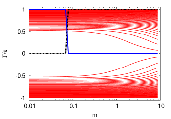
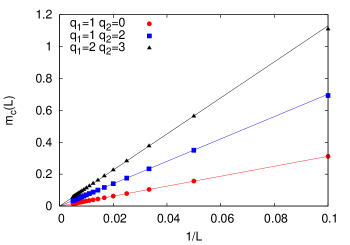
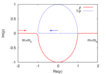
Figure 3: The flow of phase from each cycle as a function of mass for a background with fixed electric flux. Top left panel: The flow for all cycles with $q_{1}=2$, $q_{2}=3$ on $160^{3}$ lattice is shown as red lines. The real cycle ${\cal R}_{0}$ is shown by the solid blue line. In addition the plot shows the overall phase as a black dotted line. It is obvious through a visual inspection that the eigenvalues occur as complex conjugate pairs. The phase of the real cycle, and hence the overall phase, jump at an $m_{c}$ (the points are only connected to aid the eye). Top right panel: The lattice spacing dependence of $m_{c}$ is shown for various values of $q_{1}$ and $q_{2}$. In the continuum limit, $L\to\infty$, the $m_{c}$ vanishes. Bottom panel: Flow of eigenvalues of the real cycle seen on the complex plane, in the region of crossing around $m_{c}$. The plot corresponds to flux $q_{1}=1$, $q_{2}=0$ on $4^{3}$ lattice in the region $0.188138<m<0.188144$. The pair of eigenvalues $\left(\rho,\frac{1}{\rho}\right)$ flow from real negative values for $m>m_{c}$ to a complex pair of unit magnitude, and finally to real positive values.

It is interesting to focus on the crossing that occurs in the ${\cal R}_{0}$ cycle. In order to zoom in on the crossing, it is better to work on a coarse lattice and we picked $q_{1}=1$ and $q_{2}=0$ on a $4^{3}$ lattice and considered $m\in[0.188138,0.188144]$. We look at the eigenvalue pair $\left(\rho,\frac{1}{\rho}\right)$ as the mass is changed in this very small range. The flow of eigenvalues on the complex plane is shown on the bottom panel of Figure 3. The eigenvalue pair starts out being positive on the low end of the mass region and approach unity at some $m_{c}$ which lies within the range. For a range of $m$ above $m_{c}$, $\rho$ and $\frac{1}{\rho}$ trace a $|\rho|=1$ locus on the complex plane. Finally, the $\rho$ becomes real and less than zero. The background with $q_{1}=1$ and the one with $q_{3}=1$ are related by a rotation. Thus, the zero crossing of an eigenvalue $\lambda^{+}$ in the latter case, can now be equivalently understood as the flip in the sign of $\rho$ of the cycle containing the zero mode. The range of $m$ where this behavior occurs shrinks dramatically as one approaches the continuum and the value of $m_{c}$ gets closer to zero.

As explained, when $q_{1}$ and $q_{2}$ are not coprimes, the cycles split into $N$ cycles each, ($N=3$ in the example shown in Figure 2) depending on the values of $q_{1}$ and $q_{2}$. Thus, all the $N$ cycles originating from ${\cal R}_{0}$ result in a phase that switches from $\pi$ to zero as $m$ crosses $m_{c}$ from below. The other $N$ cycles originating from ${\cal R}_{\pi}$ always have a phase of $\pi$. Thus, the total phase becomes

$$\Gamma=\pi(N{\rm mod\ }2).$$ (71)

Only when both $q_{1}$ and $q_{2}$ are even, $N$ can be even. Thus the expression for the phase remains as Eq. (70) even when $q_{1}$ and $q_{2}$ are not coprime.

Now we proceed to add $h_{1}$ and $h_{2}$ to the gauge field background in Eq. (53). The effect is to replace $n_{i}$ by $n_{i}+h_{i}$ in Eq. (59):

$$\left[\det{\cal H}\right]_{\cal C}=\det\left[1-\prod_{k=0}^{\beta P}{\cal T}\left(n_{1}+h_{1}-q_{2}\frac{k}{\beta},n_{2}+h_{2}+q_{1}\frac{k}{\beta}\right)\right].$$ (72)

The full determinant still factorizes into cycles but the real cycles now become complex and the previous complex cycles that were complex conjugate pairs are no longer paired. If $h_{1}$ and $h_{2}$ are multiples of $q_{2}/\beta$ and $q_{1}/\beta$ respectively, then it is possible to find an integer $k^{\prime}=k-\frac{\beta h_{1}}{q_{2}}$, such that the determinant becomes

$$\left[\det{\cal H}\right]_{\cal C}=\det\left[1-\prod_{k^{\prime}=0}^{\beta P}{\cal T}\left(n_{1}-q_{2}\frac{k^{\prime}}{\beta},n_{2}+\frac{h_{1}q_{1}+h_{2}q_{2}}{q_{2}}+q_{1}\frac{k^{\prime}}{\beta}\right)\right].$$ (73)

This means that at any fermion mass and temperature, the phase can only be a function of $h_{1}q_{1}+h_{2}q_{2}$. In the continuum limit, the fact that we chose a rational $h_{1}$ and $h_{2}$ should not matter. We proceed to compute the phase per cycle and the total parity odd part of the phase of the determinant numerically in order to understand the term in the phase that couples $h_{i}$ with $q_{i}$. Two sample cases studied are plotted in Figure 4. Consider the case of $q_{1}=1$ and $q_{2}=0$ with $h_{1}=0.23$ and $h_{2}=0$ shown on the left panel of Figure 4. This is just a rotated version of the case with constant magnetic flux and a temporal toron. After removing a factor of $-1$ from the determinant due to the parity even part of the phase, the parity odd part of the phase at the largest mass is consistent with $-2\pi h_{1}q_{1}$ as expected from Eq. (49). Next, we consider the more interesting case of $q_{1}=2$, $q_{2}=3$ with $h_{1}=0.37$ and $h_{2}=0.23$ shown on the right panel of Figure 4. The parity even part of the phase is again $\pi$ as in the previous case. The parity odd part of the phase at the largest mass is consistent with

$$\Gamma=-2\pi(h_{1}q_{1}+h_{2}q_{2}),$$ (74)

which is indicated by arrows in the plots.

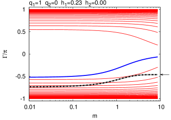
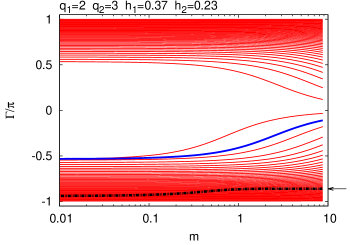
Figure 4: The flow of phase from all the cycles (red lines) as a function of mass on a background with fixed electric fluxes and torons. The left panel shows this flow for a background with flux $q_{1}=1$, $q_{2}=0$ and torons $h_{1}=0.23$, $h_{2}=0$ on $160^{3}$ lattice. Similarly, the right panel is for a background with flux $q_{1}=2$, $q_{2}=3$ and torons $h_{1}=0.37$, $h_{2}=0.23$. The cycle that would have been the real cycle ${\cal R}_{0}$ when torons are absent, is specially shown by the solid blue line. The overall parity odd part of the phase as black dashed line. The arrows indicate the expectations from Eq. (74) for the infinite mass limit.

IV.3 Uniform and static electric and magnetic fields

$\quad q_{1}\quad$	$\quad q_{2}\quad$	$\quad q_{3}\quad$	$\quad\Gamma/\pi\quad$
0	0	0	0
0	0	1	1
0	1	0	1
0	1	1	1
1	0	0	1
1	0	1	1
1	1	0	1
1	1	1	0

Table 1: Phase $\Gamma$ for various combinations of $q_{1}$, $q_{2}$ and $q_{3}$. The “0” represents even integers and “1” represents odd integers.

Now we consider the gauge field background where electric as well as magnetic fields are present i.e., $q_{1}$, $q_{2}$ and $q_{3}$ terms are all present in Eq. (22) with no torons. We are unable to study this case analytically. Therefore, we study this general case by directly evaluating Eq. (36). We check for any loss of precision by comparing the determinant of the product of ${\cal T}_{k}$ to 1. Doing so, we were able to use up to $12^{3}$ lattices. We find that $\det D$ is real for any $q_{1}$, $q_{2}$ and $q_{3}$. Thus, the phase can only be $\pm 1$ and its expression must be of the form

$$\Gamma=\eta_{1}\pi\left(q_{1}+q_{2}+q_{3}\right)+\eta_{2}\pi\left(q_{1}q_{2}+q_{2}q_{3}+q_{3}q_{1}\right)+\eta_{3}\pi q_{1}q_{2}q_{3},$$ (75)

where $\eta_{i}=0$ or 1. Rotational symmetry guarantees that each $\eta_{i}$ are the same for all directions. From the last section, we know that $\eta_{1}=\eta_{2}=1$. We do not have any analytical argument about $\eta_{3}$. In Table 1, we collect our observations about the dependence of phase on $q_{1}$, $q_{2}$ and $q_{3}$. The results of the table are robust and found to be the same on $L=$4, 6, 8, 10 and 12 lattices, and for various even and odd values for the $q$’s. The entries with $q_{3}=0$ reiterate our observations of the last subsection. The entry with even $q_{1}$ and $q_{2}$ includes the case $q_{1}=q_{2}=0$, which we understand as due to the mismatch between the number of positive and negative eigenvalues of a two dimensional Dirac operator. The other cases do not offer a simple analytical explanation. The important entry is the last one where all $q$’s are odd. Since the phase is even, it implies that $\eta_{3}=0$. Thus, $\det D$ has a parity even phase given by

$$\Gamma=\pi\left(q_{1}+q_{2}+q_{3}\right)+\pi\left(q_{1}q_{2}+q_{2}q_{3}+q_{3}q_{1}\right).$$ (76)

V Perturbation theory: Parity odd contributions

In this section, we return to the case of uniform and static magnetic field in the presence of a uniform toron in the Euclidean time direction that was studied in Section IV.1 and consider perturbations $A_{1}^{p}$ and $A_{2}^{p}$ on this background. We expand the determinant for ${\cal H}$ in Eq. (36) in powers of $A^{p}_{i}$ while considering the constant flux background and the toron to be non-perturbative. The transfer matrix, ${\cal T}_{k}$, can be expanded to second order in $A_{i}^{p}$ as

$${\cal T}_{k}={\cal T}+{\cal F}_{k}+{\cal S}_{k}.$$ (77)

The detailed expressions for ${\cal F}_{k}$ and ${\cal S}_{k}$ are given in Appendix A. We write

$$\prod_{k=\beta}^{1}{\cal T}_{k}={\cal T}^{\beta}\left[1+P\right],$$ (78)

where

$$P=\sum_{k=0}^{\beta-1}{\cal T}^{-k-1}{\cal F}_{k+1}{\cal T}^{k}+\sum_{k=0}^{\beta-1}{\cal T}^{-k-1}{\cal S}_{k+1}{\cal T}^{k}+\sum_{k=1}^{\beta-1}\sum_{l=0}^{k-1}{\cal T}^{-k-1}{\cal F}_{k+1}{\cal T}^{k-l-1}{\cal F}_{l+1}{\cal T}^{l}.$$ (79)

From Eq. (36), we have

$$\log\det{\cal H}=\log\det{\cal H}_{\rm st}+\log\det\left[1+{\cal H}_{\rm st}^{-1}PT_{3}^{\dagger}\right].$$ (80)

Using standard perturbation theory in the eigenbasis of the unperturbed ${\cal T}$, we arrive at

$$\log\det\left[1+{\cal H}_{\rm st}^{-1}PT_{3}^{\dagger}\right] = \sum_{i\pm}\sum_{k=0}^{\beta-1}\frac{e^{\pm(\beta-1)\lambda_{i}^{\pm}-i2\pi h_{3}}}{1+e^{\pm\beta\lambda_{i}^{\pm}-i2\pi h_{3}}}{\cal F}_{k+1}^{i\pm,i\pm}+\sum_{i\pm}\sum_{k=0}^{\beta-1}\frac{e^{\pm(\beta-1)\lambda_{i}^{\pm}-i2\pi h_{3}}}{1+e^{\pm\beta\lambda_{i}^{\pm}-i2\pi h_{3}}}{\cal S}_{k+1}^{i\pm,i\pm}$$ (83)

$$-\frac{1}{2}\sum_{i\pm}\sum_{j\pm}\sum_{k=0}^{\beta-1}\frac{e^{\pm(\beta-1)\lambda_{i}^{\pm}\pm(\beta-1)\lambda_{j}^{\pm}-i4\pi h_{3}}}{\left(1+e^{\pm\beta\lambda_{i}^{\pm}-i2\pi h_{3}}\right)\left(1+e^{\pm\beta\lambda_{j}^{\pm}-i2\pi h_{3}}\right)}{\cal F}_{k+1}^{i\pm,j\pm}{\cal F}_{k+1}^{j\pm,i\pm}$$

$$+\sum_{i\pm}\sum_{j\pm}\sum_{k=1}^{\beta-1}\sum_{l=0}^{k-1}\frac{e^{\pm(\beta-k+l-1)\lambda_{i}^{\pm}\pm(k-l-1)\lambda_{j}^{\pm}-i2\pi h_{3}}}{\left(1+e^{\pm\beta\lambda_{i}^{\pm}-i2\pi h_{3}}\right)\left(1+e^{\pm\beta\lambda_{j}^{\pm}-i2\pi h_{3}}\right)}{\cal F}_{k+1}^{i\pm,j\pm}{\cal F}_{l+1}^{j\pm,i\pm}+{\cal O}(A^{3}),$$

where it is implicit that the summation over $i+$ runs up to $V+q_{3}$, while that of $i-$ up to $V-q_{3}$. We use this general second order perturbative expression to study two cases of interest.

V.1 Zero temperature

We assume that we are working away from the massless limit and therefore $\lim_{L\to\infty}L\lambda_{i}^{\pm}$ are strictly greater than zero for all $i$. Since $\beta=\frac{L}{t}$, we see that in the limit $t\to 0$, the first three terms in Eq. (83) are real and do not contribute to the phase. The last term can be simplified as follows. Let

$$\left|{\cal F}_{k+1}^{i\pm,j\pm}{\cal F}_{l+1}^{j\pm,i\pm}\right|<X^{i\pm,j\pm},$$ (84)

where the upper-bound $X^{i\pm,j\pm}$ is independent of $\beta$. Then, the sum is bounded above by

$$Y_{i\pm,j\pm}(\beta)=\frac{e^{\pm(\beta-1)\lambda_{i}^{\pm}-i2\pi h_{3}}}{1+e^{\pm\beta\lambda_{i}^{\pm}-i2\pi h_{3}}}\frac{1}{1+e^{\pm\beta\lambda_{j}^{\pm}-i2\pi h_{3}}}\frac{\beta\left(1-e^{\pm\lambda^{\pm}_{j}\mp\lambda^{\pm}_{i}}\right)+\left(1-e^{\beta\left(\pm\lambda^{\pm}_{j}\mp\lambda^{\pm}_{i}\right)}\right)}{2\left(\cosh\left(\pm\lambda^{\pm}_{j}\pm\lambda^{\pm}_{i}\right)-1\right)}X^{i\pm,j\pm}.$$ (85)

Explicitly, $Y_{i+,\j+}$ and $Y_{i-,j-}$ vanish in the $\beta\to\infty$ limit. Therefore, we need to consider only the products of ${\cal F}^{i+,j-}_{k+1}$ and ${\cal F}^{i-,j+}_{l+1}$ terms. The phase is

$$\Gamma=\pi q_{3}-2\pi h_{3}q_{3}+\lim_{\beta\to\infty}\sum_{i=1}^{V+q_{3}}\sum_{j=1}^{V-q_{3}}e^{\left(\lambda_{j}^{-}-\lambda_{i}^{+}\right)}\sum_{k=1}^{\beta-1}\sum_{l=0}^{k-1}\left(e^{(l-k)\left(\lambda_{i}^{+}+\lambda_{j}^{-}\right)}-e^{(k-l-\beta)(\lambda_{i}^{+}+\lambda_{j}^{-})}\right){\rm\ Im\ }{\cal F}^{i+,j-}_{k+1}{\cal F}^{j-,i+}_{l+1}.$$ (86)

The second term does not depend on $h_{3}$ and therefore the contribution from the toron $h_{3}$ and the perturbative part are independent of each other at this order. If we assume $\frac{k-l}{L}$ is kept finite in the infinite $L$ limit, then we can ignore the second factor in the parenthesis of the second term. The term $2\pi q_{3}h_{3}$ is independent of $m$ and changes in multiples of $2\pi$ under large gauge-transformation $h_{3}\to h_{3}+1$. Even at zero temperature, the induced gauge action is not of the type in Eq. (2) if we include fields that do not vanish at infinity.

V.2 Finite temperature and $\mathbf{h_{3}=0}$

Our aim in this subsection is to study the purely perturbative contribution to the phase in a possibly non-perturbative background at finite temperature. Since we are focusing on terms of the type, $A_{1}^{p}A_{2}^{p}$, we set $h_{3}=0$. In addition we only consider $A_{1}^{p}(k)$ and $A_{2}^{p}(k)$ that depend only on time. When $h_{3}=0$, the first three terms in Eq. (83) are real even at finite $\beta$. The phase becomes

$$\Gamma=\sum_{i\pm}\sum_{j\pm}\sum_{k=1}^{\beta-1}\sum_{l=0}^{k-1}\frac{e^{\pm(\beta-k+l-1)\lambda_{i}^{\pm}\pm(k-l-1)\lambda_{j}^{\pm}}}{\left(1+e^{\pm\beta\lambda_{i}^{\pm}}\right)\left(1+e^{\pm\beta\lambda_{j}^{\pm}}\right)}{\rm Im}{\cal F}_{k+1}^{i\pm,j\pm}{\cal F}_{l+1}^{j\pm,i\pm}.$$ (87)

After writing

$${\cal F}^{i\pm,j\pm}_{k}=\sum_{\mu=1}^{2}\widetilde{\cal F}^{i\pm,j\pm}_{\mu}A_{\mu}^{p}(k),$$ (88)

we arrive at an expression for the phase, which is written concisely as

$$\Gamma=-\sum_{k=1}^{\beta-1}\sum_{l=0}^{k-1}G(k-l)\left[A^{p}_{1}(k)A^{p}_{2}(l)-A^{p}_{2}(k)A^{p}_{1}(l)\right].$$ (89)

The form factor $G$ is

$$G(k)=\sum_{(i\pm,j\pm)}e^{\mp\lambda_{i}^{\pm}\mp\lambda_{j}^{\pm}}\frac{\sinh\left[\left(\frac{\beta}{2}-k\right)(\pm\lambda_{i}^{\pm}\mp\lambda_{j}^{\pm})\right]}{4\cosh\frac{\beta\lambda_{i}^{\pm}}{2}\cosh\frac{\beta\lambda_{j}^{\pm}}{2}}{\rm Im}\left[\left(\widetilde{\cal F}_{1}^{i\pm,j\pm}\right)^{*}\widetilde{\cal F}_{2}^{i\pm,j\pm}\right].$$ (90)

It satisfies the anti-symmetric property

$$G(\beta-k)=-G(k).$$ (91)

This expression is valid for all $q_{3},h_{1}$ and $h_{2}$. For the free case $q_{3}=0$ that we discussed in Section III.1, the form factor simplifies to

$$G(k)=\sum_{p}\frac{\sinh\left[\left(\beta-2k\right)\lambda_{p}\right]}{2\cosh^{2}\frac{\beta\lambda_{p}}{2}}{\rm Im}\left[\left(\widetilde{\cal F}_{1}^{p+,p-}\right)^{*}\widetilde{\cal F}_{2}^{p+,p-}\right].$$ (92)

We derive the expressions for ${\cal F}^{p+,p-}_{\mu}$ in Appendix B.

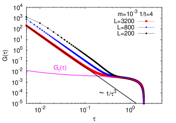
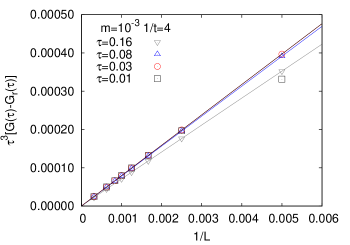
Figure 5: Left panel: The form factor $G(\tau)$ at fermion mass $m=10^{-3}$ is shown at a temperature $t=0.25$ for the free $q_{3}=0$ background gauge-field with no torons. The different symbols correspond to different $L$. At all $L$, $G(\tau)$ shows a $\tau^{-3}$ behaviour at small values of $\tau$. The best fit for this power-law $\tau^{-3}$ using the $L=3200$ data are shown as the black straight line. When the continuum is approached by increasing $L$, the power-law behaviour shifts to the left on the log-log plot such that $G(\tau)$ approaches $G_{r}(\tau)$ (refer Eq. (95)) at all $\tau$. This continuum limit $G_{r}(\tau)$ is shown as the magenta curve. Right panel: The approach to continuum of the scaled variable $\tau^{3}\left[G(\tau)-G_{r}(\tau)\right]$ is shown at various $\tau$. At all $\tau$, it approaches 0 with a dominant $\frac{1}{L}$ scaling. For very small $\tau$, there is data collapse suggesting a perfect $\tau^{-3}$ scaling. At larger $\tau$, there are corrections to this scaling. However, it is the most singular $\tau^{-3}/L$ behaviour of $G(\tau)$ that is important to the phase of $\det D$.

The behavior of this form factor $G$ is shown as a function of time $\tau=\frac{k}{L}$ in Figure 5. The observations about the long and short distance behaviour of $G(\tau)$ seen in the two panels of the figure can be summarized in the following way. The $G(\tau)$ has a leading $\frac{1}{L}$ lattice correction. However, the coefficient of $\frac{1}{L}$ shows a singular $\tau^{-3}$ behaviour. That is, the approach to the continuum limit is given by

$$G(\tau L)=G_{r}(\tau)+\frac{1}{L}G_{s}(\tau)+{\cal O}\left(\frac{1}{L^{2}}\right),$$ (93)

where $G_{r}(\tau)$ is the continuum limit, while the singular coefficient of the dominant $\frac{1}{L}$ correction is given by

$$G_{s}(\tau)=\frac{f(m,t)}{\tau^{3}}+{\cal O}\left(\tau^{-2}\right),$$ (94)

for some mass and temperature dependent function $f$. The continuum limit, $G_{r}(\tau)$, seems to be well described by the regulator independent limit obtained by replacing $\lambda_{p}L$ by its $p\approx 0$ limit, $\Lambda_{p}$ i.e.,

$$G_{r}(\tau)=\sum_{n}\frac{m}{\Lambda_{n}}\frac{\sinh\left[\left(\frac{1}{t}-2\tau\right)\Lambda_{n}\right]}{2\cosh^{2}\left[\frac{\Lambda_{n}}{2t}\right]},$$ (95)

making use of

$$\Lambda_{n}\equiv\lim_{L\to\infty}L\lambda_{p}=\sqrt{m^{2}+4\pi^{2}(n_{1}^{2}+n_{2}^{2})}\qquad\text{and}\qquad\lim_{L\to\infty}{\rm Im}\left[\left(\widetilde{\cal F}_{1}^{p+,p-}\right)^{*}\widetilde{\cal F}_{2}^{p+,p-}\right]=\frac{m}{\Lambda_{n}},$$ (96)

for all momenta even though they only hold true for $p_{i}\approx 0$. The above observations about $G$ are seen at all mass and temperature.

Let us consider the following perturbative fields chosen such that there is a non-zero Chern-Simons action:

$$A^{p}_{1}(k)=\frac{c}{L}\sin\left(\frac{2\pi n_{3}k}{\beta}\right)\qquad\text{and}\qquad A^{p}_{2}(k)=\frac{c}{L}\cos\left(\frac{2\pi n_{3}k}{\beta}\right).$$ (97)

The phase becomes

$$-\frac{\Gamma}{c^{2}}=\lim_{L\to\infty}\frac{1}{L^{2}}\sum_{k=1}^{\beta-1}(\beta-k)G(k)\sin\left(\frac{2\pi n_{3}k}{\beta}\right)=\lim_{L\to\infty}\frac{\beta}{L^{2}}\sum_{k=1}^{\frac{\beta}{2}}G(k)\sin\left(\frac{2\pi n_{3}k}{\beta}\right),$$ (98)

where we have made a change of variable from $k$ and $l$ to $k-l$, and used the antisymmetry property of $G(k)$ in Eq. (91). Inserting Eq. (93) for $G(k)$, we obtain

$$-\frac{\Gamma}{c^{2}}=\lim_{L\to\infty}\frac{\beta}{L^{2}}\sum_{k=1}^{\beta-1}G_{r}(k)\sin\left(\frac{2\pi n_{3}k}{\beta}\right)+\lim_{L\to\infty}\beta\sum_{k=1}^{\frac{\beta}{2}}\frac{f(m,t)}{k^{3}}\sin\left(\frac{2\pi n_{3}k}{\beta}\right).$$ (99)

The first term arising from the continuum part of $G(\tau)$ can be converted to an integral. The second term that arises from the singular part contributes in the continuum due to the $\tau^{-3}$ behavior. The two terms can be expressed as

$$-\frac{\Gamma}{c^{2}}=\frac{1}{t}\int_{0}^{\frac{1}{2t}}G_{r}(\tau)\sin\left(2\pi n_{3}\tau t\right)d\tau+2\pi n_{3}f(m,t)\zeta(2).$$ (100)

The second term is proportional to the momentum $n_{3}$ and hence it is indeed the local Chern-Simons term. It contributes both in the infinite mass and massless limit showing that the parity odd contribution is regulator dependent Redlich:1983dv ; Coste:1989wf . At very low but non-zero temperatures, the contribution from the first term behaves as

$$\frac{\Gamma_{\rm reg}}{c^{2}}\approx-\frac{\pi n_{3}}{2}\sum_{n_{1},n_{2}=0}^{\infty}\frac{m\left(1-e^{-\frac{2\Lambda_{\widetilde{n}}}{t}}\right)}{\Lambda_{\widetilde{n}}\left[\Lambda_{\widetilde{n}}^{2}+n_{3}^{2}\pi^{2}t^{2}\right]}\qquad\text{where}\qquad\widetilde{n_{i}}=n_{i}+h_{i},$$ (101)

after integration over $\tau$. This right away makes it explicit the dependence of the phase on the torons $h_{1}$ and $h_{2}$ in the $q_{3}=0$ background. When the torons are absent, this infinite sum suffers from an infra-red divergence when $t\to 0$ limit is taken before the $m\to 0$ limit. But the sum becomes zero when the two limits are interchanged. In the $m\to\infty$ limit, the infinite sum always vanishes. Thus, the phase from the regular term is zero in both the infinite and zero mass limits and only the singular part contributes to the parity odd phase in these two limits. At any finite and non-zero mass the contribution from the regular term is not local since it is not linear in $n_{3}$.

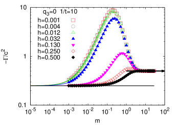
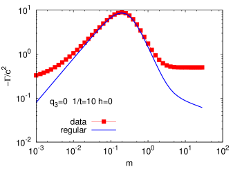
Figure 6: The cross-over of phase from the $m\to 0$ limit (which is $\Gamma=-\frac{c^{2}}{4}$) to the $m\to\infty$ limit ($\Gamma=-\frac{c^{2}}{2}$) when $q_{3}=0$. On the left panel, the mass dependence of $\Gamma$ is shown for various values of $h_{1}=h_{2}=h$ specified by different symbols. For large values of mass ($m\gtrsim 10$), the phase is $-\frac{c^{2}}{2}$. For small values of mass, the phase approaches $-\frac{c^{2}}{4}$ as seen by extrapolation (solid lines) using data points with $m<0.1$. On the right panel, the phase $\Gamma$ (red squares) and the phase calculated only using $G_{r}(\tau)$ (blue line) are compared when $h=0$.

The above discussion shows where the parity breaking phase arises at different masses. We now present results on the phase directly calculated using Eq. (89). On the left panel of Figure 6, we show the behaviour of the phase as a function of fermion mass, for the perturbation in Eq. (97) on a $q_{3}=0$ background. We show the behavior at various values of $h_{1}=h_{2}=h$, and at a temperature $t=0.1$. We did the numerical calculation using lattices with $L=$ 60, 80, 100, 120, 140 and 160. With these, we did a continuum extrapolation for $\Gamma$ using a fourth order polynomial in $\frac{1}{L}$. Changing the order of the polynomial to 3 or 5 made little difference to the results. In the figure, we show these continuum extrapolated values. When $m\to\infty$, the phase becomes $-\frac{c^{2}}{2}$ which is consistent with a Chern-Simons coefficient $\kappa=-1$. Using the values of phase for $m<0.1$, we extrapolated the results to $m=0$ using a fourth order polynomial in $m$. These extrapolations are shown by the solid lines. The extrapolated curves smoothly approach $-\frac{c^{2}}{4}$ as $m\to 0$, independent of $h$. This corresponds to a Chern-Simons coefficient $\kappa=-\frac{1}{2}$, which is consistent with Coste:1989wf . At other intermediate values of $m$, we find a strong dependence on $h_{1}$ and $h_{2}$, which is expected from the above discussions for the $q_{3}=0$ case. From the right panel of Figure 6, it is clear that the toron dependence of the phase indeed comes from $G_{r}(\tau)$. As $t$ becomes smaller, the peak gets higher and shifts to smaller values of $m$ according to Eq. (101).

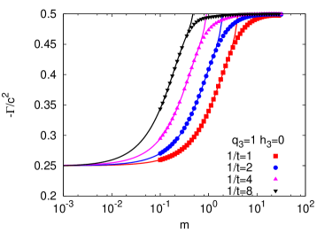
Figure 7: The mass dependence of phase $\Gamma$ with a flux $q_{3}=1$ in the $xy$-plane. The different symbols correspond to various temperatures $t$ which ranges from 1 to $\frac{1}{8}$. The solid lines show the polynomial extrapolation of the phase from small $m<0.1$ to $m=0$. It is seen that the phase approaches $-\frac{1}{2}$ at large mass and the extrapolation shows that the phase approaches $-\frac{1}{4}$ when $m\to 0$.

In Figure 7, we show a similar plot for a $q_{3}=1$ background. We do not find any dependence on the spatial torons. Therefore, we show only the result with $h_{1}=h_{2}=0$. The different symbols are the continuum extrapolated results at four different temperatures. Using a similar procedure as in the $q_{3}=0$ case, we find the phase to be $-\frac{c^{2}}{2}$ and $-\frac{c^{2}}{4}$ in the infinite and zero mass limits respectively. At finite values of $m$, there is a smooth cross-over between the two limits. At smaller $t$, this cross-over occurs at smaller values of $m$, well described by an $\frac{m}{t}$ dependence of the phase.

The above mass dependence is clearly $h_{1}$, $h_{2}$ and $q_{3}$ dependent. Although implicit, one could consider them as $h_{i}-A^{p}_{i}$ and $q_{3}-A^{p}_{i}$ terms in the induced gauge action, that originates from the infra-red and would not be predicted by a pure Chern-Simons term.

VI Conclusions

We studied the contribution to the phase of the fermion determinant in QED₃ using lattice regularization and Wilson fermions at finite volume and temperature. We considered non-perturbative backgrounds that contain non-zero magnetic and electric flux. In addition, our backgrounds also contained constant gauge potentials referred to as torons. In the absence of torons and any perturbation, we studied the parity even contribution to the phase and our result in Eq. (15) is an extension of the result in Forte:1986em ; Forte:1987kj ; AlvarezGaume:1984nf for the case of just a magnetic flux. In the presence of toron in the time direction and a non-zero magnetic flux, our result using lattice regularization agrees with one obtained using zeta function regularization Deser:1997gp ; Deser:1997nv . We extend this result for the case with electric fluxes and torons. In addition to extending the result, we provide an alternate way of understanding the parity even contribution when one has a magnetic flux. The connection between two dimensional topology and a parity even phase is translated to a sign associated with the propagation of a free fermion along a closed loop in two dimensional momentum torus where the momentum associated with the propagation changes as one goes along the closed loop. The direction associated with the closed loop in the two dimensional momentum torus is proportional $(-q_{2},q_{1})$, the fluxes associated with the electric field.

The effect of finite temperature on the coefficient of the induced Chern-Simons term discussed in the past Dunne:1998qy is addressed here. In addition we also address the issue of finite mass. We show that the contribution at zero mass and infinite mass only comes from the regulator but there is also a contribution from the continuum part at non-zero finite masses. Whereas the contribution from the regulator is local and of the Chern-Simons type with a coefficient that is different at zero and infinite mass Coste:1989wf , the contribution at any finite non-zero mass is not local. In addition, the result depends on the presence of torons in the space directions if there is no magnetic flux. This is associated with the eigenvalues of the free two dimensional Dirac operator depending on the torons and the eigenvalues of the two dimensional Dirac operator in the presence of a non-zero magnetic flux being independent of the torons Sachs:1991en .

Our studies in various non-perturbative backgrounds suggest that we can study the following class of theories using numerical simulation:

$$Z=\int[DU]\prod_{j=1}^{N^{+}}[d\psi^{+}_{j}][d\bar{\psi}^{+}_{j}]\prod_{k=1}^{N^{-}}[d\psi^{-}_{k}][d\bar{\psi}^{-}_{k}]e^{S_{g}(U)+\sum_{j=1}^{N^{+}}\bar{\psi}_{j}\left(D\!\!\!\!/\ _{n}-B+M^{+}_{k}\right)\psi_{j}\sum_{k=1}^{N^{-}}\bar{\psi}_{j}\left(D\!\!\!\!/\ _{n}+B-M^{-}_{j}\right)\psi_{j}},$$ (102)

with $0<M^{+}_{k}$ and $M^{-}_{j}<1$. The simplest one to simulate is the one that does not break parity: Set $N^{+}=N^{-}=N$ and $M^{-}_{k}=M^{+}_{k}=M$. This theory with $N$ degenerate flavors is expected to have non-zero values for fermion bilinears that does not break parity in the massless limit Pisarski:1984dj . It would be interesting to perform a large $N$ analysis on the lattice formalism in addition to performing a numerical simulation at small values of $N$. Motivated by Witten:Simons it would be interesting to study the theory $N^{-}=0$, $N^{+}=N$ and $M^{+}_{k}=M$. In particular, one could attempt to first study this theory for large $N$ semi-classically using the lattice formalism where the non-perturbative effects modify the induced parity odd term at finite volume and temperature away from the conventional Chern-Simons term in order to preserve gauge invariance. A numerical study has to address the sign problem which might be under control for large $N$. Since chiral symmetry is not relevant and gauge invariance is maintained on the lattice with Wilson fermions, numerical studies can be performed with the aim of studying massless fermions without the necessity to use a formalism that preserves chiral symmetry Kikukawa:1997qh ; Narayanan:1997by .

Appendix A Expressions for ${\cal F}$ and ${\cal S}$

We derive the expressions for perturbative terms ${\cal F}$ and ${\cal S}$ in Eq. (77). As explained in Section V, we consider perturbative fields $A^{p}_{i}(k)$ which are only dependent on time $k$. We expand $B_{k}$ and $C_{k}$ to second order in perturbation theory

$$B_{k} \equiv B+\sum_{i=1}^{2}A^{p}_{i}(k)\widetilde{b}^{1}_{i}+\sum_{i=1}^{2}A^{p}_{i}(k)A^{p}_{j}(k)\widetilde{b}^{2}_{i},$$ (103)

$$\equiv B+b^{1}_{k}+b^{2}_{k}.$$ (104)

Similarly for $C_{k}$:

$$C_{k} \equiv C+\sum_{i=1}^{2}A^{p}_{i}(k)\widetilde{c}^{1}_{i}+\sum_{i=1}^{2}A^{p}_{i}(k)A^{p}_{j}(k)\widetilde{c}^{2}_{i},$$ (105)

$$\equiv c^{1}_{k}+c^{2}_{k}.$$ (106)

Since, only first order terms seem to contribute to the phase, we write down their expressions:

$$\widetilde{b}^{1}_{i}=\frac{-i}{2}\left(T_{i}-T^{\dagger}_{i}\right);\quad\widetilde{c}^{1}_{1}=\frac{i}{2}\left(T_{1}+T^{\dagger}_{1}\right);\quad\widetilde{c}^{1}_{2}=\frac{1}{2}\left(T_{2}+T^{\dagger}_{2}\right).$$ (107)

The $T_{i}$ are the forward shift operators evaluated on a free or constant magnetic field background. Then, $B^{-1}$ can be expanded to second order as

$$B_{k}^{-1} = B^{-1}-B^{-1}b^{1}_{k}B^{-1}-B^{-1}b^{2}_{k}B^{-1}+B^{-1}b^{1}_{k}B^{-1}b^{1}_{k}B^{-1}.$$ (108)

Using the above expressions, one can trace the steps sketched in Eq. (77) to obtain

$${\cal T}_{k} = {\cal T}+{\cal F}_{k}+{\cal S}_{k};$$ (109)

$${\cal T} = \begin{pmatrix}B^{-1}&-B^{-1}C^{\dagger}\cr-CB^{-1}&CB^{-1}C^{\dagger}+B\cr\end{pmatrix},$$ (110)

$${\cal F}_{k} = \begin{pmatrix}-B^{-1}b^{1}_{k}B^{-1}&-B^{-1}{c^{1}_{k}}^{\dagger}+B^{-1}b^{1}_{k}B^{-1}C^{\dagger}\cr-c^{1}_{k}B^{-1}+CB^{-1}b^{1}_{k}B^{-1}&\Bigl{(}b^{1}_{k}+c^{1}_{k}B^{-1}C^{\dagger}\cr&-CB^{-1}b^{1}_{k}B^{-1}C^{\dagger}+CB^{-1}{c^{1}_{k}}^{\dagger}\Bigr{)}\cr\end{pmatrix},$$ (111)

$${\cal S}_{k} = \begin{pmatrix}-B^{-1}b^{2}_{k}B^{-1}+B^{-1}b^{1}_{k}B^{-1}b^{1}_{k}B^{-1}&\Bigl{(}-B^{-1}{c^{2}_{k}}^{\dagger}+B^{-1}b^{1}_{k}B^{-1}{c^{1}_{k}}^{\dagger}\cr&+B^{-1}b_{k}^{2}B^{-1}C^{\dagger}-B^{-1}b^{1}_{k}B^{-1}b^{1}_{k}B^{-1}C^{\dagger}\Bigr{)}\cr\Bigl{(}-c^{2}_{k}B^{-1}+c^{1}_{k}B^{-1}b^{1}_{k}B^{-1}&\Bigl{(}b_{k}^{2}+c_{k}^{2}B^{-1}C^{\dagger}-c^{1}_{k}B^{-1}b^{1}_{k}B^{-1}C^{\dagger}\cr+CB^{-1}b_{k}^{2}B^{-1}-CB^{-1}b^{1}_{k}B^{-1}b^{1}_{k}B^{-1}\Bigr{)}&+CB^{-1}b^{1}_{k}B^{-1}b^{1}_{k}B^{-1}C^{\dagger}+c^{1}_{k}B^{-1}{c^{1}_{k}}^{\dagger}\cr&-CB^{-1}b^{1}_{k}B^{-1}{c^{1}_{k}}^{\dagger}+CB^{-1}{c_{k}^{2}}^{\dagger}\Bigr{)}\cr\end{pmatrix}.$$ (112)

It is straight forward to obtain $\widetilde{\cal F}$ and $\widetilde{\cal S}$ from the above expressions in terms of $\widetilde{b}^{1}_{i}$ and $\widetilde{c}^{1}_{i}$.

Appendix B Perturbation theory in momentum basis

In this appendix, we derive first order terms obtained in Appendix A in the momentum basis. Using the Fourier transforms of Eq. (107), one obtains

$$\widetilde{\cal F}_{i} = \begin{pmatrix}\alpha_{i}&\beta_{i}\cr\beta_{i}^{*}&\gamma_{i}\end{pmatrix}\qquad\text{where},$$ (114)

$$\begin{pmatrix}\alpha_{1}&\beta_{1}\cr\beta_{1}^{*}&\gamma_{1}\end{pmatrix} = \begin{pmatrix}-\frac{\sin p_{1}}{b^{2}}&\frac{i\cos p_{1}}{b}+\frac{c^{*}\sin p_{1}}{b^{2}}\cr-\frac{i\cos p_{1}}{b}+\frac{c\sin p_{1}}{b^{2}}&\sin p_{1}\left(1-\frac{|c|^{2}}{b^{2}}\right)+\frac{i(c^{*}-c)\cos p_{1}}{b}\cr\end{pmatrix},$$ (115)

$$\begin{pmatrix}\alpha_{2}&\beta_{2}\cr\beta_{2}^{*}&\gamma_{2}\end{pmatrix} = \begin{pmatrix}-\frac{\sin p_{2}}{b^{2}}&-\frac{\cos p_{2}}{b}+\frac{c^{*}\sin p_{2}}{b^{2}}\cr-\frac{\cos p_{2}}{b}+\frac{c\sin p_{2}}{b^{2}}&\sin p_{2}\left(1-\frac{|c|^{2}}{b^{2}}\right)+\frac{(c^{*}+c)\cos p_{2}}{b}\cr\end{pmatrix}.$$ (116)

Using the expressions for the eigenvalues and eigenvectors of ${\cal T}(p)$,

$$\widetilde{\cal F}^{p+,p-}_{i}=\frac{\alpha_{i}|c|^{2}+\beta_{i}c^{*}\left(1-e^{\lambda_{p}}b\right)+\beta_{i}^{*}c\left(1-e^{-\lambda_{p}}b\right)+\gamma_{i}\left(1+b^{2}-2b\cosh\lambda_{p}\right)}{\sqrt{\left[|c|^{2}+(1-e^{\lambda_{p}}b)^{2}\right]\left[|c|^{2}+(1-e^{-\lambda_{p}}b)^{2}\right]}},$$ (117)

for any generic mode. For the zero and doubler modes, it is

$$\widetilde{\cal F}^{p+,p-}_{i}=\begin{cases}\beta_{i}\quad\text{if}\quad b<1\cr\beta^{*}_{i}\quad\text{if}\quad b>1.\end{cases}$$ (118)

When $p\approx 0$, using Eq. (96), we can replace $\lambda_{p}$ with $\Lambda_{n}/L$ in Eq. (117) for $\widetilde{\cal F}_{1}$ and $\widetilde{\cal F}_{2}$. By expanding ${\rm Im}(\widetilde{\cal F}^{*}_{1}\widetilde{\cal F}_{2})$ as a power series in $1/L$, we obtain the expression

$$\lim_{L\to\infty}{\rm Im}\left[\left(\widetilde{\cal F}^{p+,p-}_{1}\right)^{*}\widetilde{\cal F}^{p+,p-}_{2}\right]=\frac{m}{\Lambda_{n}}.$$ (119)

References

- (1) S. Deser, R. Jackiw, and S. Templeton, Annals Phys. 140, 372 (1982)
- (2) S. Deser, R. Jackiw, and S. Templeton, Phys.Rev.Lett. 48, 975 (1982)
- (3) A. Niemi and G. Semenoff, Phys.Rev.Lett. 51, 2077 (1983)
- (4) A. Redlich, Phys.Rev. D29, 2366 (1984)
- (5) C. Vafa and E. Witten, Commun.Math.Phys. 95, 257 (1984)
- (6) R. D. Pisarski, Phys.Rev. D29, 2423 (1984)
- (7) J. Braun, H. Gies, L. Janssen, and D. Roscher, Phys.Rev. D90, 036002 (2014), arXiv:1404.1362 [hep-ph]
- (8) S. Hands, J. Kogut, and C. Strouthos, Nucl.Phys. B645, 321 (2002), arXiv:hep-lat/0208030 [hep-lat]
- (9) S. Hands, J. Kogut, L. Scorzato, and C. Strouthos, Phys.Rev. B70, 104501 (2004), arXiv:hep-lat/0404013 [hep-lat]
- (10) R. Fiore, P. Giudice, D. Giuliano, D. Marmottini, A. Papa, et al., Phys.Rev. D72, 094508 (2005), arXiv:hep-lat/0506020 [hep-lat]
- (11) H. So, Prog.Theor.Phys. 73, 528 (1985)
- (12) H. So, Prog.Theor.Phys. 74, 585 (1985)
- (13) A. Coste and M. Luscher, Nucl.Phys. B323, 631 (1989)
- (14) G. V. Dunne, Aspects of Chern-Simons theory(1998), arXiv:hep-th/9902115 [hep-th]
- (15) R. D. Pisarski, Phys.Rev. D34, 3851 (1986)
- (16) M. Henneaux and C. Teitelboim, Phys.Rev.Lett. 56, 689 (1986)
- (17) Y. Hosotani, Phys.Rev.Lett. 62, 2785 (1989)
- (18) S. Deser, L. Griguolo, and D. Seminara, Phys.Rev.Lett. 79, 1976 (1997), arXiv:hep-th/9705052 [hep-th]
- (19) S. Deser, L. Griguolo, and D. Seminara, Phys.Rev. D57, 7444 (1998), arXiv:hep-th/9712066 [hep-th]
- (20) C. Fosco, G. Rossini, and F. Schaposnik, Phys.Rev.Lett. 79, 1980 (1997), arXiv:hep-th/9705124 [hep-th]
- (21) E. Nissimov and S. Pacheva, Phys.Lett. B157, 407 (1985)
- (22) L. Alvarez-Gaume, S. Della Pietra, and G. W. Moore, Annals Phys. 163, 288 (1985)
- (23) S. Forte, Nucl.Phys. B288, 252 (1987)
- (24) S. Forte, Nucl.Phys. B301, 69 (1988)
- (25) Y. Kikukawa and H. Neuberger, Nucl.Phys. B513, 735 (1998), arXiv:hep-lat/9707016 [hep-lat]
- (26) A. Hasenfratz and D. Toussaint, Nucl.Phys. B371, 539 (1992)
- (27) H. Neuberger, Phys.Rev. D57, 5417 (1998), arXiv:hep-lat/9710089 [hep-lat]
- (28) R. Narayanan and H. Neuberger, Phys.Rev.Lett. 71, 3251 (1993), arXiv:hep-lat/9308011 [hep-lat]
- (29) I. Sachs and A. Wipf, Helv.Phys.Acta 65, 652 (1992), arXiv:1005.1822 [hep-th]
- (30) E. Witten, “What We Can Hope To Prove About 3d Yang-Mills Theory,” http://media.scgp.stonybrook.edu/presentations/20120117_3_Witten.pdf (2012), [Lecture at Simons Center; January 17, 2012]
- (31) R. Narayanan and J. Nishimura, Nucl.Phys. B508, 371 (1997), arXiv:hep-th/9703109 [hep-th]