Inertia-gravity waves in inertially stable and unstable shear flows

Abstract

An inertia-gravity wave (IGW) propagating in a vertically sheared, rotating stratified fluid interacts with the pair of inertial levels that surround the critical level. An exact expression for the form of the IGW is derived here in the case of a linear shear and used to examine this interaction in detail. This expression recovers the classical values of the transmission and reflection coefficients $|T|=\mathrm{e}^{-\pi\mu}$ and $|R|=0$, where $\mu^{2}=J(1+\nu^{2})-1/4$, $J$ is the Richardson number and $\nu$ the ratio between the horizontal transverse and along-shear wavenumbers.

For large $J$, a WKB analysis provides an interpretation of this result in term of tunnelling: an IGW incident to the lower inertial level becomes evanescent between the inertial levels, returning to an oscillatory behaviour above the upper inertial level. The amplitude of the transmitted wave is directly related to the decay of the evanescent solution between the inertial levels. In the immediate vicinity of the critical level, the evanescent IGW is well represented by the quasi-geostrophic approximation, so that the process can be interpreted as resulting from the coupling between balanced and unbalanced motion.

The exact and WKB solutions describe the so-called valve effect, a dependence of the behaviour in the region between the inertial levels on the direction of wave propagation. For $J<1$ this is shown to lead to an amplification of the wave between the inertial levels. Since the flow is inertially unstable for $J<1$, this establishes a correspondence between the inertial-level interaction and the condition for inertial instability.

1 Introduction

Inertia-gravity waves (IGWs), that is, internal gravity waves with frequencies close enough to the Coriolis frequency to be affected by rotation, are ubiquitous in both the ocean and the atmosphere (for recent observations see Marshall et al. 2009 and Hertzog et al. 2008, respectively). In the ocean, they are efficiently excited by surface winds especially in the region of the atmospheric storm tracks (Alford 2003). In the atmosphere, external sources such as mountains and convection produce IGWs (Scavuzzo et al. 1998, Lott 2003); internal sources, like those appearing during the life cycle of baroclinic instabilities are also efficient (Plougonven and Snyder 2007, Sato and Yoshiki 2008). The impact of atmospheric IGWs on the global climate is now well established (Andrews et al. 1987), and a current challenge is the quantification of the non-convective sources that are parameterized in middle atmosphere models (Zuelicke and Peters 2008, Richter et al. 2010). In the ocean, IGWs are important for several processes including small-scale mixing and energy dissipation (Ferrari and Wunsch 2009).

IGWs are generated in or propagate through regions where intense jets exist (Whitt and Thomas 2013), and they interact with the jets. These interactions involve critical levels, that is, regions where the Doppler-shifted frequency of the wave is zero (Booker and Bretherton 1967) or, when rotation is taken into account, inertial levels where the Doppler-shifted frequency equals the Coriolis frequency (Jones 1967). Such interactions arise, for instance, when a low-level front passes over a mountain ridge, yielding directional critical levels almost everywhere at low altitudes (Shutts 2003, Shen and Lin 1999).

A central result, valid both with and without rotation, is that an IGW originating from $z\to-\infty$, propagating though critical and inertial levels and radiating away as $z\to\infty$, is not reflected and is absorbed by a factor

$$|T|=\exp(-\pi\mu),\quad\textrm{where}\ \ \mu=\sqrt{J(1+\nu^{2})-1/4},$$ (1.1)

$J>1/4$ is the Richardson number, and $\nu=l/k$ is the ratio of the horizontal components of the wavevector respectively transverse to and aligned with the shear. This result is obtained for an inviscid, hydrostatic fluid under the assumption of uniform vertical shear and Brunt–Väisälä frequency. It gives the ratio of the amplitude of the transmitted wave to the incident wave and, in the rotating case, conceals a complex behaviour between the inertial levels. This is exemplified by the fact that the change of the wave amplitude across the lower and upper inertial level are given by factors

$$\exp\left(\pi\nu\right)\quad\textrm{and}\quad\exp\left(-\pi\nu\right),$$ (1.2)

respectively (see Grimshaw 1975), and by the fact that the wave amplitude does not change at the critical level. While they cancel overall, the factors in (1.2) reveal a strong dependence of the wave amplitude between the two inertial levels on the direction $\nu=l/k$ of the wave vector. This phenomenon, referred to as the “valve effect”, has been considered in earlier papers (Grimshaw 1975, Yamanaka and Tanaka 1984), but none are entirely satisfactory since they do not provide exact solutions or approximate solutions over the entire vertical axis. In this respect it is worth recalling that the overall transmission in (1.1) is the same with or without rotation (Jones 1967) because the solutions as $z\to\pm\infty$ can be connected by integrating the relevant differential equation along a path with $|z|\gg 1$ on which the solution is asymptotically unaffected by rotation (see Fig. 1). This is made possible by the structure of the Stokes lines which, unlike in the familiar Airy equation for instance, do not go to $\infty$, but simply join the two inertial levels along the real $z$-axis. One of our aims is to give an exact solution for $z=O(1)$ that displays a dependence on rotation and $\nu$; another is to provide a description of the solution that reconcile the absorptive properties in (1.1) and (1.2).

Another motivation for the paper is the relation between critical and inertial levels, and instability. This relation is well known: classical shear instabilities, for instance, can produce internal gravity waves (Lott et al. 1992, Lott 1997), in which case a critical level is necessarily present (Miles 1961); conversely, the interaction at a distance between gravity waves helps explain stratified shear flow instability (Rabinovitch et al. 2011). Similarly, recent works on the coupling between balanced waves and unbalanced waves show that critical and inertial levels are associated with unbalanced instabilities (Sakai 1989, Molemaker et al. 2005, Plougonven et al. 2005, Vanneste and Yavneh 2007, Sutyrin 2008, Gula and Zeitlin 2010). In the ocean, these unbalanced instabilities may have an important role in providing dynamical routes to dissipation at small scales (McWilliams 2003).

In this context of flow stability, the fact that (1.1) remains valid in the rotating case is surprising. Indeed, in the non-rotating case the conditions for gravity-wave absorption and flow stability are the same, $J>1/4$ (Miles 1961, Howard 1961), leading to an interpretation of instability in terms of gravity-wave amplification (Lindzen 1988). In the presence of rotation, however, symmetric instability (with $k=0$) occurs for $J<1$ (Stone 1966, Bennetts and Hoskins 1979), but the critical value $J=1$ does not directly relate to the wave-absorption properties in (1.1) or (1.2). For $J\gtrsim 1$ and with horizontal boundaries, non-symmetric disturbances can compete with the symmetric ones (Mamatsashvili et al. 2010), but again the relation with the absorptive properties of the critical layer is not clear. One hint of a relation for symmetric and near-symmetric disturbances is the behaviour of the amplification factor in (1.2) as $\nu=l/k\rightarrow\infty$, but this does not involve $J$.

The purpose of this paper is to reconcile the absorptive properties in (1.1) and (1.2) by giving an exact solution of the Taylor–Goldstein equation, with constant shear, stratification and without boundaries, that is valid over the entire range of altitude in the rotating case. The interpretation of this solution is facilitated by an asymptotic WKB treatment valid when $J\gg 1$. Our method is related to that of Lott et al (2010, 2012 hereinafter LPV12) who showed the importance of inertial levels for the spontaneous emission of gravity waves by potential-vorticity (PV) anomalies. Specifically, they showed that a PV anomaly in a shear induces a balanced response that decays exponentially in the vertical up to the inertial levels, then takes the form of a propagating IGW.

In the present paper, we consider an IGW that is incident from below to a pair of inertial levels. It changes nature across the lower inertial level, taking an exponentially decreasing, balanced form, and is restored to an IGW of much weaker amplitude across the upper inertial level. Qualitatively, the amplitude of the transmission coefficient in (1.1) is set by the value of the balanced solution immediately below the upper inertial level. Our exact and approximate results provide the properties of the solution for a broad range of values of $J$ and give a complete description of the solution between the inertial levels, where the valve effect is manifest. For $J<1$, in particular, we identify a form of disturbance amplification, whereby the Eliassen–Palm (EP) flux of the wave is amplified as the wave crosses the lower inertial level. This establishes a clear correspondence between the absorptive properties of the shear layer and the criterion $J<1$ for flow instability.

The plan of the paper is as follows. The exact solution for the vertical structure of the wave is derived in section 2. As the mathematics are quite involved but present only few conceptual difficulties much of the derivation is relegated to an Appendix. Section 3 develops an interpretation of the exact result in terms of tunnelling using a WKB analysis for $J\gg 1$. The inertially unstable case $J<1$ is analysed in section 4. The paper concludes with a brief discussion in section 5.

2 Exact solution

We start from the linearized hydrostatic–Boussinesq equations for the propagation of a three-dimensional disturbance in a uniformly stratified sheared flow $\mathbf{\overline{u}_{0}}=(\Lambda z,0,0)$, where the shear $\Lambda>0$ and the Brunt-Väisälä frequency $N$ are constant. When the Coriolis parameter $f$ is also constant, a stationary monochromatic disturbance with vertical velocity of the form

$$w(x,y,z,t)=\mathrm{Re}\,\left\{W(z)\mathrm{e}^{i\left(kx+ly-\omega t\right)}\right\},$$ (2.3)

with $\omega$ the absolute frequency, satisfies the vertical structure equation

$$\frac{1-\xi^{2}}{\xi^{2}}W_{\xi\xi}-\left(\frac{2}{\xi^{3}}-\frac{2i\nu}{\xi^{2}}\right)W_{\xi}-\left[\frac{(1+\nu^{2})J}{\xi^{2}}+\frac{2i\nu}{\xi^{3}}\right]W=0,$$ (2.4)

where

$$J=\frac{N^{2}}{\Lambda^{2}},\;\;\nu=\frac{l}{k}\;\;\ \mbox{and}\;\;\ \xi=\frac{k\Lambda z}{f}-\frac{\omega}{f}.$$ (2.5)

This is Eq. (6) in Yamaka and Tanaka (1984), but see also Inverarity and Shutts (2000). Note that in the absence of horizontal boundaries, as assumed here, and for $k\not=0$, there are no unstable modes so we can take $\operatorname{Im}\omega=0$; for $k=0$, inertial instability occurs for $J<1$, leading to growing modes with $\operatorname{Im}\omega\not=0$ which we discuss further in section 4.

Equation (2.4) has two singularities at the inertial levels $\xi=\pm 1$ that require a special treatment; the critical level $\xi=0$ is an apparent singularity. Following LPV12, we write the exact solutions of (2.4) as

$$W^{(\mathrm{III})}_{u}(\xi)\;\;\mbox{for}\;\xi>1,$$ (2.6a)

$$AW^{(\mathrm{II})}_{d}(\xi)+BW^{(\mathrm{II})}_{u}(\xi)\;\;\mbox{for}\;-1<\xi<1,$$ (2.6b)

$$CW^{(\mathrm{I})}_{d}(\xi)+DW^{(\mathrm{I})}_{u}(\xi)\;\;\mbox{for}\;\xi<-1.$$ (2.6c)

In (2.6a)–(2.6c) $A$, $B$, $C$ and $D$ are constants, and the $W$ functions can be expressed in terms of hypergeometric functions (see Appendix, Yamanaka and Tanaka 1984 or Shutts 2001). In (2.6a) we have retained the solution with the asymptotic form

$$W^{(\mathrm{III})}_{u}(\xi)\sim\xi^{1/2+i\mu}\quad\textrm{as}\ \,\xi\to\infty,$$ (2.7)

corresponding to an upward-propagating gravity wave (Booker and Bretherton, 1967). In (2.6c) the two functions are such that the asymptotic form is given by

$$W^{(\mathrm{I})}\sim C|\xi|^{1/2-i\mu}+D|\xi|^{1/2+i\mu}\quad\textrm{as}\ \,\xi\to-\infty.$$ (2.8)

To evaluate $A$, $B$, $C$, and $D$, we first use asymptotic expansions of (2.6a)–(2.6b) and (2.6b)–(2.6c) in the vicinity of $\xi=1$ and $\xi=-1$, respectively (see Appendix). Next we follow Booker and Bretherton (1967) and introduce an infinitesimaly small linear damping to determine the physically relevant branches of multivalued functions (see Fig. 1). This is equivalent to shifting the path of integration of (2.4) into the lower half of the complex plane so that

$$\begin{array}[]{rcl}\xi-1=(1-\xi)\mathrm{e}^{-i\pi}&\quad\textrm{for}&\xi<1,\quad\mbox{and}\\ \xi+1=|\xi+1|\mathrm{e}^{-i\pi}&\quad\mbox{for}&\xi<-1.\end{array}$$ (2.9)

Using this, the asymptotic expansions of (2.6a) and (2.6b) can be continued for $\xi\to 1^{-}$ and $\xi\to-1^{-}$ and compared with the corresponding expansions of (2.6b) and (2.6c) (see the Appendix for an illustration of the procedure in the simpler context of the WKB solution). Matching expansions near $\xi=1$ gives

$$\begin{array}[]{rcl}\alpha^{\prime}&=&\mathrm{e}^{-\nu\pi}\left(\alpha A+\alpha^{\prime\prime}B\right),\\ \beta^{\prime}&=&\beta A+\beta^{\prime\prime}B,\end{array}$$ (2.10)

where the coefficients $\alpha,\,\beta,\alpha^{\prime},$etc are known functions of $\mu$ and $\nu$ given in the Appendix. Similarly, matching near $\xi=-1$ gives

$$\begin{array}[]{rcl}\beta A-\beta^{\prime\prime}B&=&{\mathrm{e}}^{\nu\pi}\left(\beta^{\prime\prime\prime}C+\beta^{\prime}D\right),\\ \alpha^{\prime\prime\prime}C+\alpha^{\prime}D&=&\alpha A-\alpha^{\prime\prime}B.\end{array}$$ (2.11)

The constants $A,\,B,\,C$ and $D$ are then deduced by solving the linear system (2.10)–(2.11). Note that the valve effect, involving an exponential dependence on $\nu$, can be traced to the factors $\mathrm{e}^{\pm\nu\pi}$ in (2.10)–(2.11), with the amplification across the lower inertial level associated with the factor in (2.11) and the balancing attenuation across the upper critical level associated with that in (2.10).

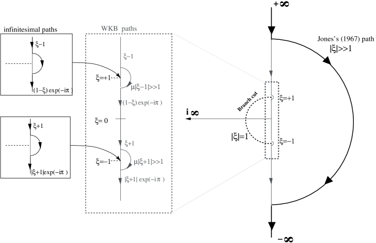
Figure 1: Paths used for the integration of the vertical structure equation (2.4); see also Figure 1 in Jones (1967) and note that our real $\xi$-axis is vertical while Jones’s is horizontal.

After involved manipulations it can be shown that the reflection and transmission coefficients are given by

$$R=\frac{C}{D}=0\quad\hbox{and}\quad T=\frac{1}{D}=i\mathrm{e}^{-\mu\pi},$$ (2.12)

where $\mu^{2}=J(1+\nu^{2})-1/4$ (see Appendix A.1). This is the result of Jones (1967), which can be obtained much more directly by integration along a semi-circle with $|\xi|\gg 1$, as recalled in the introduction (see Fig. 1). Our solution provides the details of the solution between the inertial levels that this result ignores. In particular, it makes it possible to compute the EP flux, proportional to

$$F^{z}=\mathrm{Re}\,\left(i\frac{1-\xi^{2}}{\xi^{2}}W_{\xi}W^{*}-\nu\frac{WW^{*}}{\xi^{2}}\right),$$ (2.13)

and constant apart from jumps at the inertial levels (this conservation law is derived directly from (2.4) by multiplying by $W^{*}$ and integrating by parts). We can obtain the three distinct values of the EP flux on either side of and between the inertial levels using the first terms in the expansion of the hypergeometric functions for $\xi\to\pm\infty$ and $\xi\to 0$. Computations detailed in the Appendix show that the ratios of the EP flux between and above the inertial levels to the EP flux below are

$$\frac{F^{z(\mathrm{II})}}{|F^{z(\mathrm{I})}|}=\frac{\mathrm{e}^{2\pi\nu}+1}{\mathrm{e}^{2\pi\mu}-1}\quad\textrm{and}\quad\frac{F^{z(\mathrm{III})}}{|F^{z(\mathrm{I})}|}=\mathrm{e}^{-2\pi\mu},$$ (2.14)

where the absolute value in the denominators is required because the incoming EP flux $F^{z(\mathrm{I})}<0$ whereas the other two fluxes are positive (see Appendix). The first of these ratios describes the crossing of the lower inertial level by the incident waves and displays the strong dependence on the direction $\nu$ of the wavevector that characterises the valve effect. It is shown as a function of $\nu$ and $J$ in Fig. 2. The figure indicates that, for $J<1$, the ratio can exceed 1 and can take very large values for $\nu>0$. We discuss this phenomenon further in section 4.

Figure 2: Ratio of the EP flux between the inertial levels to the incident EP flux as a function of the Richardson number $J$ and wave aspect ratio $\nu=l/k$.

3 WKB approximation and tunnelling

A WKB solution of (2.4), strictly valid for $\mu\gg 1$ but qualitatively correct for $\mu\gtrsim 1$, sheds light on the behaviour of the solution and on the valve effect in particular. To derive this solution, it is convenient to follow Miyahara (1981) and recast (2.4) in the canonical form

$$\Psi_{\xi\xi}+\left[\frac{\mu^{2}+{1}/{4}}{\xi^{2}-1}+\frac{(3+\nu^{2})\xi^{2}-2}{\xi^{2}(\xi^{2}-1)^{2}}\right]\Psi=0,$$ (3.15a)

where

$$W(\xi)=\xi(\xi-1)^{-1/2+i\nu/2}\left(\xi+1\right)^{-1/2-i\nu/2}\Psi(\xi).$$ (3.15b)

Assuming $\mu\gg 1$, we then introduce the expansion

$$\Psi(\xi)=\left(\Psi_{0}(\xi)+\mu^{-1}\Psi_{1}(\xi)+...\right)\mathrm{e}^{\mu\int^{\xi}\phi(\xi^{\prime})d\xi^{\prime}}$$ (3.16)

and find at orders $\mu^{2}$, $\mu$ and $1$ that

$$\phi=\frac{\epsilon i}{\sqrt{\xi^{2}-1}},\ \ \Psi_{0}=\left(\xi^{2}-1\right)^{1/4}\ \ \textrm{and}\ \ \Psi_{1}=-\epsilon i\frac{1+(\nu^{2}/2-7/8)\xi^{2}}{\xi(\xi^{2}-1)^{1/4}},$$ (3.17)

where $\epsilon=\pm 1$ selects the two possible solutions. The expansion (3.16) breaks down in the regions $||\xi|-1|=O(\mu^{-2})$ surrounding the inertial levels where an approximation in terms of Hankel functions can be constructed (see LPV12 for the rescaling leading to this conclusion). Here we avoid this complication by integrating (3.15a) along a path that remains at a distance larger than $\mu^{-1}$ from the inertial levels and avoids the branch cut (see Fig. 1). This path does not cross the only Stokes line (where $\operatorname{Im}\phi=0$, e.g., Ablowitz & Fokas 1997), namely $\xi\in[-1,1]$. Therefore, a single WKB solution, determined by the radiation condition to correspond to $\epsilon=1$, can be continued from $\xi\to\infty$ to $\xi\to-\infty$. To make the absorptive properties more transparent, we express the approximations at order $\mu$ for a unit-amplitude incident wave (rather than for a unit-amplitude transmitted wave in the exact case, see Appendix A.3 for details). This gives

$$\begin{array}[]{lcrccr}W_{\mathrm{WKB}}^{(\mathrm{III})}=&&-ig(\xi)&\mathrm{e}^{-\mu\pi}&\mathrm{e}^{i\mu\ln\left(\xi+\sqrt{\xi^{2}-1}\right)}&\,\mbox{for}\;\xi>1,\end{array}$$ (3.18a)

$$\begin{array}[]{lcrccr}W_{\mathrm{WKB}}^{(\mathrm{II})}=&-\mathrm{e}^{\nu\pi/2}&\frac{1-i}{\sqrt{2}}g(\xi)&&\mathrm{e}^{-\mu(\pi/2+\sin^{-1}\xi)}&\;\mbox{for}\;-1<\xi<1,\end{array}$$ (3.18b)

$$\begin{array}[]{lcrccr}W_{\mathrm{WKB}}^{(\mathrm{I})}=&&g(\xi)&&\mathrm{e}^{i\mu\ln\left(|\xi|+\sqrt{\xi^{2}-1}\right)}&\mbox{for}\;\xi<-1.\end{array}$$ (3.18c)

Here, the function $g(\xi)=\xi|\xi-1|^{-\frac{1}{4}+i\frac{\nu}{2}}|\xi+1|^{-\frac{1}{4}-i\frac{\nu}{2}}$ groups the factors unaffected by the absorptive properties of the shear layer; because it is expressed in terms of absolute values of $\xi\pm 1$, the complex powers $-1/4\pm i\nu/2$ apply to purely positive real arguments, and the effect of the continuations (2.9) appears explicitly through exponential factors in (3.18a)–(3.18b). Note that for $|\xi|\gg 1$, $\mathrm{e}^{i\mu\ln\left(|\xi|+\sqrt{\xi^{2}-1}\right)}\approx 2^{i\mu}|\xi|^{i\mu}$ and $g(\xi)\approx\mbox{sign}(\xi)|\xi|^{1/2}$, so $W_{\mathrm{WKB}}^{(\mathrm{I})}=|\xi|^{1/2+i\mu}$, recovering the incident wave in (2.8) (up to an irrelevant phase factor).

The WKB solution (3.18) is instructive in several respects. First, as $\xi\to\pm\infty$, it reproduces exactly the ratio between the amplitudes of the upward-propagating IGWs (2.7) and (2.8) found from the exact solution. In particular, the reflection and transmission coefficients are the exact ones in (2.12). The WKB solution also shows that the amplitude of the solution is dominated by the exponential term $\mathrm{e}^{-\mu\sin^{-1}\xi}$ in (3.18b) that rapidly decays monotonically between the inertial levels. This decay is strongly reminiscent of the exponential decay that characterizes the neutral solution in the quasi-geostrophic approximation. This can be made more transparent by noting that near the critical level $\xi=0$, the $O(\mu^{-1})$ term (retaining $\Psi_{1}$ in (3.16)) is proportional to the quasi-geostrophic solution $\left(1+\mu\xi\right)\mathrm{e}^{-\mu\xi}$ (see Eq. (2.16) in LPV12). Away from the immediate vicinity of $\xi=0$, the decay is in fact faster than predicted by the quasi-geostrophic approximation since $|\sin^{-1}\xi|\geq\xi$. The valve effect is also evident in the WKB solution, through the factor $\hbox{e}^{\nu\pi/2}$ in (3.18b). The dependence of the amplitude on $\nu$ associated to this factor is however weak compared to the dependence on $J$ and $|\nu|$ stemming from the factor $\mathrm{e}^{-\mu(\pi/2+\sin^{-1}\xi)}\sim\mathrm{e}^{-\sqrt{J(1+\nu^{2})}(\pi/2+\sin^{-1}\xi)}$ in (3.18b) since $J\gg 1$. This factor represents a very rapid amplitude decay of the solution above $\xi=-1$, and corresponds to an absorption that increases rapidly with $J$ and $|\nu|$: the asymmetry that favours perturbations with $\nu>0$ over those with $\nu<0$ between the inertial levels is of little significance compared to this absorption.

The WKB solution represents the exact solution accurately even for moderately large $J$. For $J=5$, for instance, the two solutions almost coincide everywhere except in regions close to the inertial levels (see Fig. 3). The WKB approximation deteriorates around the lower inertial level for $|\xi+1|\lesssim 0.05$ (see Fig. 3b), corresponding to an $O(\mu^{-1})$ distance to the inertial level, as expected. An analogous breakdown of the WKB approximation occurs for $\xi\approx 1$, but in this case the solutions are very small.

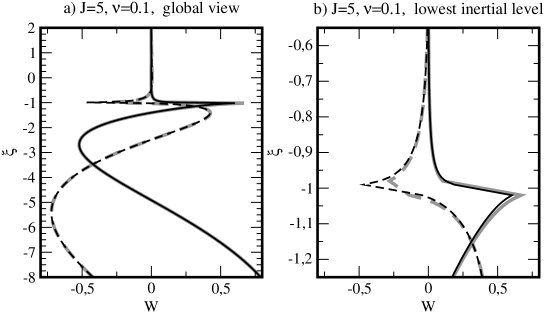
Figure 3: Vertical velocity $W$ for the exact solution (2.6a)-(2.6c) ($\mathrm{Re}\,W$, black solid; $\operatorname{Im}W$, black dashed) and the WKB approximation (3.18a)-(3.18c) ($\mathrm{Re}\,W_{\mbox{\tiny WKB}}$ grey solid and $\operatorname{Im}W_{\mbox{\tiny WKB}}$ grey dashed) for $J=5$, $\nu=0.1$: (a) global view; (b) zoom on the lowest inertial level.

Figure 3 also illustrates how the solution behaves as an upward-propagating wave – with real and imaginary parts in quadrature – outside the inertial levels (see Fig. 3a), and as an evanescent perturbation – with real and imaginary parts in phase – between the inertial levels (see Fig. 3b). This behaviour can be interpreted as a form of tunnelling, analogous to, but different from the classical tunnelling between turning points as described, for instance, by Bender and Orszag (1978). The continuity of the arguments of the last exponential factors in (3.18) shows that the amplitude decrease of the transmitted signal by the factor $\hbox{e}^{-\mu\pi}$ can be immediately related to the decay of the solution $W^{(\mathrm{II})}_{\tiny\mbox{WKB}}$ between the inertial level as $\mathrm{e}^{-\mu(\pi/2+\sin^{-1}\xi)}$ since this decreases by the same factor $\hbox{e}^{-\mu\pi}$. In the tunnelling interpretation, the valve effect seems to play no role, because the amplitude jump $\hbox{e}^{\nu\pi/2}$ through the lower inertial level is exactly balanced by the inverse jump $\hbox{e}^{-\nu\pi/2}$ at the upper inertial level.

An obvious difference with classical tunnelling is the absence of a fully conserved flux. In classical tunnelling, wave-action flux conservation leads to the relation $|T|^{2}+|R^{2}|=1$ that constrains the transmission and refection coefficients. Here, the analogous conservation is that of the EP flux, but because this can jump at the inertial level (Eliassen and Palm 1961, Grimshaw 1975), there is no associated constraint on $T$ and $R$, making the absence of reflection $R=0$ compatible with partial (indeed very weak) transmission $|T|<1$. Regarding the EP flux, we note that the WKB solution between the inertial levels (3.18b) suggests a zero flux, since it is evanescent (see for instance Gill 1982). The flux is non zero, however, and can be captured by extending the WKB analysis to take into account the Stokes phenomenon that arises at $\xi=1$. The relevant computation, carried out in LPV12, reveals the presence of an exponentially small solution increasing exponentially with $\xi$ to be added to (3.18b). Taking this into account gives a non-zero flux, deduced from Eq. (2.31) in LPV12 to satisfy

$$\frac{F^{z(\mathrm{II})}}{|F^{z(\mathrm{I})}|}\sim\mathrm{e}^{-2\pi\mu}(\mathrm{e}^{2\pi\nu}+1),$$ (3.19)

consistent with (2.14) for $\mu\gg 1$.

4 Valve effect and inertial instability

To describe further the valve effect, we return to the exact solutions and first present vertical profiles of $W$ when $J=5$ and for $\nu=\pm 1$ in Fig. 4 . The global views in Figs. 4a and 4c show that the solutions are almost identical. Even though a closer examination of the solution at the lowest inertial levels (Figs. 4b and 4d) shows that the solution with $\nu>0$ is amplified whereas that with $\nu<0$ is attenuated, this difference matters little because of the very rapid decay with $\xi$ of both solutions between the inertial levels. Also in Fig. 4, we see that the EP flux is very small between the inertial levels consistent with expression (2.14) for the ratio ${F^{z(\mathrm{II})}}/{|F^{z(\mathrm{I})}|}$ of the EP flux between the inertial level to the incident EP flux. For $J\gg 1$, this ratio is approximated by (3.19) which shows, as discussed, that the valve effect plays only a minor role in modulating it.

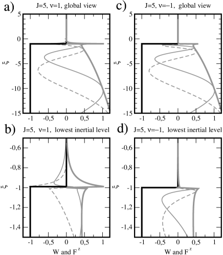
Figure 4: Vertical velocity $W$ for the exact solution (2.6a)-(2.6c) ($|W|$ thick grey solid, $\mathrm{Re}\,W$ grey solid, and $\operatorname{Im}W$ grey dashed) and EP flux $F^{z}$ from (2.13) (black solid) for $J=5$ and $\nu=\pm 1$. The EP flux is normalized by its incident value: (a) and (c) global views for $\nu=\pm 1$; (b) and (d) zooms on the lowest inertial level.

For $J<1$, the situation is different, and the valve effect can lead to an intensification of the perturbation between the inertial levels. This is illustrated in Figure 5 which shows profiles of $W$ and $F^{z}$ for $J=0.5$ and $\nu=\pm 2$. When $\nu=2$ in Figs. 5a-b, the incident wave is clearly amplified as it passes through the lower inertial level (Fig. 5b), and the solution between the inertial levels does not display the almost exponential decay with altitude that characterizes the solution when $J\gg 1$. The behaviour for $\nu=-2$ illustrated in Figs. 5c-d is then completely different since the incident wave is almost entirely absorbed at the lowest inertial level. This pronounced difference between positive and negative $\nu$ translates in the EP fluxes ratios in (2.14) as Fig. 2 confirms. More importantly, (2.14) tells that the disturbance with $\nu>\sqrt{(J-1/4)/(1-J)}$ are amplified between the inertial levels when $J<1$ (in this case the ratio is larger than $1$). More than this, for $|\nu|\gg 1$,

$$\frac{F^{z(\mathrm{II})}}{|F^{z(\mathrm{I})}|}\sim\mathrm{e}^{2\pi(\nu-\sqrt{J}|\nu|)},$$ (4.20)

so the amplification is arbitrarily large for $\nu\to+\infty$ when $J<1$.

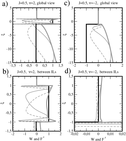
Figure 5: Same as Fig. 4 but for $J=0.5$, $\nu=\pm 2$. In a) and b), the EP flux is normalized by its amplitude between the inertial layers. Note the change of scale in panel (d).

It is interesting to relate this result to inertial instability, which also occurs when $J<1$ (Stone 1966), a condition that implies that the background flow potential vorticity is negative (Bennetts and Hoskins 1979). Inertial instability – or symmetric instability – arises for perturbations with $k=0$, that is, $\nu=\infty$, a case that we have not treated explicitly. It is examined in Stone (1966) and can be recovered easily by replacing the non-dimensional variable $\xi$ defined in (2.5) and clearly inappropriate for $k=0$ by the original $z$. This reduces the equation for $W$ to

$$\left(f^{2}-\omega^{2}\right)W_{zz}+2i\Lambda flW_{z}-J\Lambda^{2}l^{2}W=0$$ (4.21)

which admits the simple solution $W\propto\exp(imz)$ for

$$\omega^{2}=f^{2}\left(J\delta^{2}+2\delta+1\right),$$ (4.22)

where $\delta=(\Lambda l)/(fm)$. A purely imaginary frequency $\omega$, corresponding to symmetric instability, occurs for $J<1$, with maximum growth rate $\mathrm{Im}\,\omega=f\sqrt{1/J-1}$ for $\delta=-1/J$.

Although our analysis is not adapted to treat this case, because when $k\rightarrow 0$ the inertial levels go to infinity and it becomes impossible to impose radiation conditions beyond them, the condition $J<1$ for IGW amplification between the inertial levels establishes a clear connection between the valve effect and the inertial instability criteria. This connection with inertial instability is not the only one. For instance, the fact that waves with large $\nu$ are amplified between the inertial levels suggests that the shear layer response to a random incident IGW field can become very large between the inertial levels and preferentially symmetric as are inertial instabilities. Also, the response in this transverse plane will be tilted in the direction of the isentropes (see Figs. 2d and 2h in LPV12) as is also the case for inertial instability since $\delta<0$ for them (see (4.22)). Note also that a stabilization of the flow by the disturbance is expected to occur in the nonlinear regime. Indeed the large increase of the EP flux at the lower inertial level accelerates the mean flow there, whereas the decrease at the upper inertial level decelerates it there. As a result, the positive shear tends to be reduced: as is often the case, the development of the instability weakens its cause.

5 Conclusion

The problem of the absorptive properties of gravity waves by critical levels analyzed by Booker and Bretherton (1967) is one of the cornerstone of dynamical meteorology. Its extension to the rotating case, even in the simple set-up with constant shear, constant stratification and without boundaries has been therefore studied by many investigators. Nevertheless, as the mathematics are involved, its exact solution has never been given adequately over the full domain. This paper gives this solution and interprets it, partly using a WKB approximation.

In the general case, the structure of the solution is as follows. A monochromatic wave incident at the lower inertial level (there is no reflected wave) is amplified or attenuated by the valve effect, depending on the Richardson number and on the orientation of the wavevector. Between the inertial levels the disturbance consists of two independent solutions (2.6b); in the WKB as in the QG approximation, these two solutions are necessary to explain a non-zero EP flux. The amplification (attenuation) at the lower inertial level is compensated by an inverse attenuation (amplification) at the upper inertial level, so that the overall attenuation between the two inertial levels is controlled by the decrease of the solution across the region in a manner akin to quantum tunnelling. The analogy is not complete, however, in particular because there is no reflected gravity wave.

The situation is particularly transparent for large Richardson number $J\gg 1$, when a WKB approximation provides the solution in terms of elementary functions. In this case, the solution between the inertial levels is dominated by an exponentially decaying part, analogous to that predicted in the QG approximation. An exponentially small, exponentially growing solution is however present and ensures the constancy of the EP flux; this solution can be derived by careful consideration of the Stokes phenomenon (see LPV12 for details).

When $J$ is smaller, the decay of the balanced solution with altitude is not as pronounced, and the valve effect becomes significant, leading to a strong dependence of the wave amplitude between the inertial levels on the wavevector orientation. For $J<1$, in particular, waves with large $\nu$, experience an amplification, with an EP flux between the inertial levels that is larger than that of the incident wave. This establishes a connection between the absorptive properties of the inertial levels and the criterion $J<1$ for inertial (symmetric) instability. This connection is not apparent either in the classical transmission coefficient in (1.1) or in the formula for the valve effect in (1.2). Practically, this demonstrates how small non-symmetric disturbances can become very large in inertially unstable flow, providing there is a small external excitation.

Acknowledgments. This work was supported by the European Commission’s 7th Framework Programme, under the projects EMBRACE (Grant agreement 282672), and by the French ANR project StradyVarius. The authors acknowledge the International Space Science Institude in Bern for hosting two workshops about atmospheric gravity waves. We would also like to thank the three anonymous reviewers for their useful comments.

Appendix A Derivation details

A.1 Exact Derivation of $R$ and $T$

Following LPV12, the $W$ functions in (2.6a)-(2.6c) can be expressed in terms of hypergeometric functions $F$. Using Eqs. (15.5.3), (15.5.4), (15.5.6) and (15.5.7) in Abramowitz and Stegun (1964) (hereafter AS), we write

$$W_{u}^{(\mathrm{III})}=(1+\xi)^{-i\nu}\xi^{-2b}F(a^{\prime},b^{\prime};c^{\prime};\xi^{-2}),$$ (A.23a)

$$W_{d}^{(\mathrm{II})}=(1+\xi)^{-i\nu}F(a,b;c;\xi^{2}),\;W_{u}^{(\mathrm{II})}=(1+\xi)^{-i\nu}\xi^{3}\,F(a^{\prime\prime},b^{\prime\prime};c^{\prime\prime};\xi^{2}),$$ (A.23b)

$$W_{d}^{(\mathrm{I})}=\left(|\xi|-1\right)^{-i\nu}|\xi|^{-2a}F(a^{\prime\prime\prime},b^{\prime\prime\prime};c^{\prime\prime\prime};|\xi|^{-2}),W_{u}^{(\mathrm{I})}=\left(|\xi|-1\right)^{-i\nu}|\xi|^{-2b}F(a^{\prime},b^{\prime};c^{\prime};|\xi|^{-2})$$ (A.23c)

In these expressions, the coefficients $a$, $b$ and $c$ are given by

$$a=-\frac{1}{4}-i\frac{\nu-\mu}{2},\quad b=-\frac{1}{4}-i\frac{\nu+\mu}{2},\quad c=-\frac{1}{2},$$ (A.24)

and $\mu=\sqrt{J(1+\nu^{2})-1/4}$. The other coefficients are linear combinations of $a$, $b$ and $c$: $a^{\prime}=b$, $b^{\prime}=b-c+1$, $c^{\prime}=b-a+1$, $a^{\prime\prime}=a-c+1$, $b^{\prime\prime}=b-c+1$, $c^{\prime\prime}=2-c$, $a^{\prime\prime\prime}=a$, $b^{\prime\prime\prime}=a-c+1$ and $c^{\prime\prime\prime}=a-b+1$. Then to evaluate the complex constants $A$, $B$, $C$ and $D$ we match (2.6a) and (2.6b) in the vicinity of $\xi=1$ and (2.6b) and (2.6c) in the vicinity of $\xi=-1$ along the contour displayed in Fig. 1 (see also Eq. (2.9)). Using (A.23a)– (A.23c) and the transformation formula (15.3.6) in AS, we obtain

$$W\sim\alpha^{\prime}(\xi-1)^{i\nu}+2^{-i\nu}\beta^{\prime}\quad\textrm{as}\,\ \xi\to 1^{+},$$ (A.25a)

$$W\sim\left(\alpha A+\alpha^{\prime\prime}B\right)(1-\xi)^{i\nu}+2^{-i\nu}(\beta A+\beta^{\prime\prime}B)\quad\textrm{as}\,\ \xi\to 1^{-},$$ (A.25b)

$$W\sim 2^{i\nu}(A\alpha-B\alpha^{\prime\prime})+\left(1+\xi\right)^{-i\nu}\left(A\beta-B\beta^{\prime\prime}\right)\,\ \xi\to-1^{+},$$ (A.25c)

$$W\sim 2^{i\nu}(C\alpha^{\prime\prime\prime}+D\alpha^{\prime})+\left(|\xi|-1\right)^{-i\nu}\left(C\beta^{\prime\prime\prime}+D\beta^{\prime}\right)\,\ \xi\to-1^{-}.$$ (A.25d)

In these expressions the $\alpha$’s and the $\beta$’s are related to the $a,b,c$’s by

$$\alpha=\frac{\Gamma(c)\Gamma(a+b-c)}{\Gamma(a)\Gamma(b)}\quad\textrm{and}\quad\beta=\frac{\Gamma(c)\Gamma(c-a-b)}{\Gamma(c-a)\Gamma(c-b)},$$ (A.26)

where $\Gamma$ is the gamma function (see AS, chapter 6). As a first step to determine $A$, $B$, $C$ and $D$ it should be noticed that the 8 coefficients $\alpha$’s and $\beta$’s can ultimately be expressed in terms of the 4 coefficients $\alpha$, $\alpha^{\prime}$, $\beta^{\prime}$, and $\alpha^{\prime\prime}$, given explicitly as

$${\color[rgb]{0,0,0}\alpha^{\prime}=\frac{\Gamma(1-i\mu)\Gamma(-i\nu)}{\Gamma(b)\Gamma(1-b^{*})},\quad\beta^{\prime}=\frac{\Gamma(1-i\mu)\Gamma(i\nu)}{\Gamma(1-a)\Gamma(a^{*})},}$$ (A.27a)

$${\color[rgb]{0,0,0}\alpha=\frac{-2\sqrt{\pi}\Gamma(-i\nu)}{\Gamma(a)\Gamma(b)},\quad\alpha^{\prime\prime}=\frac{3\sqrt{\pi}\Gamma(-i\nu)}{4\Gamma(1-a^{*})\Gamma(1-b^{*})},}$$ (A.27b)

through the relations $\beta=\alpha^{*}$, $\beta^{\prime\prime}=\alpha^{\prime\prime*}$, $\alpha^{\prime\prime\prime}=\beta^{\prime*}$ and $\beta^{\prime\prime\prime}=\alpha^{\prime*}$.

Requiring that the continuations match (A.25b) and (A.25d) determines the constants $A$, $B$ and $C$, $D$ through Matching near $\xi=1$ and $\xi=-1$ yields the linear systems (2.10)–(2.11). Solving (2.10) for $A$ and $B$ gives

$${\color[rgb]{0,0,0}A=\frac{\alpha^{\prime\prime}\beta^{\prime}}{\delta_{1}}-\frac{\alpha^{\prime\prime*}\alpha^{\prime}}{\delta_{1}}\hbox{e}^{\pi\nu},}$$ (A.28a)

$${\color[rgb]{0,0,0}B=\frac{\alpha^{\prime}\alpha^{*}}{\delta_{1}}\hbox{e}^{\pi\nu}-\frac{\alpha\beta^{\prime}}{\delta_{1}}.}$$ (A.28b)

Solving (2.11) for $C$ and $D$ gives

$${\color[rgb]{0,0,0}C=\frac{\beta^{\prime}(A\alpha-B\alpha^{\prime\prime})}{\delta_{2}}-\frac{\alpha^{\prime}(A\alpha^{*}-B\alpha^{\prime\prime*})}{\delta_{2}}\hbox{e}^{-\pi\nu},}$$ (A.29a)

$${\color[rgb]{0,0,0}D=\frac{\beta^{\prime*}(A\alpha^{*}-B\alpha^{\prime\prime*})}{\delta_{2}}\hbox{e}^{-\pi\nu}-\frac{\alpha^{\prime*}(A\alpha-B\alpha^{\prime\prime})}{\delta_{2}}.}$$ (A.29b)

In these equations, $\delta_{1}$ and $\delta_{2}$ are determinants appearing in (2.10)–(2.11), explicitly given by

$${\color[rgb]{0,0,0}\delta_{1}=\alpha^{*}\alpha^{\prime\prime}-\alpha\alpha^{\prime\prime*}\quad\hbox{and}\quad\delta_{2}=|\beta^{\prime}|^{2}-|\alpha^{\prime}|^{2}.}$$ (A.30)

A closer examination of (A.27)–(A.29) shows that the Gamma functions involved appear through products expressible in terms of ordinary trigonometric functions using the reflection formula

$$\Gamma(z)\Gamma(1-z)=\frac{\pi}{\sin\pi z}$$ (A.31)

and the two related formulas (6.1.29) and (6.1.31) in AS. We now sketch the necessary calculation. For brevity we introduce the notation $s=\sin(\pi a^{*})$ and $t=\sin(\pi b)$. Applying (A.31) with $z=a^{*}$ and $z=b$ thus reduces the right-hand sides to $\pi s^{-1}$ and $\pi t^{-1}$, respectively.

Substituting (A.27) into the two equations in (A.30) gives

$${\color[rgb]{0,0,0}\delta_{1}=\frac{3}{2}\frac{ts^{*}-st^{*}}{\nu\sinh(\pi\nu)}\quad\hbox{and}\quad\delta_{2}=\frac{\mu}{\nu}\frac{|s|^{2}-|t|^{2}}{\sinh(\pi\nu)\sinh(\pi\mu)}.}$$ (A.32)

These equations can be further simplified using common trigonometric identities and the definitions of $a$, $b$ and $c$ in terms of $\nu$ and $\mu$. A direct calculation gives

$${\color[rgb]{0,0,0}ts^{*}-st^{*}=i\sinh(\pi\nu)\quad\hbox{and}\quad|s|^{2}-|t|^{2}=-\sinh(\pi\mu)\sinh(\pi\nu),}$$ (A.33)

reducing the determinants to

$${\color[rgb]{0,0,0}\delta_{1}=\frac{3i}{2\nu}\quad\hbox{and}\quad\delta_{2}=-\frac{\mu}{\nu}.}$$ (A.34)

We can use this approach to obtain exact formulas for the transmission and reflection coefficients. These coefficients are defined by $T=D^{-1}$ and $R=CD^{-1}$, which requires the calculation of $C$ and $D$. Substituting (A.28a) and (A.28b) into (A.29b) gives

$$D=\frac{2\hbox{Re}(\alpha\alpha^{\prime\prime*})(|\beta^{\prime}|^{2}\hbox{e}^{-\pi\nu}+|\alpha^{\prime}|^{2}\hbox{e}^{\pi\nu})-4\hbox{Re}(\alpha\alpha^{\prime\prime}\beta^{\prime}\alpha^{\prime*})}{\delta_{1}\delta_{2}},$$ (A.35)

where the functions involving the constants $\alpha^{\prime}$, $\beta^{\prime}$, $\alpha$ and $\alpha^{\prime\prime}$ in the numerator can be expressed in terms of $s$ and $t$ as

$$\alpha^{*}\alpha^{\prime\prime}=\delta_{1}\frac{st^{*}}{st^{*}-ts^{*}},$$ (A.36a)

$$\alpha\alpha^{\prime\prime}\beta^{\prime}\alpha^{\prime*}=-\delta_{1}\delta_{2}\frac{|s|^{2}|t|^{2}}{(|s|^{2}-|t|^{2})(ts^{*}-st^{*})},$$ (A.36b)

$$|\alpha^{\prime}|^{2}=\delta_{2}\frac{|t|^{2}}{|s|^{2}-|t|^{2}}\quad\hbox{and}\quad|\beta^{\prime}|^{2}=\delta_{2}\frac{|s|^{2}}{|s|^{2}-|t|^{2}}.$$ (A.36c)

Substituting (A.36) into (A.35), we note that the factor $\delta_{1}\delta_{2}$ appears in both the numerator and the denominator. Using trigonometric identities, we finally obtain the simple form

$$D=-i\mathrm{e}^{\pi\mu},$$ (A.37)

or equivalently, $T=D^{-1}=i\mathrm{e}^{-\pi\mu}$.

The derivation of a formula for the reflection coefficient follows the same argument. An expression for $C$ is obtained by substituting (A.28) into (A.29a), and the product of coefficients $\alpha^{\prime}$, $\beta^{\prime}$, $\alpha^{\prime\prime}$ is expressed in terms of the trigonometric functions $s$ and $t$, using the reflection formula. Hence, we deduce

$$C=2\delta_{1}^{-1}\delta_{2}^{-1}\left[\alpha\alpha^{\prime\prime}\beta^{\prime 2}+(\alpha\alpha^{\prime\prime})^{*}\alpha^{\prime 2}-2\alpha^{\prime}\beta^{\prime}\cosh(\pi\nu)\hbox{Re}(\alpha^{*}\alpha^{\prime\prime})\right].$$ (A.38)

along with the two relations

$$\alpha\alpha^{\prime\prime}\beta^{\prime 2}+\alpha^{\prime 2}(\alpha\alpha^{\prime\prime})^{*}=-\frac{2\pi}{3}\delta_{1}^{2}\frac{\Gamma^{2}(1-i\mu)}{P(a,b)}\frac{|s|^{2}+|t|^{2}}{(ts^{*}-st^{*})^{2}},$$ (A.39a)

$$2\alpha^{\prime}\beta^{\prime}\hbox{Re}(\alpha^{*}\alpha^{\prime\prime})=-\frac{2\pi}{3}\delta_{1}^{2}\frac{\Gamma^{2}(1-i\mu)}{P(a,b)}\frac{st^{*}+s^{*}t}{(ts^{*}-st^{*})^{2}},$$ (A.39b)

where $P(a,b)=\Gamma(a^{*})\Gamma(b)\Gamma(1-b^{*})\Gamma(1-a)$. After some direct algebra, we find

$$C=0,$$ (A.40)

or equivalently, $R=0$, which is valid to all orders in $\mu$.

A.2 EP flux jump between the inertial levels

From (2.6b), (A.23b), and the definition of the Gauss hypergeometric series (15.1.1 in AS), we can show that near $\xi=0$

$$W=A\left(1-i\nu\xi-\left(\frac{\mu^{2}}{2}+\frac{1}{8}\right)\xi^{2}-i\nu\left(\frac{\nu^{2}}{3}-\frac{\mu^{2}}{2}+\frac{5}{24}\right)\xi^{3}\right)+B\xi^{3}+O(\xi^{4}).$$ (A.41)

From $F^{z}$ evaluated very near $\xi=0$ using (2.13), we deduce that $F^{z}=F^{z(\mathrm{II})}={3i}\left(BA^{*}-AB^{*}\right)/2$ between the inertial levels. Similarly, using the asymptotics form for $W$ as $\xi\to-\infty$, we deduce that $F^{z(I)}=-\mu DD^{*}$ below $\xi=-1$. The ratio of the EP flux between the inertial levels to the incident EP flux is therefore given by

$$\frac{F^{z(\mathrm{II})}}{|F^{z(\mathrm{I})}|}=\frac{3i}{2\mu}\frac{BA^{*}-AB^{*}}{DD^{*}}.$$ (A.42)

According to (A.37), the denominator of (A.42) can be simplified to $DD^{*}=\hbox{e}^{2\mu\pi}$, while the numerator takes a more complicated form. Using (A.28), we obtain

$$BA^{*}-AB^{*}=\frac{1}{|\delta_{1}|^{2}}\left(\hbox{e}^{2\pi\nu}|\alpha^{\prime}|^{2}-|\beta^{\prime}|^{2}\right)\left(\alpha\alpha^{\prime\prime*}-\alpha^{*}\alpha^{\prime\prime}\right).$$ (A.43)

Upon substituting (A.36a) and (A.36c) into (A.43), we obtain

$$BA^{*}-AB^{*}=-\frac{2\mu}{3}\frac{(s^{*}t-st^{*})(\hbox{e}^{2\pi\nu}|t|^{2}-|s|^{2})}{\sinh^{2}(\pi\nu)\sinh(\pi\mu)}.$$ (A.44)

This equation can be further simplified using (A.33) and the identity

$$\hbox{e}^{2\pi\nu}|t|^{2}-|s|^{2}=\frac{1}{2}\hbox{e}^{\pi(\nu+\mu)}\sinh(2\pi\nu).$$ (A.45)

Using this, (A.42) reduces to

$$\frac{F^{z(\mathrm{II})}}{|F^{z(\mathrm{I})}|}=\frac{\cosh(\pi\nu)}{\sinh(\pi\mu)}\hbox{e}^{\pi(\nu-\mu)}=\frac{\hbox{e}^{2\pi\nu}+1}{\hbox{e}^{2\pi\mu}-1}.$$ (A.46)

A.3 Continuation of the WKB solution

At the order $\mu$, substitution of the WKB solutions (3.17) into expression (3.15b) for $W(\xi)$ when $\xi>1$ gives

$$W^{(\mathrm{III})}(\xi)=\xi(\xi-1)^{-1/4+i\nu/2}(\xi+1)^{-1/4-i\nu/2}\mathrm{e}^{i\mu\cosh^{-1}\xi},$$ (A.47)

where $\cosh^{-1}\xi=\ln\left(\xi+\sqrt{\xi^{2}-1}\right)$. To continue this solution below $\xi=1$, we write $(\xi-1)=(1-\xi)\mathrm{e}^{-i\pi}$ so $\cosh^{-1}\xi$ becomes $\ln\left(\xi-i\sqrt{1-\xi^{2}}\right)=i\sin^{-1}\xi-i{\pi}/{2}$. Therefore the continuation of $W^{(\mathrm{III})}$ reads

$$W^{(\mathrm{II})}(\xi)=\xi(1-\xi)^{-1/4+i\nu/2}\mathrm{e}^{\nu\pi/2+i\pi/4}(\xi+1)^{-1/4-i\nu/2}\mathrm{e}^{+\mu\pi/2-\mu\sin^{-1}\xi}.$$ (A.48)

To continue this function below $\xi=-1$, we write $\xi+1=|\xi+1|\mathrm{e}^{-i\pi}$ (and also $\xi=-|\xi|$), so $\sin^{-1}\xi$ transforms into $-i\ln\left(|\xi|+\sqrt{\xi^{2}-1}\right)-\pi/2$, leading to the continuation

$$W^{(\mathrm{I})}(\xi)=-\xi(1-\xi)^{-1/4+i\nu/2}\mathrm{e}^{-i\pi/2}|\xi+1|^{-1/4-i\nu/2}\mathrm{e}^{+\mu\pi+i\mu\ln\left(|\xi|+\sqrt{\xi^{2}-1}\right)}.$$ (A.49)

The solutions in (3.18a)–(3.18c) are just (A.47)–(A.49) multiplied by $i\mathrm{e}^{-\mu\pi}$ so that the incident wave has a unit amplitude.

References

Ablowitz M.J. and Fokas A.S., 1997 Complex variables: introduction and applications, Cambridge University Press.

Abramowitz M. and I.A. Stegun, 1964 Handbook of mathematical functions (9th edition), Dover Publications Inc., New York, 1045pp.

Alford, M.H., 2003, Redistribution of energy available for ocean mixing by long-range propagation of internal waves, Nature, 423, 159-162.

Andrews, D.G., J.R. Holton and C. B. Leovy, 1987, Middle atmosphere dynamics, Academic Press Inc. (London) LTD, 489p.

Bender, C.M., and S.A. Orszag, 1978 Advanced mathematical methods for scientists and engineers, McGraw-Hill int. book comp., 593pp.

Bennetts, D.A., and B.J. Hoskins, 1979 Conditional symmetric instability - a possible explanation for frontal rainbands, Quart. J. Roy. Met. Soc., 105, 945–962.

Booker, J.R. and F.P. Bretherton, 1967 The critical layer for internal gravity waves in a shear flow, J. Fluid Mech., 27, 513–539.

Eliassen, A. and E. Palm, 1961 On the transfer of energy in stationary mountain waves, Geofys. Publ., 22, 1–23.

Ferrari, R., and C. Wunsch, 2009 Ocean circulation kinetic energy: Reservoirs, sources and sinks, Annu. Rev. Fluid. Mech, 41, 253–282.

Gill, A., 1982 Atmosphere-Ocean Dynamics, Academic Press, 662p

Grimshaw, R, 1975 Internal gravity waves: critical layer absorption in a rotating fluid, J. Fluid Mech., 70, 287–304.

Gula, J. and V. Zeitlin, 2010 Instabilities of buoyancy driven coastal currents and their nonlinear evolution in the two-layer rotating shallow water model. Part I: Passive lower layer, J. Fluid Mech., 659, 69–93.

Hertzog, A., G. Boccara, R.A. Vincent, F. Vial, and P. Cocquerez, 2008 Estimation of gravity wave momentum flux and phase speeds from quasi-Lagrangian stratospheric balloon flights. Part II: Results from the Vorcore campaign in Antarctica, J. Atmos. Sci., 65, 3056–3070.

Howard, L.H., 1961 Note on a paper of John W. Miles, J. Fluid. Mech, 10, 509-512.

Inverarity, G.W. and G.J. Shutts, 2000 A general, linearized vertical structure equation for the vertical velocity: Properties, scalings and special cases, Quart. J. Roy. Meteor. Soc., 126, 2709–2724.

Jones, W.L., 1967 Propagation of internal gravity waves in fluids with shear flow and rotation, J. Fluid Mech., 30, 439–448.

Lindzen, R.S., 1988 Instability of plane parallel shear-flow (toward a mechanistic picture of how it works), Pure Applied Geophys., 126, 103–121.

Lott, F., H. Kelder, and H. Teitelbaum, 1992 A transition from Kelvin-Helmholtz instabilities to propagating wave instabilities, Phys. Fluids, 4, 1990–1997.

Lott, F., 1997 The transient emission of propagating gravity waves by a stably stratified shear layer, Quart. J. Roy. Meteor. Soc., 123, 1603–1619.

Lott, F., 2003 Large-scale flow response to short gravity waves breaking in a rotating shear flow, J. Atmos. Sci., 60, 1691–1704.

Lott F., R. Plougonven, and J. Vanneste, 2010 Gravity waves generated by sheared potential-vorticity anomalies, J. Atmos. Sci., 67, 157–170.

Lott, F., R. Plougonven, and J. Vanneste, 2012: Gravity waves generated by sheared three dimensional potential vorticity anomalies, J. Atmos. Sci., 69, 2134–-2151

Mamatsashvili, G.R., V.S. Avsarkisov, G.D. Chagelishvili, R.G. Chanishvili,and M. V. Kalashnik, 2010 Transient dynamics of nonsymmetric perturbations versus symmetric instability in baroclinic zonal shear flows, J. Atmos. Sci., 67, 2972–2989.

Marshall, J., and Coauthors, 2009 The CLIMODE field campaign: Observing the cycle of convection and restratification over the Gulf Stream. Bull. Amer. Meteor. Soc., 90, 1337–1350.

McWilliams J.C., 2003 Diagnostic force balance and its limits, in Nonlinear Processes in Geophysical Fluid Dynamics, Kluwer, ed: O. U. Velasco Fuentes, J. Sheinbaum and J. Ochoa, 287–304.

Miles, J.W., 1961: On the stability of heterogeneous shear flows, J. Fluid. Mech, 10, 496–508.

Miyahara, S., 1981 A note on the behavior of waves around the inertio frequency, J. Met. Soc. Japan, 59, 902–905.

Molemaker, M.J., J. C. McWilliams, and I. Yavneh, 2005, Baroclinic instability and loss of balance, J. Phys. Ocean., 35, 1505–1517.

Plougonven, R., and C. Snyder, 2007 Inertia-gravity waves spontaneously generated by jets and fronts. Part I: Different baroclinic life cycles, J. Atmos. Sci., 64, 2502–2520.

Plougonven, R., D.J. Muraki, and C. Snyder, 2005 A baroclinic instability that couples balanced motions and gravity waves, J. Atmos. Sci., 62, 1545–1559.

Rabinovitch, A., O.M. Umurhan, N. Harnik, F. Lott, and E. Heifetz 2011 Vorticity inversion and action-at-a-distance instability in stably stratified shear flow, J. Fluid Mech., 670, 301–325.

Richter, J.H., F. Sassi, and R.R. Garcia, 2010 Toward a physically based gravity wave source parameterization in a General Circulation Model, J. Atmos. Sci., 67, 136–156.

Sakai, S., 1989 Rossby–Kelvin instability: a new type of ageostrophic instability caused by a resonnance between Rossby waves and gravity waves, J. Fluid Mech., 202, 149–176.

Sato, K. and M. Yoshiki, 2008 Gravity wave generation around the polar vortex in the stratosphere revealed by 3-hourly radiosonde observations at Syowa station, J. Atmos. Sci., 65, 3719–3735.

Scavuzzo, C.M., M.A. Lamfri, H. Teitelbaum and F. Lott, 1998 A study of the low frequency inertio-gravity waves observed during PYREX, J. Geophys. Res., D2, 103, 1747–1758.

Shen, B.W., and Y.L. Lin, 1999 Effects of critical levels on two-dimensional back-sheared flow over an isolated mountain ridge on an f plane, J. Atmos. Sci., 56, 3286–3302.

Shutts G.J., 2003 Inertia–gravity wave and neutral Eady wave trains forced by directionally sheared flow over isolated hills, J. Atmos. Sci., 60, 593–606.

Stone, P.H., 1966 On non-geostrophic baroclinic instability, J. Atmos. Sci., 23, 390–400.

Sutyrin G.G., 2008 Lack of balance in continuously stratified rotating flows, J. Fluid Mech., 615, 93–100.

Vanneste J. and I. Yavneh, 2007 Unbalanced instabilities of rapidly rotating stratified sheared flows, J. Fluid Mech., 584, 373–396.

Whitt, D.B. and L.N. Thomas, 2013 Near-inertial waves in strongly baroclinic currents. J. Phys. Oceanogr., 43, 706–725.

Yamanaka, M. D., and H. Tanaka, 1984 Propagation and breakdown of internal inertia-gravity waves near critical levels in the middle atmosphere, J. Met. Soc. Japan, 62, 1–17.

Zuelicke, C. and D. Peters, 2008 Parameterization of strong stratospheric inertia-gravity waves forced by poleward-breaking Rossby waves, Month. Weath. Rev., 136, 98–119.