GASS: The Parkes Galactic All-Sky Survey.

Abstract

Context. The Galactic All-Sky Survey (GASS) is a survey of Galactic atomic hydrogen (H i) emission in the southern sky observed with the Parkes 64-m Radio Telescope. The first data release (GASS I) concerned survey goals and observing techniques, the second release (GASS II) focused on stray radiation and instrumental corrections.

Aims. We seek to remove the remaining instrumental effects and present a third data release.

Methods. We use the HEALPix tessellation concept to grid the data on the sphere. Individual telescope records are compared with averages on the nearest grid position for significant deviations. All averages are also decomposed into Gaussian components with the aim of segregating unacceptable solutions. Improved priors are used for an iterative baseline fitting and cleaning. In the last step we generate 3-D FITS data cubes and examine them for remaining problems.

Results. We have removed weak, but systematic baseline offsets with an improved baseline fitting algorithm. We have unraveled correlator failures that cause time dependent oscillations; errors are mostly proportional to the observed line intensity and cause stripes in the scanning direction. The remaining problems from radio frequency interference (RFI) are spotted. Classifying the severeness of instrumental errors for each individual telescope record (dump) allows us to exclude bad data from averages. We derive parameters that allow us to discard dumps without compromising the noise of the resulting data products too much. All steps are reiterated several times: in each case, we check the Gaussian parameters for remaining problems and inspect 3-D FITS data cubes visually. We find that in total $\sim 1.5$% of the telescope dumps need to be discarded in addition to $\sim 0.5$% of the spectral channels that were excluded in GASS II.

Conclusions. The new data release (GASS III) facilitates data products with improved quality. A new web interface, compatible with the previous version, is available for download of GASS III FITS cubes and spectra.

1 Introduction

The Parkes Galactic All-Sky Survey (GASS) maps the Galactic atomic hydrogen emission in the southern sky for declinations $\delta\la 1\degr$. The observations were made between January 2005 and October 2006 with the multibeam system on the 64-m Parkes Radio Telescope. McClure-Griffiths et al. (2009, Paper I) described the survey goals and observing techniques in detail. All of the initial data reduction and imaging for the first data release (GASS I) is also described in Paper I.

Observations of the Galactic H i  emission are affected by stray radiation received by the antenna diagram, and a correction is mandatory. The second data release (GASS II) was published after proper corrections became available (Kalberla et al. 2010, Paper II). At this stage it also turned out that part of the data was severely affected by radio frequency interference (RFI). About 0.5% of the data were discarded (see also Kalberla 2011) , but some RFI remained.

The GASS II RFI mitigation algorithm was based on median filtering, searching for sharp gradients in each individual observed spectrum. Spikes are typical for RFI but strong gradients can also have natural origin, such as absorption components and unresolved small scale fluctuations in the H i  distribution. This small scale structure can exist along filaments, and tests during the preparation of GASS II have shown that the applied median filtering could already degrade genuine emission features at low brightness temperatures $T_{B}\sim 2$ K. The RFI excision was therefore mostly restricted to channels with $T_{B}\la 0.5$ K, a very conservative approach with the aim of not impacting any genuine H i  emission features. Despite some remaining problems, priority was given to rapid publication.

Working with data products from GASS II revealed problems that made it desirable to improve the data processing in several respects:

1. Data may be affected by the remaining RFI, mostly in emission line regions with $T_{B}\ga 0.5$ K.

2. Maps can be degraded by stripes in the scanning direction, either right ascension or declination, predominantly in regions with strong H i  emission.

3. Baselines show occasional faint but systematic offsets, mostly along the borderline of the Galactic disk but also for isolated faint emission line features at high velocities.

4. Emission lines and instrumental baselines at positions with strong continuum emission are partly unreliable.

5. Some emission from local galaxies is badly treated by the baseline algorithm.

We decided to address these issues and, in the following, we present our investigations that led to a new data release (GASS III).

2 The iterative correction algorithm

2.1 General strategy

Dealing with instrumental problems is often a complex and difficult task. Individual strategies may fail to remove all problems in a single step. It is then necessary to iteratively repeat the approaches, step by step with an improved algorithm. This kind of strategy is, in case of the GASS, enforced by the fact that we are dealing with $2.8\,10^{7}$ spectral dumps for individual receivers and polarizations, each with 5 s integration time. This number does not allow for a visual inspection or correction of all individual dumps. Yet, the corrected data product needs to be inspected for remaining failures (The proof of the pudding is in eating, Cervantes 1615). We have done this in two ways, checking average H i  profiles and 3-D FITS cubes of the whole sky.

For a correction of instrumental problems our basic assumption is that only a fraction of the data is affected. The survey had two independent coverages, and therefore instrumental defects should mostly be spatially uncorrelated. Averaging these coverages should then diminish instrumental problems, in particular, if problematic data can be excluded from the average accordingly. Thus the first step of each iteration cycle is the generation of average profiles; our initial estimate was derived from GASS II. These averaged data can also be searched for remaining problems. We decompose all profiles into Gaussian components and check the results for outliers that might indicate instrumental problems.

To generate a new dump database, we use calibrated telescope data that have been corrected for stray radiation. These data are then corrected for instrumental baselines, as described in Paper II, except that we now use the previously determined average profiles to derive an initial estimates of the baseline fit. The data are then cleaned for RFI as described in Paper II. Each individual dump is compared with the nearest profile from the previously determined average, the rms deviation is recorded as a measure of the quality of the dump. Excluding bad data, we eventually generate 3-D FITS cubes for visual inspection, and we also proceed to calculate a new version of improved averages.

It is obvious that these iterations can only be successful if most of the data are of good quality and if other reliable criteria to define data as “good” or “bad” can be included without affecting features of the H i  brightness temperature distribution.

2.2 The HEALPix database

For a database containing average emission profiles, we would need to define a grid with constant distances to neighboring positions all over the sky. This scheme does not exist, but the Hierarchical Equal Area isoLatitude Pixelization (HEALPix, Górski et al. 2005) is a close approximation. HEALPix is a versatile structure for the pixelization of data on the sphere that also enables an easy comparison for data with different resolution. A single parameter, $N_{\mathrm{side}}$, defines the pixel resolution $\theta=\sqrt{3/\pi}\ 3600\hbox{${}^{\prime}$}/N_{\mathrm{side}}$ as well as the total number of pixels $N_{\mathrm{pix}}=12N_{\mathrm{side}}^{2}$ on the sphere. We have chosen $N_{\mathrm{side}}=1024$, corresponding to a resolution of $\theta=3\hbox{$.\mkern-4.0mu^{\prime}$}44,$ which is small in comparison to the average full width at half maximum (FWHM) GASS beamwidth of $14\hbox{$.\mkern-4.0mu^{\prime}$}4$. From the flagged dump database, we calculate all profiles on the HEALPix grid in each step of the iterations. Here we also include data available in the overlap regions for declinations $\delta\ga 1\degr$. For the GASS, the HEALPix database contains 6 655 155 profiles, 6 401 256 of these at $\delta\leq 1\degr$.

To generate the HEALPix database, we use a Gaussian convolution with a FWHM width of $7\hbox{$.\mkern-4.0mu^{\prime}$}5$ as the kernel. This results in an effective resolution of FWHM $16\hbox{$.\mkern-4.0mu^{\prime}$}2$ for the average spectra. The HEALPix database is updated every iteration cycle, excluding data that are affected by instrumental problems (see Sections 2.5 to 2.8). In the first step, we used the GASS II database.

When calculating the weighted arithmetic mean profile $T_{B}(v)$ on the HEALPix grid from $N$ available dumps, we take into account for each channel $j$ at the velocity $v_{j}$ that data may need to be excluded because of previous flagging, setting either $f_{i,j}=0$ or $f_{i,j}=1$. Here the index $i$ counts the observed dumps that are used for the average,

$$T_{B}(v_{j})=\frac{\sum_{i=1}^{N}w_{i}f_{i,j}T_{i}(v_{j})}{\sum_{i=1}^{N}w_{i}f_{i,j}}.$$ (1)

Here $w_{i}$ is the weight from the Gaussian kernel function. To trace the quality of individual averaged brightness temperature profiles we record the weights,

$$W(v_{j})=\sum_{i=1}^{N}w_{i}f_{i,j},$$ (2)

and the rms scatter $S(v_{j})$ from the unbiased weighted estimator

$$S^{2}(v_{j})=\frac{\sum_{i=1}^{N}w_{i}f_{i,j}T_{i}^{2}(v_{j})\cdot\sum_{i=1}^{N}w_{i}f_{i,j}-(\sum_{i=1}^{N}w_{i}f_{i,j}T_{i}(v_{j}))^{2}}{(\sum_{i=1}^{N}w_{i}f_{i,j})^{2}-\sum_{i=1}^{N}(w_{i}f_{i,j})^{2}}.$$ (3)

2.3 Gaussian decomposition

After generating the HEALPix database, we decompose all brightness temperature spectra $T_{\mathrm{B}}$ into Gaussian components. The aim of the decomposition is quality control through detecting outliers in the distributions of the Gaussian parameters. These outliers may indicate instrumental problems. For the decomposition we use mostly the same approach, which was described by Haud (2000) and applied earlier to the Leiden/Argentine/Bonn (LAB) data (Kalberla et al. 2005). In general, this is a rather classical Gaussian decomposition, but with two important additions. First of all, our decomposition algorithm does not treat each H i profile independently, but assumes that every observed profile shares some similarities with those observed in the neighboring sky positions. In addition, besides adding components into the decomposition, our algorithm also analyzes the results to find the possibilities for removing or merging some Gaussians without reducing too much the accuracy of the representation of the original profile with decomposition. We utilized both of these means for reducing the ambiguities inherent to the decomposition procedure.

For the decomposition of the GASS, we also introduced some modifications to our old algorithm. First of all, the accuracy of the measured brightness temperatures is not the same for all profile channels. The noise level depends on the signal strength and different corrections introduce additional uncertainties. During the decomposition all this is considered through the weights $W_{\mathrm{GD}}(v_{j})$, assigned to all values of $T_{\mathrm{B}}(v_{j})$. In the LAB survey, there was in general only one observed H i profile per sky position and we had to estimate $W_{\mathrm{GD}}(v_{j})$ mostly theoretically (Eq. 2 in Haud 2000). For every HEALPix pixel of the GASS, the profile is found as an average of some tens of original spectral dumps (typically $N$ = 40 to 60). As a result, for each individual channel $j$, besides the weighted mean brightness temperature $T_{\mathrm{B}}(v_{j})$ (Eq. 1) we also have the rms deviation $S(v_{j})$ (Eq. 3) from the average and the weight $W(v_{j})$ (Eq. 2). We can use this information on the statistical reliability of the average values in each profile channel and calculate for the decomposition the weights of the channels as,

$$W_{\mathrm{GD}}(v_{j})=W(v_{j})/S^{2}(v_{j}).$$ (4)

Another change in the decomposition algorithm is made available by the considerably increased power of the computers. In the LAB survey, we used the decomposition results of one of the neighboring profiles of any given profile as an initial estimate of the Gaussian parameters, and we only started the decomposition of the first profile with one roughly estimated component at the highest maximum of the profile. In the GASS study, the decomposition is divided into two stages. In the first run, we decompose all profiles in the HEALPix database independent of its neighbors, starting with one Gaussian at the brightest tip of the profile. In the second stage, we compare the results for neighboring profiles. To accomplish this, we use the decomposition, obtained so far for each profile, as an initial approximation for all eight nearest neighbors of this profile, and check whether this leads to better decomposition of these neighboring profiles. If the decomposition of a neighbor is improved, the new result is used as an initial solution for the eight neighbors of this profile, and so on. The process is repeated until no more improvements are found (of the order of 500 runs through the full database).

During this process, we estimate the goodness of the obtained fit using two criteria. First of all, for the acceptable decomposition, the rms of the weighted deviations of the Gaussian model from the observed profile must be no more than 1.004 times the weighted noise level of the emission-free baseline regions of this profile. The value of the multiplier has been chosen so that the averages of the noise levels and the rms deviations of the models over all HEALPix profiles of the survey are equal (in practice, for the final decomposition the difference of these averages is less than 0.001% of their mean). If for some profiles the rms criterion is satisfied for more than one trial decomposition with different numbers of Gaussians, we accept the solution with the smallest number of the components. In the case of acceptable decompositions with equal numbers of the Gaussians, we chose the decomposition with the smallest rms as the best. The decomposition process is described in more detail in Secs. 3.1. and 3.2. of Haud (2000).

Because of the described usage of the neighboring profiles, it is also important to decompose the profiles at $\delta>1\degr$, but the corresponding results are not usable for the following analysis. On the edge of the observed area at $\delta\approx 3\degr$, each profile has fewer neighbors than inside the field. For these border profiles, the program has to use a smaller number of different initial approximations for the decomposition. In addition, since the scan pattern of the multibeam system covers $\Delta\delta\sim 2\degr$ (see Fig. 1 of Paper I), the sky coverage becomes incomplete for $1\degr\la\delta\la 3\degr$ and the total weights for the averaged profiles decrease for increasing declination. Both these circumstances reduce the quality of the decomposition results near the edge of the observed region of the sky. Therefore, after decomposing 6 655 155 profiles, we analyze for quality only the 6 401 256 profiles at $\delta\leq 1\degr$. These averaged profiles already have the complete sky coverage and are decomposed with the same thoroughness.

Finally, in the case of the LAB, we only used positive Gaussians (the central height of all components $T_{\mathrm{BC}}>0\leavevmode\nobreak\ \mathrm{K}$) for decomposition. The parts of the profiles with $T_{\mathrm{B}}<0\leavevmode\nobreak\ \mathrm{K}$ were not considered at all. With the GASS, we also fit negative Gaussians to the regions of the profiles, where the brightness temperature is on average below zero. These regions with $T_{\mathrm{B}}<0\leavevmode\nobreak\ \mathrm{K}$ may be caused mainly by two different phenomena: the real H i absorption or the incorrectly determined baseline. For quality control of the profiles, only the Gaussians caused by the baseline problems are important. We try to distinguish them from the negative components, representing the absorption. Concerning the latter features, we stress that for fitting the regions of the profiles, where $T_{\mathrm{B}}\geq 0\leavevmode\nobreak\ \mathrm{K}$, we still only use positive Gaussians and not a combination of positive and negative components. Therefore, only very strong absorption, where the $T_{\mathrm{B}}$ of the profile drops below the continuum level, induce negative Gaussians. In general, absorption is modeled as a cap between positive Gaussians.

The described decomposition of the full HEALPix database of the GASS profiles requires about 3.2 days on 8 cores of Dell R910 server. When we started on the first iteration after GASS II, the decomposition gave us on average 9.17 Gaussians per profile. For the final data of GASS III, this number was 9.08. The decrease is achieved on account of the reduction of the spurious features in the profiles. Actually, the better indicator of the improvement is the fact that the program was allowed to use up to 50 Gaussians per profile during decomposition. This number of components was used only in rare cases of obviously bad profiles or for some very complicated profiles near the Galactic center. This happened 662 times in the initial and in 19 cases in the final data set.

2.4 Baseline fitting

In Paper II, the LAB survey data (Kalberla et al. 2005) were taken to derive initial parameters for the baseline fit. For this purpose the nearest LAB profile was smoothed to an effective resolution of 5 km s^-1  and channels where $T_{\mathrm{LAB}}<0.9$K were used as a first guess of emission-free baseline regions. This prior works well for diffuse H i  emission regions, but can fail seriously in presence of small scale features. An example is baseline fitting at positions with small H i  clumps or emission from other galaxies. For GASS II some provision was made during baseline fitting to recover small scale structure, but success was limited by the fact that individual dumps with 5s integration time are noisy, typical $\sigma_{\mathrm{rms}}\sim 0.4$ K. The algorithm only allows us to recover small scale structure at a $3\sigma$ detection level. To overcome these limitations of the GASS II data reduction, it is necessary to use more sensitive data at full spatial resolution.

To generate a clean baseline for individual dumps of the GASS III database, we use the nearest profile from the HEALPix database. Channels with $T_{\mathrm{GASS}}<3\sigma_{\mathrm{rms}}$ are used as a first guess of emission-free baseline regions. Flags, indicating RFI or other defects, are considered. The fits improved significantly in comparison to the GASS II version, but we still found notable problems for baseline fitting in the presence of external galaxies. At these positions, we needed to include parameters from the HIPASS Bright Galaxies Catalog (Koribalski et al. 2004). We repeat iteratively the baseline fitting for all survey data with the changes described above, starting with the same stray-radiation corrected database as in Paper II.

2.5 Flagging individual channels for RFI

For flagging and cleaning of channels that were affected by RFI, we use the same methods as described in Sect. 5 of Paper II. In brief, we apply median filtering to detect and flag RFI spikes. To prevent generic H i  features to be affected by this filtering process, we limited the search algorithm to brightness temperatures $T_{B}\la 0.5$ K. Also dumps close to strong continuum sources were excluded within a radius of 0.5°, see Sect. 2.8 for details. Flags $f_{i,j}$ are recorded in the dump database.

2.6 Flagging bandpass ghosts

To maximize sensitivity and recover all the extended H i  emission, the GASS was observed by using in-band frequency switching with an offset of 3.125 MHz, corresponding to 660 km s^-1. The Livedata bandpass correction (see Paper I, Sect. 2.3.1) causes for every real emission line feature an associated, spurious, negative image (“ghost”) in the other band, displaced by $\pm 660$ km s^-1. These bandpass ghosts can be minimized by flagging all channels that are affected by ghost features ($f_{i,j}=0$). When averaging profiles or making maps for these channels only half of the data are available. This leads to an increase of the noise, but at least systematic biases can be avoided this way.

2.7 Correlator failures

A part of the GASS II data, predominantly at high brightness temperatures, shows stripes in the scanning direction. The reason for this failure remained a mystery for quite a while. Eventually, from the Gaussian decomposition we detected that these problems were correlated with channel-to-channel fluctuations that could be traced to individual scans in the dump database. These channel-to-channel fluctuations tend to increase with brightness temperature. These problems are time dependent, hence, they show up as scanning stripes in a part of the data (see Figs. 7, 8, and 4).

Searching for a measure of these failures, we eventually found a very simple approach. We independently add the intensities for all even and odd channels of a dump. Typical differences for these sums are found to be around 10 K km s^-1 and considerably higher values are characteristic of correlator failures. The RFI causes strong oscillations as well (see Fig. 5 of Paper II). Many of these dumps, therefore, also get marked at this step.

2.8 Excluding complete dumps

Flagging for RFI, as used for GASS II, was aimed to exclude individual bad spectral channels. This affects about 0.5% of all data. Here we extended the algorithm to excise complete dumps.

While fitting instrumental baselines, we simultaneously determine rms fluctuations $\sigma_{\mathrm{rms}}$ within the baseline region and store these values in the profile header for later use. At the same time, we record rms deviations between each individual dump and the nearest average HEALPix profile. In both cases, the expected rms fluctuation according to the integration time of 5s can be calculated. We record these values in the profile header.

When calculating FITS maps and averaging profiles on the HEALPix grid, we also exclude complete dumps whenever the rms noise $\sigma_{\mathrm{rms}}$ in the baseline area exceeds the expected value by a factor of 3 or alternatively, if the noise is low by a factor 1/3. In terms of system noise, this would imply unrealistic changes of the receiver temperature by factors of 9. Dumps were also rejected if the rms difference between the dump and the nearest HEALPix profile exceeded a factor of two of the expected value. These differences do not necessarily imply RFI but can also be caused by correlator failures, described in the previous Section. To exclude these problems, we selected an acceptable limit of 50 K km s^-1 for the sum of the channel-to-channel fluctuations and discarded all dumps above this $5\sigma$ limit. For all profiles with absorption lines, this limit was increased to 90 K km s^-1.

The factors applied as described above were tuned with the aim to exclude only data with severe problems. Close to the Galactic plane we noticed that these criteria led to an unacceptable increase of the noise in the data products. For latitudes $|b|<3\degr$ the acceptance level for an increase of the noise within the baseline region was therefore increased by a factor of two. For acceptable rms differences between dumps and HEALPix profiles, we raised the clip level by 50%.

For all dumps within a radius 0.5^∘around strong continuum sources, the excision according to expected rms fluctuation was disabled since such criteria are not applicable to absorption features. These sources include those listed in Table 3 of Calabretta et al. (2014) in addition RCW74, RCW145, and RCW146 from Table 2 of Rodgers et al. (1960) and HIPASS J1324-42 from the HIPASS Bright Galaxies Catalog (Koribalski et al. 2004).

3 Data Quality

During each iteration we checked our results for improvements. As mentioned in Sects. 2.8 and 2.7, bad dumps were kept in the database but we stored quality indicators in the headers. It was possible to tune the chosen criteria for best possible results when creating the HEALPix database and when calculating 3-D FITS maps. In both cases identical criteria are used for the rejection of bad data.

The final selection of clip levels for the exclusion of bad dumps was a compromise between discarding affected dumps and retaining low noise in the data products. Our first priority was to prevent any degradation of generic H i  features. In the following, we demonstrate the use of Gaussian decomposition and 3-D imaging for quality control.

3.1 HEALPix profile badness

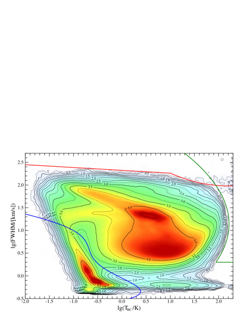
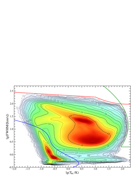
Figure 1: The distribution of the Gaussians in the $(\lg(T_{\mathrm{BC}}),\lg(\mathrm{FWHM}))$ plane. The upper panel is for the first and the lower is for the final iteration of the profile improvement. Isodensity lines are drawn in the scale of $\lg(N+1)$ with the interval of 0.25. The thick lines indicate the selection criteria used in the final iteration.

We use the results of the Gaussian decomposition to search for spurious features in the averaged profiles of the HEALPix grid. To accomplish this, we start with the frequency distributions of the obtained parameters of the positive Gaussians in $(\lg(T_{\mathrm{BC}}),\lg(\mathrm{FWHM}))$, $(V_{\mathrm{C}},\lg(\mathrm{FWHM}))$ and $(V_{\mathrm{C}},\lg(T_{\mathrm{BC}}))$ planes (Figs. 1 – 3). In the plots, we identify the regions, populated by the outliers, which in one or another way differ from the components of the main distribution and choose numerical criteria for the recognition of the corresponding Gaussians. The definition of the selection criteria is mainly based on the $(\lg(T_{\mathrm{BC}}),\lg(\mathrm{FWHM}))$ and $(V_{\mathrm{C}},\lg(\mathrm{FWHM}))$ plots, and the $(V_{\mathrm{C}},\lg(T_{\mathrm{BC}}))$ plot is used mostly for additional checking. The obtained criteria, together with those described in Sections 2.4, 2.7 and 2.8, were modified in every iteration. Figs. 1 – 3 give the frequency distributions of the Gaussian parameters in the initial (GASS II, upper panels) and final (GASS III, lower panels) versions of the data together with the final selection criteria (thick lines). We can see which kinds of Gaussians are considered spurious. As illustrated by the lower panels of these figures, in the final data the number of these Gaussians is reduced.

We used the parameters of the selected suspicious Gaussians to define a profile badness with the aim of minimizing this parameter. The badness is defined as a sum of the areas under these Gaussians. If a given Gaussian is selected by more than one criterion, its area is considered only once. The areas of the Gaussians are calculated for the velocities covered by the observed profile. Of course, these criteria are rather subjective, but they are used only for identifying the problematic profiles and for the general assessment of the degree of contamination of the averaged profiles with the spurious features. The modification of the database is done on the basis of the study of the actual profiles, as described in Sect. 3.2. The results from the Gaussian decomposition are used as guides, pointing to the areas to study. Therefore, the precise values of the criteria only influence the type and number of the problems found, but do not directly influence the corrections made in the database.

For the badness estimates of the profiles, we use six types of criteria:

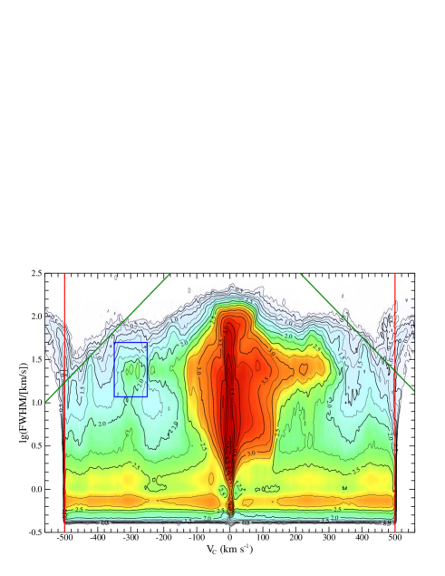
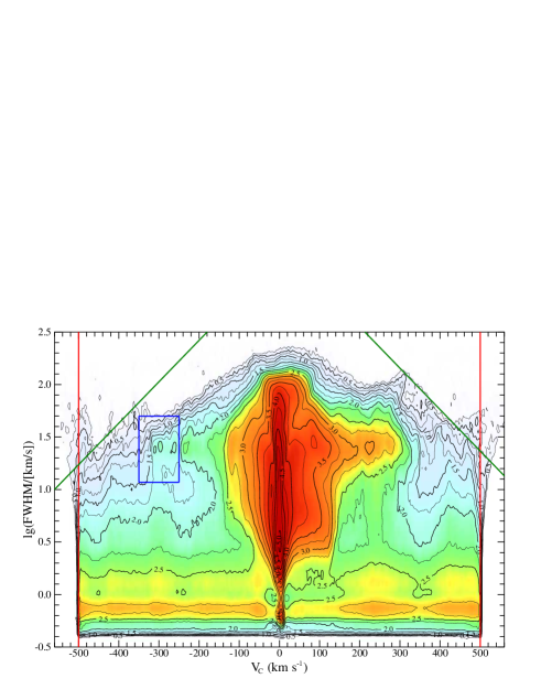
Figure 2: As Fig. 1, with the exception of the distribution of the Gaussians in the $(V_{\mathrm{C}},\lg(\mathrm{FWHM}))$ plane.

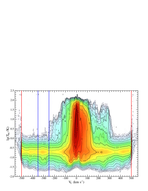
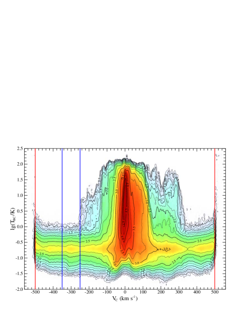
Figure 3: As Fig. 1, with the exception of the distribution of the Gaussians in the $(V_{\mathrm{C}},\lg(T_{\mathrm{BC}}))$ plane.

1. This criterion is based on the negative Gaussians in the decomposition of the H i profiles. It detects deviations of the profiles below the $T_{\mathrm{B}}=0\leavevmode\nobreak\ \mathrm{K}$ line. Often these deviations are caused by an incorrect baseline. To protect real self-absorption features in the profiles near the Galactic center against rejection, we consider only the negative Gaussians with central velocities $|V_{\mathrm{C}}|>5\leavevmode\nobreak\ \mathrm{km\,s}^{-1}$. However, sometimes other absorption features can be found. Most of the Gaussians, describing this absorption have $-70<V_{\mathrm{C}}<40\leavevmode\nobreak\ \mathrm{km\,s}^{-1}$, $T_{\mathrm{BC}}<-1\leavevmode\nobreak\ \mathrm{K}$ and $\mathrm{FWHM}<12\leavevmode\nobreak\ \mathrm{km\,s}^{-1}$. We do not consider these components as spurious either. The areas under all other negative Gaussians are added to the badness of the corresponding profiles.

2. The Gaussians, whose centers lie outside the velocity range covered by GASS, or whose centers are inside this range, but at the edge of the profile the Gaussian still has $T_{\mathrm{B}}>0.5\leavevmode\nobreak\ \mathrm{K}$. These Gaussians are mostly caused by a bad baseline near the bandpass edges. The in-band frequency switching technique, which causes significant uncertainties at high velocities, is responsible. The selection criterion is indicated in Figs. 2 and 3 with the thick red vertical lines at $|V|=500\leavevmode\nobreak\ \mathrm{km\,s}^{-1}$.

3. The Gaussians above the slanted green lines in Fig. 2. Broad high-velocity profiles are not likely to be genuine since we know from HIPASS observations that this population of high-velocity clouds does not exist (Putman et al. 2002). Inspection of the profiles with such components has demonstrated that these Gaussians are frequently caused by baseline uncertainties near the profile edges and therefore this criterion somewhat extends, but partly duplicates our second criterion.

4. The Gaussians above the red line in Fig. 1 are mostly caused by two kinds of baseline problems. Some of them fit very wide but weak wings of the main emission peaks in the profiles, which may be caused by the incorrectly determined baseline near $V_{\mathrm{C}}=0\leavevmode\nobreak\ \mathrm{km\,s}^{-1}$. This interpretation is supported by the fact that these wings are considerably reduced in the final data set. The Gaussians in the rightmost part of the figure once again represent the relatively poorly determined components, mostly behind the edges of the observed profiles and therefore this criterion partly duplicates the second and the third criterion.

5. The Gaussians that are located to the right of the green line in Fig. 1. The measured values of the brightness temperatures in the GASS are all less than $160\leavevmode\nobreak\ \mathrm{K}$, but some Gaussians are considerably higher than that and must therefore correspond to some specific features in the profiles. High components, which also have relatively large widths can only have their centers outside the velocity range covered by GASS, and therefore this criterion duplicates the second and third criterion, and also sometimes the fourth. As a rule, very narrow, but high Gaussians have their centers between the velocities, corresponding to the receiver channels. These components usually represent the very steep edges of the absorption features in the profiles and therefore cannot be considered as completely spurious.

6. The Gaussians located on the left-hand side of the blue curve in Fig. 1. These are narrow and weak components with small areas under them. Most of these Gaussians are caused by the fact that during the decomposition we prefer to decompose the strongest random noise peaks into Gaussians rather than losing a part of the signal. On average, this choice generates less than one small Gaussian per decomposed profile. However, occasionally some profiles contain tens of weak and narrow components. In most cases, this happens when the character of the residuals of the decomposition is considerable different in the baseline and signal regions of the profile. Two main causes of these differences are the presence of moderate RFI at brightness temperatures $T_{\mathrm{B}}>0.5\leavevmode\nobreak\ \mathrm{K}$ and the correlator failures. Actually, the first signs of the presence of the latter problem were discovered just through the application of this selection criterion. As these are very small Gaussians, and, in general, the number of such Gaussians per profile is more important than the area under them, for this criterion, the badness is calculated by adding their total number per profile to the usual sum of the areas under selected Gaussians.

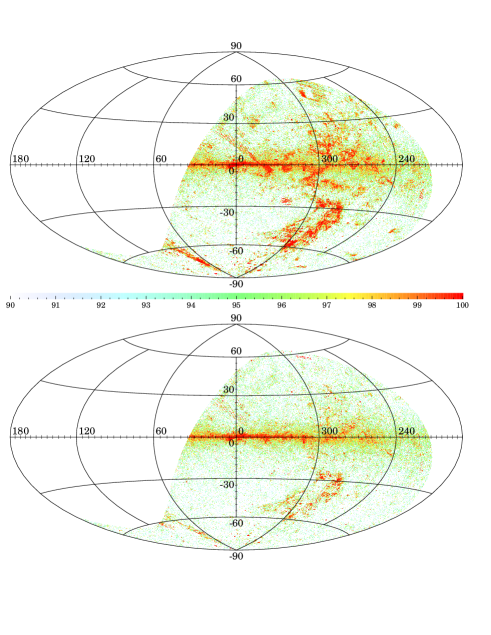
Figure 4: The sky distribution of the most problematic profiles in the initial (upper panel) and final (lower panel) database. The color scale corresponds to the rank of the badness in the initial data, with 100% corresponding to the most and 0% to the least problematic profile. In the lower panel, each profile is plotted with the color that corresponded, in the upper panel, to the value of the badness of this profile in the final database.

After using the six criteria described above, and correcting the data on account of the problems detected by these criteria, we created a short movie by computing the sky distribution of the brightness temperatures at running velocities from our latest Gaussian decomposition of the HEALPix profiles. In this movie, the observational noise is greatly suppressed and even weak features, approximated by Gaussians, become clearly visible. In general, the movie appeared as expected, but in the velocity range of $-350<V<-250\leavevmode\nobreak\ \mathrm{km\,s}^{-1}$ we found a number of fields with rather fuzzy borders, which contained brightness enhancements of the order of $T_{\mathrm{B}}=0.075\leavevmode\nobreak\ \mathrm{K}$.

We decided to study these “stains” on our movie in greater detail, but the separation of the Gaussians, responsible for the enhancements, was not easy. First, we determined that the typical central velocities and widths of corresponding Gaussians fall into the blue rectangle in Fig. 2 ($-350<V_{\mathrm{C}}<-250\leavevmode\nobreak\ \mathrm{km\,s}^{-1}$ and $11.7<\mathrm{FWHM}<50\leavevmode\nobreak\ \mathrm{km\,s}^{-1}$), but similar components may also represent high-velocity clouds (HVCs; the horizontal band of enhanced frequency of the Gaussians at about $\lg(\mathrm{FWHM})=1.4$) and there is also an enhancement of narrower components at the same velocities down to the very narrow Gaussians, mostly representing the higher peaks of the random noise (orange bands at about $\lg(\mathrm{FWHM})=-0.15$ and $0.1$).

To exclude the noise from the following discussion, we use the cluster analysis, as described in Sec. 2 of Haud (2010), and consider in the following only the clusters of at least three Gaussians in which the average velocities and $\mathrm{FWHM}$ fall inside the limits, indicated in Figs. 2 and 3 by blue lines. In doing so, we assume it to be rather improbable that three neighboring profiles have similar random noise peaks. We also reject all small clusters at great distances from the large clusters at the centers of the stains. To exclude the HVCs, we use the fact that at considered velocities the HVCs are mostly located in the longitude range $5\degr<l<130\degr$ and the stains were outside this region. However, to be on the safe side, we also do not search for stains at up to $15\degr$ around the South Galactic pole, $20\degr$ around the Galactic center, and $3\degr$ around the Galactic plane.

As a result, we obtained a list of 1172 clusters, containing 24867 Gaussians, which we could use for the search of problematic data dumps. It turned out that observations between January and June 2005 are affected by low-level RFI. This period is part of the first coverage with declination scans. The corresponding data from the second coverage, scanning in RA, were found to be unaffected by this kind of RFI. We flagged all channels for dumps from the first coverage, which contributed to positions in the list of problematic Gaussians. The RFI usually affects most of the multibeam systems at the same time; for this reason the flagging was applied simultaneously to all receivers whenever valid data from the second coverage were available. We corrected 201929 individual dumps by flagging 14720316 affected channels in total.

As the cluster analysis is a rather labor consuming endeavor, it was applied only to the version of the data obtained after using the first six criteria. For the calculations of the badness used in Figs. 4 – 6, the selections of velocities, line widths, and sky coordinates for the stains, are applied to individual Gaussians in the decompositions of the initial and final data sets. This adds some contamination by random noise to these figures. Nevertheless, examples of the described stains are well visible in the upper panel of Fig. 4 around $(l,\leavevmode\nobreak\ b)=(291\degr,\leavevmode\nobreak\ 51\degr)$, $(229\degr,\leavevmode\nobreak\ 24\degr)$, $(263\degr,\leavevmode\nobreak\ 4\degr)$, $(207\degr,\leavevmode\nobreak\ -40\degr)$ and $(198\degr,\leavevmode\nobreak\ -57\degr)$. In the upper panel of Fig. 2 the vertical enhancement in the distribution of Gaussians, similar to that discussed above, is visible also around $V_{\mathrm{C}}=234\leavevmode\nobreak\ \mathrm{km\,s}^{-1}$. The weaker enhancements exist near $V_{\mathrm{C}}=-420$, $423$, $-476$, and $470\leavevmode\nobreak\ \mathrm{km\,s}^{-1}$. We checked corresponding movie frames, but as no obvious stains were found, we did not attempt to flag the corresponding regions of the data dumps.

The results of the searches of the spurious features in the initial and final profiles are presented in Figs. 4 – 6. The upper panel of Fig. 4 illustrates the sky distribution of the 10% of the profiles with the highest badness values in the initial database. Here the colors of the points represent the ranks of the corresponding badness values. The lower panel is for the final data and the final badness of each profile is given with the same color as was used for the corresponding value in the upper panel. Therefore, if the color of some profile in the lower panel is blue shifted with respect to the color of the same profile in the upper panel, according to our criteria this profile in the final data is improved in comparison with its initial version. Shifts toward red indicate that the corresponding profiles have become even more problematic. Figures 4 and 5 show that the profiles in the Galactic plane have the lowest quality (highest badness). There are two reasons for this: the system noise is highest in this region, and the baseline is most uncertain because the fit there has to span the largest velocity intervals. To ensure constant quality at all latitudes, it would have been necessary to increase the integration time at low latitudes during observations.

The badness values for the most problematic profiles are given in Fig. 6. We can see that about 5 000 profiles were considerably improved (according to our criteria) and smaller improvements were obtained in many more cases. The bumps in the red curve for the initial badness distribution can be identified with residual instrumental problems in GASS II. The improved baseline algorithm and the rejection of the dumps with the worst correlator failures has led to a general decrease in the badness. For GASS III, the slope of the green log-log relation in Fig. 6 is approximately constant. Since significant wiggles in the green line are missing, we may conclude that the most severe problems have probably been removed.

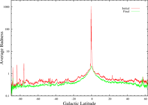
Figure 5: The average badness of the profiles at different Galactic latitudes in the initial and final data.

Figure 6: The comparison of the badness of the most problematic profiles in the initial and final database. The rank of the profile badness in the corresponding database is used as an abscissa. On this axis, the value of 640 126 corresponds to 90% on the color scale of Fig. 4 and 1 corresponds to 100%.

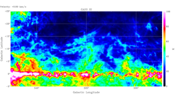
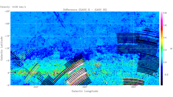
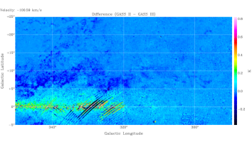
Figure 7: Top: the GASS III HI emission at ${\rm v_{\mathrm{lsr}}}=0.0$ km s^-1. For comparison, we show errors that have been removed from GASS III; in the middle at the same velocity, at the bottom for $v_{\mathrm{lsr}}=-100.6$ km s^-1. This comparison demonstrates that most of the instrumental effects are strongly frequency dependent.

3.2 Visualization

Parallel to checking the results of the Gaussian analysis, we calculated 3-D FITS cubes for visual inspection. To demonstrate the progress in cleaning the GASS database, we present a few channel maps.

Figure 7 shows a region that is typical for strong H i  emission in the Galactic plane. The GASS III image for $v_{\mathrm{lsr}}=0.0$ km s^-1  is displayed on top. Below we show changes in comparison to GASS II. Most obvious are scanning stripes in the right ascension or declination direction that originate from RFI or correlator failures. At $l\sim 315\degr,b\sim 3\degr$ a typical RFI footprint is visible, most of the other isolated spots are due to RFI. The RFI footprints tend to shift with velocity along the scanning direction while the stripes show oscillating intensities. Close to the Galactic plane we find an average positive baseline offset of $\delta T_{B}\sim+100$ mK which is surrounded by a region with an offset of $\delta T_{B}\sim-50$ mK. Offsets of this kind are slowly variable and caused by imperfect baseline fitting in GASS II as discussed in Sect. 2.4. The bottom of Fig. 7 at ${v_{\mathrm{lsr}}}=-100.0$ km s^-1shows that the striped structures are less prominent at high velocities but baseline offsets are also present there. In total, 2.2% of the dumps within this data cube have been discarded. For the whole survey about 1.5% of the dumps are affected.

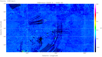
Figure 8: Instrumental errors, eliminated from GASS III, at $v_{\mathrm{lsr}}=0.0$ km s^-1, typical for high Galactic latitudes. The stripes are in scanning direction, at $l\sim 288\degr,b\sim-25\degr$ a typical RFI footprint is visible, some regions show baseline offsets.

Figure 8 displays corrected errors in a region typical for high latitudes. At $l\sim 288\degr,b\sim-25\degr$ we find an RFI footprint. Stripes at high latitudes are in general less prominent due to low H i  brightness temperatures (the correlator problems were found to scale with line intensity). The south pole is at $l\sim 303\degr$, $b\sim-27\degr$, and we demonstrate how the stripes are related to the telescope scanning in right ascension or declination.

Figure 9 demonstrates improvements in the baseline. It shows some low-intensity emission features at ${v_{\mathrm{lsr}}}=320.0$ km s^-1, belonging to the leading arm of the Magellanic system. Along these features baseline offsets around -50 mK are visible, which were caused in GASS II by inappropriate baseline estimates derived from the LAB survey (see Sect. 2.4 for details). In GASS III, baseline biases for emission features of this kind are removed. Weak sources are better isolated from the background noise, which can lead to a doubling in area covered by these weak features (Verena Lüghausen, private communication).

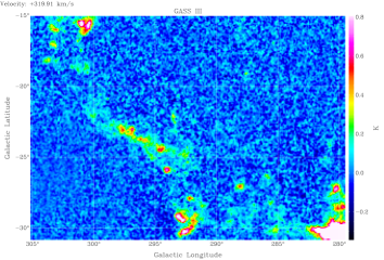
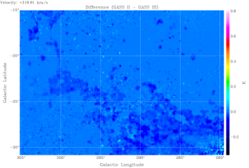
Figure 9: Top: weak emission in the leading arm region. Bottom: RFI at individual positions and extended regions with systematical baseline offsets that have been removed.

For a more extended overview about improvements that were obtained with our current analysis, we calculated FITS cubes for the brightness temperature distribution of the GASS II and III versions and subtracted our current $T_{B}$ results from the previous data release (Paper II). We generated a movie that can be downloaded: https://www.astro.uni-bonn.de/hisurvey/gass/GASS2-3.avi. To focus on low-level emission, we clipped the data for $-0.05<T_{B}<0.2$ K. The flicker visible for some of the features originates from channel-to-channel fluctuations that existed for the GASS II data release.

For a display of the remaining problems, we generated another movie with the same clip levels for the GASS III data release: https://www.astro.uni-bonn.de/hisurvey/gass/GASS3noise.avi. This version emphasizes low-level emission and noise while it saturates for strong emission features. This way it is possible to observe numerous spurious low-level features that run across the sky. These features are mostly so weak that they are hardly visible in individual channel maps. Because of systematic shifts in velocity they are easily recognizable in a movie. Pale features mimic emission while dark filaments are due to ghosts. The velocity shifts are caused by the local standard of rest correction, which does not apply for terrestrial RFI. All these features are so weak that they are not recognizable by our cleaning algorithm.

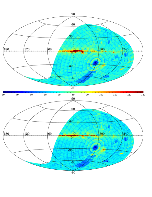
Figure 10: Mean rms noise level in mK across the sky obtained from the HEALPix database. Top: GASS II, bottom: GASS III.

Figure 10 displays the mean rms uncertainties within a single velocity channel as determined from the HEALPix database for the initial GASS II database (top) in comparison to the final result (bottom). Overall we find that the elimination of unreliable data leads to a general decrease in the average rms fluctuations by 2.7%. We only find a slight increase for very few places. To understand why the elimination of flagged data leads to a decrease in the uncertainties, we need to take into account that flagged data usually deviate significantly from a random distribution. Elimination of bad data leads to an improved error distribution, approaching the expected white noise.

Figure 10 only shows mean rms uncertainties. Depending on flagging of individual velocity channels according to Eq. 3, the noise may be different for those regions or velocities that were seriously affected by RFI or other instrumental problems. For FITS data products, the noise depends on the map parameters (see Paper II, Sect. 6), and for this reason the noise level of Fig. 9 in Paper II differs from that of Fig. 10.

4 Calibration issues

4.1 Comparison between GASS and LAB

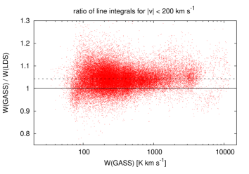
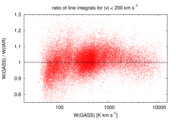
Figure 11: Comparison of line integrals $W_{\mathrm{GASSIII}}/W_{\mathrm{LAB}}$ derived for $|v_{\mathrm{lsr}}|<200.0$ km s^-1from the LAB survey and from GASS III. We distinguish between data observed with the 25-m Dingeloo telescope (LDS, top) and with the 30-m IAR telescope at Villa Elisa (IAR, bottom). The dashed lines are for $W_{\mathrm{GASSIII}}/W_{\mathrm{LDS}}=1.0426$ (top) and $W_{\mathrm{GASSIII}}/W_{\mathrm{IAR}}=1.0096$ (bottom).

To compare the complete GASS III with other surveys for quality control, there is essentially only the LAB survey available. We therefore generated for both surveys a database of average profiles on a HEALPix grid with $N_{\mathrm{side}}=128$. These profiles were then integrated for $|v|<200$ km s^-1for comparison.

The calibration of the GASS was independent from the LAB (see Sect. 4 of Paper II), however, baselines of GASS II were derived by bootstrapping from the LAB survey, resulting in possible biases. The GASS III has improved baselines that were derived iteratively without using LAB data. Therefore LAB and GASS III are independent from each other.

The LAB survey was observed with two different telescopes, and accordingly, we compare both data sets separately. Declinations $\delta>-27\hbox{$.\!\!^{\circ}$}5$ were observed with the 25-m Dingeloo radio telescope (Leiden-Dwingeloo-Survey, LDS, Hartmann & Burton 1997), while declinations $\delta\leq-27\hbox{$.\!\!^{\circ}$}5$ were observed with the 30-m telescope of the Instituto Argentino de Radioastronomía (IAR) by Bajaja et al. (2005).

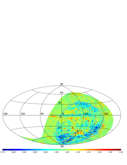
Figure 12: Spatial distribution of $W_{\mathrm{GASSIII}}/W_{\mathrm{LAB}}$. Declinations $\delta\geq-27\hbox{$.\!\!^{\circ}$}5$ (indicated by the dashed line) were observed with the Dwingeloo telescope and have systematically high $W_{\mathrm{GASSIII}}/W_{\mathrm{LAB}}$ values.

Figure 11 displays the ratios of the line integrals $W_{\mathrm{GASSIII}}/W_{\mathrm{LDS}}$ (top) and $W_{\mathrm{GASSIII}}/W_{\mathrm{IAR}}$ (bottom) as a function of the line integrals $W_{\mathrm{GASSIII}}$. Fitting average quotients, we obtain $W_{\mathrm{GASSIII}}/W_{\mathrm{LDS}}=1.0426(\pm 0.0002)$ and $W_{\mathrm{GASSIII}}/W_{\mathrm{IAR}}=1.0096(\pm 0.0004)$. For the whole LAB survey, we obtain $W_{\mathrm{GASSIII}}/W_{\mathrm{LAB}}=1.0254(\pm 0.0002)$. The scatter visible in Fig. 11 is considerable, but because of the large number of data points ($n=48824$ and $n=52912$ for LDS and IAR, respectively) the appearance is somewhat biased by outliers. The quotients are well defined and show systematic differences between LDS and IAR.

To disclose whether there might be a systematic trend in the spatial distribution of these inconsistencies we plot in Fig. 12 $W_{\mathrm{GASSIII}}/W_{\mathrm{LAB}}$ in Galactic coordinates. Different systematic effects for the ratios $W_{\mathrm{GASSIII}}/W_{\mathrm{LAB}}$ for the LDS and IAR survey are obvious.

For declinations $\delta>-27\hbox{$.\!\!^{\circ}$}5$, the region covered by the LDS survey, there appear to be fluctuations without a clear trend. For lower declinations, covered by the IAR, there is a range with systematically low values of $W_{\mathrm{GASSIII}}/W_{\mathrm{IAR}}$ but there are also apparently no systematic trends. Fluctuations for declinations $\delta\leq-27\hbox{$.\!\!^{\circ}$}5$ are significantly larger than for declinations above this limit. We find blocky structures in Fig. 12, and in Fig. 8 at the bottom of Paper II, indicating that the errors are correlated with the observing strategy. For the IAR, a grid of 5 by 5 positions was observed. The blocky structure is found to be frequency dependent, the IAR data may therefore contain some residual stray radiation or baseline problems.

4.2 Comparison with other telescopes

The GASS brightness temperature scale may also be compared with calibrations at IAU standard position S8 (Williams 1973) as determined by Kalberla et al. (1982) for the Effelsberg telescope. For the S8 line integral within the velocity range $-5.1<v_{\mathrm{lsr}}<22.3$ km s^-1  , we obtain $W_{\mathrm{GASSIII}}/W_{\mathrm{Eff}}=1.033\pm 0.005$. Comparing the peak temperatures, we get $T_{\mathrm{GASSIII}}/T_{\mathrm{Eff}}=1.041\pm 0.01$. We conclude that the GASS III brightness temperature scale is about 4% higher in comparison to the scale determined by the Dwingeloo and Effelsberg telescopes in the northern hemisphere.

The Dwingeloo brightness temperature scale dates back to the calibration by Baars et al. (1977) against Tau A and is within uncertainties of $<1\%$ consistent with the LDS scale (Kalberla & Haud 2006). A similarly good agreement was found with the independently determined Effelsberg scale (Kalberla et al. 1982).

Apparently, there is a systematic mismatch between the calibrations in the northern and southern hemispheres. We use results from an independent absolute calibration obtained with the Green Bank Telescope (GBT) with the hopes of shedding light on the origin of this discrepancy. Boothroyd et al. (2011, Sects. 5.2, 7.4, 8.1, and 8.2) compare their calibration with Effelsberg and LAB data. They find for S8 $W_{\mathrm{Eff}}/W_{\mathrm{GBT}}=1.018\pm 0.018$, $W_{\mathrm{LAB}}/W_{\mathrm{GBT}}=1.019\pm 0.007$, and for S6 $W_{\mathrm{LAB}}/W_{\mathrm{GBT}}=1.015\pm 0.010$. In addition, a number of pointed observations yield $W_{\mathrm{LAB}}/W_{\mathrm{GBT}}=1.0288\pm 0.0012$. Thus the LAB and Effelsberg brightness temperature scales are consistently $2-3$% higher in comparison with the GBT. This implies, however, that the GASS brightness temperature scale exceeds the GBT scale by 6-7%.

After this more extended comparison of differences in the calibration between several telescopes, we arrive at the conclusion that there must be a systematic bias in calibration between the northern and southern hemisphere. The discrepancy most probably reflects calibration uncertainties that remained undetected previously since observers in both hemispheres tend to use different standard positions for their internal calibration: S7 in the north and S9 in the south. Systematic calibration errors are, in any case, hard to estimate. We need to accept uncertainties of 1 – 3%.

On one hand, we have in the north the Dwingeloo, Effelsberg, and GBT telescopes, which have within one or two percent a common consistent brightness temperature scale. In the south, the calibration between the IAR and the Parkes telescopes is also very consistent within one percent. The problem is that both scales differ systematically by 3 – 4%. This discrepancy exceeds the expected uncertainties. To obtain a consistent temperature scale, we propose to match the GASS brightness temperatures to the LAB survey by scaling down the GASS brightness temperatures by a factor of 0.96. This scale would also be consistent with the Effelsberg calibration (Kalberla et al. 1982) and the remaining deviations from the GBT scale would be limited to $\sim 2$%.

5 Summary

The second edition of the GASS has been in use since 2010 and it has become evident that some instrumental problems remained to be solved. We developed an iterative procedure to remove these problems as far as possible.

In the first instance, we generate a database of profiles averaged on a HEALPix grid with $N_{\mathrm{side}}=1024$. For quality control these profiles are decomposed into Gaussian components. When fitting instrumental baselines of individual telescope dumps we use priors from the HEALPix database. Next we calculate whether the rms deviations from the nearest average HEALPix profile are acceptable for each dump. We search the dumps for oscillations caused by correlator failures or RFI. Bad dumps are marked and excluded from calculating averages in the further iterations. Eventually, we generate 3-D FITS cubes for visual inspection and proceed to calculate a new version of improved averages for the next iteration. In total, we need to exclude about 1.5% of the telescope dumps for an improved version of the GASS. Examples for the improvements are given in Figs. 7 to 9. Essential for this progress was the combined analysis of Gaussian components and the visual inspection of 3-D FITS data cubes for the complete survey.

We compare GASS III with the LAB survey and find differences that most probably indicate systematical deviations in calibration. For declinations $\delta>-27\hbox{$.\!\!^{\circ}$}5$, the GASS III brightness temperature is 4% too high in comparison with the Dwingeloo and Effelsberg scales, south of this region the GASS III scale is 1% too high in comparison with the IAR survey. In comparison to the GBT calibration we even find a discrepancy of 6-7%.

Data products from GASS III, compatible with the GASS II web-interface, are available at http://www.astro.uni-bonn.de/hisurvey/.