Phenomenological implications of a minimal F-theory GUT with discrete symmetry

Athanasios Karozas^† , Stephen F. King^⋆ , George K. Leontaris^† , Andrew K. Meadowcroft^⋆

^⋆ School of Physics and Astronomy, University of Southampton,

SO17 1BJ Southampton, United Kingdom

^† Physics Department, Theory Division, Ioannina University,

GR-45110 Ioannina, Greece

We discuss the origin of both non-Abelian discrete family symmetry and Abelian continuous family symmetry, as well as matter parity, from F-theory SUSY GUTs. We propose a minimal model based on the smallest GUT group $SU(5)$, together with the non-Abelian family symmetry $D_{4}$ plus an Abelian family symmetry, where fluxes are responsible for doublet-triplet splitting, leading to a realistic low energy spectrum with phenomenologically acceptable quark and lepton masses and mixing. We show how a $Z_{2}$ matter parity emerging from F-theory can suppress proton decay while allowing neutron-antineutron oscillations, providing a distinctive signature of the set-up.

1 Introduction

F-theory [1] models have attracted considerable interest over the recent years [2]-[9]. For example, Supersymmetric (SUSY) Grand Unified Theories (GUTs) based on $SU(5)$ has been shown to emerge naturally from F-theory [10]-[25]. However, in the F-theory context, the $SU(5)$ GUT group is only one part of a larger symmetry. The other parts manifest themselves at low energies as Abelian and/or non-Abelian discrete symmetries, which can be identified as family symmetries, leading to significant constraints in the effective superpotential.

In this paper we review the basic mechanisms responsible for the origin of both non-Abelian discrete family symmetry and Abelian continuous family symmetry, as well as matter parity, from F-theory SUSY GUTs, before piecing together the first realistic example model of its kind which includes all three types of symmetries. In order to make this paper self-contained, and hopefully useful to model builders not familiar with F-theory, we shall include necessary introductory material, as well as a discussion of basic features which will be obvious to F-theory experts, but may be new to the expected readership of this paper. Thus we begin with a fairly general introduction (or a reminder for the experts) on how symmetries of any kind can emerge from F-theory (for more details see reviews [26]-[30]).

As a basic starting point, it is worth remarking that F-theory is a non-perturbative formulation of type IIB string theory invariant under a $SL(2,Z)$ symmetry (the $S$-duality) which attains a geometric realisation. Current F-theory constructions are based on an elliptically fibred internal space where the complex modulus of the elliptic fiber is a combination of the axion and dilaton fields $\tau=C_{0}+ie^{-\phi}$, i.e., the two scalars of the type IIB bosonic spectrum (see Figure 1). This way, F-theory can be considered as a 12-dimensional string theory compactified on a torus characterised by the above modulus $\tau$. Algebraically, the fibration is described by a birationally equivalent complex cubic equation, the so called Weierstraß  model [2, 3, 4]. Depending on the specific structure of its coefficients, at certain points of the fibration the torus degenerates and the fibration becomes singular. All possible singularities have been classified with respect to the vanishing order of the coefficients (polynomials) and the discriminant of the Weierstraß  equation. It was shown long time ago [31] (see also recent works [32, 33]) that these singularities are of ADE type (in the Cartan classification of non-Abelian groups), the highest being the ${E}_{8}$ exceptional group.

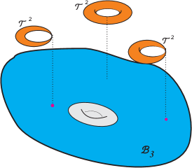
Figure 1: A pictorial representation of a Calabi fourfold, which exhibits elliptic fibration over a threefold base, $B_{3}$. The fibration is manifest as a 2-Torus at every point in the base, as shown. The modulus of the torus at each point is related to the axio-dilaton profile, $\tau=C_{0}+i/g_{s}$. Where the fibre degenerates, the presence of a D7-brane orthogonal to the base is indicated.

In F-theory non-Abelian gauge symmetries are linked to the singularities of the elliptic fibre. Hence, old successful GUTs based on the exceptional groups ${E}_{6,7,8}$, as well as the lower rank $SO(10)$ and $SU(5)$ ones, can be naturally realised as effective F-theory models. As such, they constitute a particularly promising component of the vast string landscape, since many parameters of the effective low energy models are determined from a few basic topological properties of the compact space associated to the geometric nature of the singularities.

However, one might object that building a model from F-theory one has to deal with complications due to the as yet unknown global geometrical structure of the internal space. Moreover, various mathematical issues of the elliptic fibrations, whose role in model building is not well understood, would further obscure physics. Despite the complicated structure of the global geometry, it is often adequate to focus on a local F-theory description where computations are simpler leading to reliable predictions of the effective model’s parameter space.

In the local approach, one may associate the GUT symmetry to a particular divisor of the elliptically fibred manifold and use techniques such as the spectral cover [3] to deal with the implications of the remaining symmetry and the topological properties of the compact space. In this context, one may determine the massless spectrum of the effective theory and all its properties under the GUT group and its quantum numbers with respect to the symmetries of the spectral cover. Furthermore from general characteristics of the compact manifold and G-fluxes [3] we can determine the chiralities of the massless spectrum.

Within the local approach, we can focus on a small patch and compute several important quantities such as the Yukawa couplings [34]-[43]. Indeed, in F-theory massless fields reside on the intersections of various D7-branes, usually called matter curves. In this picture, a massless state is described by a wavefunction which exhibits a Gaussian profile picked on the corresponding matter curve and can be determined by solving the appropriate equations of motion. The Yukawa couplings occur at triple intersections of three matter curves. Studying locally the wavefunctions’ profiles of the relevant states one is able to compute the strength of these couplings and predict the mass spectrum and (in principle) all possible interactions allowed within a specific model.

In addition to the non-Abelian sector, in F-theory effective models are endowed with Abelian and discrete symmetries which may arise either as a subgroup of the non-Abelian symmetry or from a non-trivial Mordell-Weil group associated to rational sections of the elliptic fibration. It is well known that the discrete symmetries in particular are extremely important in suppressing undesired proton decay operators and generate a hierarchical fermion mass spectrum . Furthermore, non-Abelian discrete groups were introduced to interpret the mixing properties of the neutrino sector [57, 58, 59, 60].

In the present work, then, we will focus on non-Abelian discrete symmetries emerging in the context of the spectral cover, accompanied by continuous Abelian symmetry. We continue to investigate the grid of discrete symmetries emerging as subgroups of the $SU(5)_{\perp}$ spectral cover symmetry. Motivated by the successful implementation of a class of such symmetries to the neutrino sector, we focus on the subgroups of $S_{4}$. We also show how a geometric discrete $Z_{2}$ symmetry can additionally emerge, leading to matter parity which can control proton decay operators. However, due to the basic feature of F-theory constructions with flux breaking of the GUT group yielding doublet-triplet splitting and incomplete GUT representations, the matter parity is necessarily of a new kind. In the particular example we develop, based on $D_{4}\times U(1)$ family symmetry, with an $SU(5)$ GUT group, broken by fluxes, the geometric $Z_{2}$ matter parity, while suppressing proton decay, allows neutron-antineutron oscillations, providing a distinctive signature of the set-up. To be precise, while $QLd^{c}$ is forbidden, the operator $u^{c}d^{c}d^{c}$ is present leading to $n\bar{n}$ oscillations at a calculable rate.

The layout of the remainder of the paper is as follows. In Section 2, we review the basics of F-theory GUTs based on $SU(5)$ together with additonal $U(1)^{4}$ groups, or subgroups thereof. In Section 3 we describe the Spectral Cover approach and show how a $S_{4}\times U(1)$ group can emerge from this formalism; we also discuss the origin of an additional $Z_{2}$ geometric symmetry which can play the role of matter parity. In Section 4 we clarify in some detail the action of the possible monodromy group on the matter representations, distinguishing abelian and non-abelian discrete cases. In Section 5 we show how a $D_{4}$ discrete symmetry subgroup of the $S_{4}$ can emerge. The structure of this non-Abelian discrete symmetry seems promising, so can be used to illustrate in the simplest setting many of the features of interest, and can be used as the basis for constructing a realistic model which we do in Section 6. In Section 7 we investigate the physics of baryon number violation in this model, showing how the combination of symmetries can suppress proton decay, but allows baryon number violating operators which can yield neutron-antineutron oscillations, providing a distinctive signature of our scheme. Section 8 concludes the paper.

2 F-$SU(5)$ basics with $U(1)^{4}$

In this work we are interested in $SU(5)_{GUT}$ which is the minimum GUT group accommodating the Standard Model symmetry. This is embedded in a local $E_{8}$ singularity according to, such that the massless spectrum is found in adjoint of $E_{8}$, which under the maximal decomposition of the $E_{8}\to SU(5)_{GUT}\times SU(5)_{\perp}$ decomposes as follows

$$248 \rightarrow (24,1)+(1,24)+(10,5)+(\overline{5},10)+(\overline{10},\overline{5})+(5,\overline{10}).$$ (2.1)

As expected, the $SU(5)_{GUT}$ multiplets have transformation properties under the second $SU(5)_{\perp}$. The $10$ multiplets in particular are in the fundamental of $SU(5)_{\perp}$, while the $5$-plets are in the antisymmetric of $SU(5)_{\perp}$. Depending on the geometry of the internal manifold and the fluxes, $SU(5)_{\perp}$ can be broken to an appropriate subgroup. This way, matter curves and hence, the $SU(5)_{GUT}$ representations acquire specific topological and symmetry properties inherited to the fermion families and Higgs fields.

There are a variety of symmetry options embedded in $SU(5)_{\perp}$ and our choice in this work will be dictated by observational facts. As already discussed, we will focus on non-Abelian discrete symmetries accompanying $SU(5)_{GUT}$. Nevertheless, to set the stage, it is convenient first to start with the Abelian symmetries. In this case we have the following breaking pattern

$$E_{8}\supset SU(5)\times SU(5)_{\perp}\rightarrow SU(5)\times U(1)_{\perp}^{4}.$$ (2.2)

Thus, the $SU(5)_{GUT}$ matter content transforms non-trivially under the Cartan subalgebra of $SU(5)_{\perp}$ with weight vectors $t_{1,...,5}$ satisfying

$$\sum_{i}t_{i}=0.$$ (2.3)

Under the above notation the matter curves accommodating the $SU(5)$ representations are labelled as follows

$$10_{t_{i}},\;\overline{10}_{-t_{i}},\;\bar{5}_{t_{i}+t_{j}},\;5_{-t_{i}-t_{j}},\;1_{t_{i}-t_{j}}$$ (2.4)

where, due to antisymmetry, the indices of the fiveplets must differ $i\neq j$. As a result, the ‘charges’ $t_{i}$ distinguish the various matter curves and eventually the fermion generations associated to some of them.

In principle the superpotential can be constrained by all these four $U(1)$’s, however monodromy actions reduce their number while the constraints are adjusted accordingly. In general, monodromies are necessary in order to allow a diagonal tree-level coupling for the top-quark. Indeed, any $SU(5)_{GUT}$ invariant trilinear coupling should respect the $U(1)$ symmetries. In this case, the following tree-level couplings can be realised

$$10_{t_{i}}10_{t_{j}}5_{-t_{i}-t_{j}},\;10_{t_{i}}\bar{5}_{t_{j}+t_{k}}\bar{5}_{t_{l}+t_{m}},\;10_{t_{i}}\overline{10}_{-t_{j}}1_{t_{j}-t_{i}}.$$ (2.5)

The first term contributes to the up-quark sector, while the $U(1)$ invariance is guaranteed by the fact that the ‘charges’ sum up to zero: $\{t_{i}\}+\{t_{j}\}+\{-t_{i}-t_{j}\}=0$. The second term is $U(1)$ invariant due to (2.3) provided all indices $i,j,k,l,m$ are different. The third term might prove useful to provide heavy masses to extra tenplet pairs.

A few remarks are in order. Firstly, if all $U(1)$ symmetries are unbroken, the coupling $10_{t_{i}}10_{t_{j}}5_{-t_{i}-t_{j}}$ contributes only to non-diagonal mass terms, thus there is no diagonal top-quark coupling as required. The reason is that due to antisymmetry we must have $i\neq j$. Secondly, it is not possible to generate a term coupling additional fiveplet-antifiveplet pairs, since this would require singlets with charges ${t_{k}+t_{l}-t_{i}-t_{j}}$.

$$\bar{5}_{t_{i}+t_{j}}5_{-t_{k}-t_{l}}1_{t_{k}+t_{l}-t_{i}-t_{j}}$$ (2.6)

Such singlets might exist only outside the $E_{8}$ whose heterotic duals might be associated with non perturbative states [61].

However, as already mentioned, there is an action on $t_{i}$’s of a non-trivial monodromy group. The minimal possibility is a ${Z}_{2}$ monodromy, $t_{1}\leftrightarrow t_{2}$, i.e, the one which identifies two $U(1)$ charges. This leads to an identification of the corresponding matter curves, where the tenplets reside. As a result, the coupling

$$10_{t_{1}}10_{t_{2}}5_{-t_{1}-t_{2}}\to 10_{t_{1}}10_{t_{1}}5_{-2t_{1}}$$

becomes diagonal and a top-quark mass is obtained from a tree-level coupling.

Moreover, certain couplings of the type $5\cdot\bar{5}\cdot 1$ which within the original symmetry structure would require a singlet of the type given in (2.6), after the monodromy action are in principle allowed with singlets within $E_{8}$ matter. Indeed, for a $Z_{2}$ monodromy such that $t_{j}=t_{k}$ for example, (2.6) becomes

$$\bar{5}_{t_{i}+t_{j}}5_{-t_{j}-t_{l}}1_{t_{l}-t_{i}}$$

Therefore, in contrast to the singlet field of the term (2.6), here the same fiveplet pair receives a mass with a singlet vev $1_{t_{l}-t_{i}}$ which is embedded in $E_{8}$. We observe that, monodromies are capable of generating important Yukawa terms (like $\mu$-term), making -at least in some cases- the additional singlets redundant.

As already noted, the reduction of the accompanying symmetry to the maximum number of abelian factors $SU(5)_{\perp}\to U(1)^{4}$ discussed above is just one of a plethora of possibilities. There exists a variety of groups embedded in $SU(5)_{\perp}$ which can in principle appear in the effective theory. These include non-Abelian groups $SU(n)$ with $n<5$, or discrete ones, as well as combinations of both of them.

As for the corresponding geometrical picture, in the spectral cover approach, the Higgs bundle over the GUT divisor is described by a five degree polynomial, $\sum_{k}b_{k}s^{5-k}=0$, whose roots are associated to the $t_{i}$ charges and its coefficients carry the information from the background geometry. These roots may fall into a variety of monodromy groups and as long as the discrete options are concerned, this can be a Galois subgroup of the Weyl group $W(SU(5)_{\perp})=S_{5}$. This includes the alternating groups ${A}_{n}$, the dihedral groups ${D}_{n}$ and cyclic groups ${Z}_{n}$, $n\leq 5$ and the Klein four-group ${Z}_{2}\times{Z}_{2}$. We will discuss these options in the next sections.

3 The Spectral Cover approach

Before going into our phenomenological investigation of the available list of discrete symmetries accompanying the $SU(5)$ GUT, in this section we recapitulate a few general aspects of the spectral cover approach.

F-theory is characterised as a Calabi-Yau complex fourfold, elliptically fibred over a three complex dimensional space, $B_{3}$ with three complex coordinates $x,y,z$, corresponding to the six compact spatial dimensions. The GUT gauge group lives on the del Pezzo surface with coordinates $x,y$. The elliptic fibration is described mathematically by the Weierstraß  equation,

$$y^{2}=x^{3}+f(z)x+g(z)\,,$$ (3.1)

where $f(z)$ and $g(z)$ are eighth and twelfth degree polynomials in $z$, the coordinate normal to the GUT surface. The fibre of this space has singularities that can be classified by examining the zeroes of the discriminant and the vanishing order of the functions $f(z),g(z)$ of equation (3.1). These singularities have been classified by Kodaira [31] (see also  [32, 33]), and are in general associated with non-Abelian gauge groups, with the largest allowed symmetry group being the exceptional group $E_{8}$. In the current work we will be assuming an $SU(5)_{GUT}$, which has a corresponding commutant with the $E_{8}$ of $SU(5)_{\perp}$, called the perpendicular group. It is within this perpendicular $SU(5)_{\perp}$ group that the extra symmetries, commuting with the $SU(5)_{GUT}$, reside.

3.1 Spectral Cover of the 10s

The spectral cover equation for the $10$s of the $SU(5)$ GUT group are defined by a fifth order polynomial. In this scenario, the Weierstraß  equation can be recast into the so-called Spectral Cover equation [6]:

$$C_{5}:\,\sum_{k}^{5}b_{k}s^{5-k}=0\,,$$ (3.2)

where $b_{k}$ are holomorphic sections and $s$ is an affine parameter derived from the coordinates on the underlying manifold. From Group theory we know that $SU(5)_{\perp}$ can be decomposed into four $U(1)$ factors. As such we can suppose that the spectral cover be allowed to factorise into a product of irreducible parts. For example, we will take an interest in the case where one of the roots factorises out to a linear part:

$$C_{5}\rightarrow C_{4}\times C_{1}:\,(a_{5}s^{4}+a_{4}s^{3}+a_{3}s^{2}+a_{2}s+a_{1})(a_{6}+a_{7}s)\,.$$ (3.3)

The remaining four roots, are considered to be related under some non-trivial monodromy group action. The most general of these would be $S_{4}$, so we shall assume this to start with. Later we will examine how to obtain a subgroup of $S_{4}$. Notice that, due to the assumed factorisation, there is also an accompanying $U(1)$ continuous Abelian group associated with the fifth root in the $C_{1}$ factor.

For the most general, $S_{4}$, monodromy action we need only take the polynomial equation describing the tenplets of the $SU(5)_{GUT}$ group, Equation (3.3), with no further constraints. The zeroth order coefficient adequately describes the matter curves available in this scenario, as the zeros of $b_{5}\sim\prod_{i}t_{i}$ determine the localisation of the matter multiplets. This trivially gives us two matter curves as $b_{5}=a_{1}a_{6}=0$, which is in keeping with a monodromy relating four of the roots of the polynomial. We should also make use of the tracelessness condition of $SU(5)$,

$$b_{1}=a_{5}a_{6}+a_{4}a_{7}=0,$$ (3.4)

which is equivalent to the sum of the roots equaling zero. This can be solved by the introduction of a parameter $a_{0}$, such that:

$$\left\{a_{4}\to a_{0}a_{6},a_{5}\to-a_{0}a_{7}\right\}$$ (3.5)

It can be shown that this does not introduce extra sections to the spectral cover equation.

3.2 Spectral Cover of the 5s

The spectral cover equation for the $5$s of the $SU(5)$ GUT group are defined by a tenth order polynomial in a similar way to the $10$s,

$$C_{10}:\,\sum_{n=1}^{10}c_{n}s^{10-n}=b_{0}\prod_{i<j}(s-t_{i}-t_{j})\,.$$ (3.6)

Since the roots of this equation are related to those of the $C_{5}$ spectral cover equation, we can express the defining equation (the zeroth order coefficient $c_{10}$) in terms of the coefficients of $C_{5}$. This gives the standard equation for the $5$s [3]:

$$P_{5}=b_{4}b_{3}^{2}-b_{2}b_{5}b_{3}+b_{0}b_{5}^{2}\,.$$ (3.7)

Expressing the $b_{k}$ in terms of $a_{j}$ the equation of the fiveplets factorises as

$$P_{5}=\overbrace{\left(a_{2}^{2}a_{7}+a_{2}a_{3}a_{6}-a_{0}a_{1}a_{6}^{2}\right)}^{P_{a}}\underbrace{\left(a_{3}a_{6}^{2}+(a_{2}a_{6}+a_{1}a_{7})a_{7}\right)}_{P_{b}}\,.$$ (3.8)

In order to obtain this result we also used the relation (3.5).

3.3 A note on monodromies and Yukawas

We have already pointed out that a monodromy action is required to achieve a tree-level Yukawa coupling supporting a heavy top-quark. But when monodromies are introduced, the theory also becomes more complicated. In the context of the eight-dimensional theory there exists an adjoint Higgs paremetrising the “normal” direction to the GUT divisor. In the simplest case, we can take the Higgs vev to take values along the Cartan subalgebra. But when monodromy actions are assumed, then this simple description with Higgs vev values along the diagonal, is inadequate. The generalisation is to take Higgs backgrounds which are no-longer diagonalisable, but they generally assume a block-diagonal form:

$${\cal H}={\cal H}_{1}\oplus{\cal H}_{2}\oplus\cdots\oplus{\cal H}_{k}$$

where each Higgs component ${\cal H}_{j}$ is represented by a $n_{j}\times n_{j}$ matrix. There is a corresponding splitting of the monodromy group $G=\prod_{j}G_{j}$ where each component acts via Weyl permutations on the corresponding block of the Higgs field [38]. Correspondingly, the spectral cover ${\cal C}$ would factorise in an equivalent number of factors, $\prod_{j}{\cal C}_{j}$ where every spectral surface ${\cal C}_{j}$ is associated to a corresponding polynomial factor. We note in passing that the notion of monodromy is very useful in the computation of the top Yukawa coupling, however, we will not discuss this issue in the present work. In the subsequence, we will restrict our analysis to the case where the physics of the effective model is captured by the spectral cover polynomial ${\cal C}_{5}$. Depending on specific conditions the polynomial factorises to a number of factors $\prod_{j}{\cal C}_{j}$, where each spectral surface ${\cal C}_{j}$ is associated to the Weyl group acting on the corresponding polynomial roots. We describe the corresponding picture in the next sections.

3.4 Matter Parity from Geometric Symmetries

In addition to symmetries contained within $SU(5)_{\perp}$, the spectral cover equation admits a geometric symmetry that will impose constraints on the coefficients of the equation. This symmetry will be of the $Z_{N}$ type, which may serve as a matter parity, preventing unwanted dimension four proton decay operators. In this subsection, we give a brief introduction to this geometric symmetry, for more details see Appendix D, as has been discussed in [62].

Given that, up to a phase, the spectral cover equation is invariant under:

$$\sigma:\,\,\,\,\,\,\,\,\,\,s \rightarrow s\text{e}^{i\phi}$$ (3.9)

$$\,\,\,\,b_{k} \rightarrow b_{k}\text{e}^{i(\chi+(k-6)\phi)}$$ (3.10)

we may enforce this symmetry on the $a_{i}$ coefficients also. This can be achieved by extending the symmetry to the line bundles associated to the matter and Higgs representations of $SU(5)$.

The defining equation of each matter curve is written in terms of coefficients which arise from suitable factorisations of the coefficients $b_{k}$. For our particular factorisation $C_{4}\times C_{1}$ we start from the relations $b_{k}(a_{m})$, which for our present purposes can be written collectively as follows

$$b_{k}\propto a_{n}a_{m}$$ (3.11)

with the indices subject to the constraint $k+n+m=12$. Let’s assume that under the above mapping $a_{n}$ transforms as:

$$a_{n}\to\text{e}^{i\psi_{n}}\text{e}^{i(3-n)\phi}a_{n}$$ (3.12)

so that the product $a_{n}a_{m}$ picks up a total phase:

$$a_{n}a_{m}\to\text{e}^{i(\psi_{n}+\psi_{m})}\text{e}^{i(6-n-m)\phi}a_{n}a_{m}=\text{e}^{i(\psi_{n}+\psi_{m})}\text{e}^{-i(6-k)\phi}a_{n}a_{m}$$ (3.13)

where we have recalled that $n+m=12-k$. This shows that this is a consistent implementation of this symmetry for the $a_{k}$ coefficients, provided:

$$\chi=\psi_{n}+\psi_{m}$$ (3.14)

This is easily done since the two phases $\psi_{n},\psi_{m}$ are independent of the index $k$ and can be adjusted accordingly. However we should note that not all $a_{k}$ are created equal, meaning that our $\psi$ are not entirely independent. For example, by consistency, we must have the following:

$$\begin{gathered}b_{5}=a_{1}a_{6}\\ b_{4}=a_{2}a_{6}+a_{1}a_{7}\end{gathered}$$ (3.15)

From this we can see that since each $b_{k}$ must have a general phase of $\chi$, independent of $k$, the products $a_{1}a_{6}$, $a_{2}a_{6}$ and $a_{1}a_{7}$ must have phases summing to $\chi$. Clearly, it is necessary that $\chi=\psi_{1}+\psi_{6}$ by the first condition, but it is also required that $\chi=\psi_{2}+\psi_{6}$. Thus, $\psi_{1}=\psi_{2}$ and similarly as $\chi=\psi_{1}+\psi_{7}$, $\psi_{6}=\psi_{7}$. We may extend this argument such that we have only two allowed phases: $\psi_{i}=\psi_{1}=\psi_{2}=\dots=\psi_{5}$ and $\psi_{j}=\psi_{6}=\psi_{7}$.

Having obtained the transformation properties of $a_{n}$, we can determine now those of the matter curves using their defining equations in a trivial requirement of consistency.

4 Discrete symmetries from the spectral cover

In order to facilitate the analysis in the next sections, here we will summarise previous work on the issue of abelian and non-abelian discrete symmetries. Our presentation will rely mainly on the work of ref [16] as well as in [13] and especially [23] where non-Abelian fluxes are conjectured to give rise to non-Abelian discrete family symmetries in the low energy effective theory. The origin of such a symmetry is the non-Abelian $SU(5)_{\perp}$ which accompanies $SU(5)_{GUT}$ at the $E_{8}$ point of enhancement. Whether a non-Abelian symmetry survives in the low energy theory will depend on the geometry of the compactified space and the fluxes present. The usual assumption is that the $SU(5)_{\perp}$ is first broken to a product of $U(1)_{\perp}$ groups which are then further broken by the action of discrete symmetries associated with the monodromy group. Instead here we are following the conjecture in [23] that non-Abelian fluxes can break $SU(5)_{\perp}$ first to a non-Abelian discrete group $S_{4}$ then to a smaller group such as $D_{4}$ which acts as a family symmetry group in the low energy effective theory. We emphasise that this is a conjecture since there is no proof that non-Abelian fluxes can do this. In these works discrete symmetries were used to deal with fundamental problems of the effective model such as the neutrino sector, the $\mu$ term etc.

In F-theory compactifications there exist discrete group actions corresponding to certain monodromies around the singularities. In such a case we obtain an effective field theory model where various matter curves of the original theory are related by the action of a finite group associated to the singularity. Depending on the specific geometric symmetry of the compactification, the monodromy group could be a $Z_{n}$ group or a non-Abelian discrete symmetry such as the permutation symmetries $S_{n},A_{n},D_{n}$. The action of a $Z_{n}$ group will map the matter fields to one another, while in the non-Abelian discrete cases there are non-trivial representations accommodating the matter fields of the same orbit. There are various phenomenological reason suggestive for a non-Abelian discrete symmetry. In the context of F-theory in particular, the $D_{4}$ symmetry was suggested in [16] for a successful implementation of a consistent effective model. This was considered in the context of a model where all Yukawa hierarchies emerge from a single $E_{8}$ enhancement point. It was further shown that the $D_{4}$ symmetry is one of the few possible monodromy groups accommodating just only the minimal matter, and at the same time being compatible with viable right-handed neutrino scenarios. In the present work, we will try to exploit the non-abelian nature of this discrete group in order to construct viable fermion mass textures which interpret the neutrino data and make possible predictions for other interesting processes of our effective model.

In our general discussion of the previous section we have seen that the $SU(5)$ multiplets accommodating the SM spectrum are distinguished under the charges $t_{i}$ associated to the four $U(1)$ factors embedded into $SU(5)_{\perp}$. The requirement for rank-one up-quark mass matrix is met by appealing to an exchange symmetry, the minimal being the one which identifies two tenplets $10_{t_{a}}\leftrightarrow 10_{t_{b}}$. This is equivalent to a $Z_{2}$ symmetry which maps one matter curve to the other. In fact, such symmetries are generic since seven branes are found at the singularities of the fiber where the symmetry is enhanced. The associated geometrical structure is described by polynomial equations and the relevant properties are encoded in the coefficients of the latter [16]. Hence, depending on the specific features of the geometry, these coefficients may exhibit properties such that the polynomial roots are related to non-trivial symmetries beyond the $Z_{2}$ described above.

Since our gauge field theory model is based on the $SU(5)_{GUT}$, any exchange symmetry must appear in the context of the $SU(5)_{\perp}$, which arises in the case of the maximal decomposition of the $E_{8}$ singularity. Any discrete symmetry expected in the above context, must be a subgroup of the maximal Weyl group under $SU(5)$, which is $S_{5}$ - the group of all permutations on a set of five elements. Now, we recall that the $SU(5)_{GUT}$ representations reside along matter curves that are characterised by the elements in the Cartan of $SU(5)_{\perp}$. According to our previous analysis these elements are just the five roots $t_{1,2,3,4,5}$ of the corresponding spectral cover polynomial. In effect, additional properties of each $SU(5)_{GUT}$ matter curve are attributed to the particular exchange symmetries of these weights. If we assume the most generic geometry, then $S_{5}$ would represent the monodromy group leading to rather restrictive identifications of the matter curves. Because of phenomenological constraints, we should consider less restrictive geometries relying on some suitable subgroup of $S_{5}$. This would imply specific relations or identifications among a fraction of the original matter curves, leaving the remaining curves intact.

We can approach the above picture from the point of view of the spectral polynomial ${\cal C}_{5}:\;\sum_{k}b_{k}s^{5-k}=0$ whose roots are the weights $t_{i}$. We know that the properties of $b_{k}$ coefficients are well defined by the geometry. In order to specify the properties of the roots $t_{i}$ we note that $b_{k}$ are symmetric functions of roots $b_{k}=b_{k}(t_{i})$, however the solutions $t_{i}=t_{i}(b_{k})$ are in general non-trivial and may imply the existence of a monodromy group which is identified as the Galois group of the roots. For any monodromy group which is smaller that $S_{5}$ there is a corresponding factorisation of the spectral cover polynomial. The possible ways of factorising the spectral polynomial ${\cal C}_{5}$ are:

$${\cal C}_{4}\times{\cal C}_{1},\;\;{\cal C}_{3}\times{\cal C}_{2},\;\;{\cal C}_{3}\times{\cal C}_{1}^{2},\;\;{\cal C}_{2}\times{\cal C}_{2}\times{\cal C}_{1},\;\;{\cal C}_{2}\times{\cal C}_{1}^{3}\,.$$

The above factorisations imply non-trivial constraints on the superpotential of the effective model.

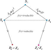
Figure 2: A pictorial form of the reduction of the discrete group $S_{5}$ to subgroups $S_{4},A_{4}$ with respect to the properties of the corresponding $\Delta_{4}$ Discriminant and the resolvent. See text for details.

As already pointed out in the introduction, guided from phenomenological reasons in this work we will analyse the ${\cal C}_{4}\times{\cal C}_{1}$ case. For this case the splitting of the five-degree polynomial is given in equation Equation (3.3) where the coefficients $a_{i}$ of the new polynomials are related to $b_{k}$ in a straightforward manner. We have already explained how these relations determine the homologies of the new coefficients from those of $b_{k}$’s and discussed their implications on the effective theory in the previous sections. However, there are additional interesting features of these coefficients with respect to the monodromy groups which we now analyse. For our case of interest, the non-trivial part is related to the fourth order polynomial so that the maximal symmetry group $S_{5}$ reduces down to $S_{4}$, (i.e. the permutation of four objects), or to some of its subgroups.

The precise determination of the Galois group depends solely on the specific structure of the coefficients $a_{n},n=1,\dots,5$. Leaving the details for the appendix, we only state here that they can be classified in terms of symmetric functions of the roots. Concerning the particular symmetry groups we are dealing with, it suffices to examine the Discriminant $\Delta_{4}$ and the resolvent of the corresponding fourth-degree polynomial.

The discriminant $\Delta_{4}$ is a symmetric function of the roots $t_{1,2,3,4}$ and as such it can always be expressed as a function of the coefficients $a_{i}$, hence $\Delta_{4}=\Delta_{4}(a_{i})$. For generic coefficients $a_{i}$ the symmetry is $S_{4}$ unless $\Delta_{4}$ can be written as a square of a quantify $\delta(a_{i})$ which is invariant under the $S_{4}$-even permutations which constitute the group $A_{4}$.

The resolvent is the cubic polynomial

$$f(x)\,=\,a_{5}^{\frac{3}{2}}(x-x_{1})(x-x_{2})(x-x_{3})\sim x^{3}+c_{1}x^{2}+c_{2}x+c_{3}$$ (4.1)

where the roots $x_{1,2,3}$ are the three $t_{i}$-combinations

$$x_{1}=t_{1}t_{2}+t_{3}t_{4},\quad{x_{2}=t_{1}t_{3}+t_{2}t_{4}},\quad{x_{3}=t_{3}t_{2}+t_{1}t_{4}}.$$ (4.2)

These are invariant under the group $D_{4}$ which is the symmetry of the square. It can be seen that all coefficients $c_{k}$ of the polynomial are symmetric functions of $t_{i}$ and therefore they can also be expressed as functions of $a_{i}$, $c_{k}(a_{i})$. Depending on the specific properties of the two quantities $\Delta_{4}$ and $f(x)$, the Galois group may be any of the $S_{5}$ subgroups depicted in figure 2.

We can readily deduce that -depending on the reducibility of the resolvent- the Galois group of the roots is either a non-Abelian or Abelian discrete group.

From the point of view of the low energy effective theory, there is a clear distinction between the two categories of discrete groups. As is well known, non-abelian discrete groups are endowed with non-trivial (non-singlet) representations. In effect, ordinary GUT representations transform non-trivially under such symmetries. This way, additional restrictions might be imposed on superpotential terms while specific forms of mass textures may arise at the same time. In the subsequent, we will focus on the particular discrete symmetry of $D_{4}$.

5 The discrete group $D_{4}$ as a Family Symmetry

In a realistic F-theory effective model a superpotential should emerge containing all necessary interaction terms. In particular it should distinguish the three families and provide correct masses to all fermion fields and at the same time should exclude all other undesired ones. In the previous sections, it has become evident that the imperative distinction of the three fermion families, in F-theory should be related to possible additional symmetries and geometric properties carried by the $SU(5)$ matter curves. In this section we will continue to explore the origin of such symmetries in the context of the ${\cal C}_{4}\times{\cal C}_{1}$ splitting. With respect to the corresponding gauge group, we may turn on suitable Abelian and non-Abelian fluxes which result in the breaking of the $SU(5)_{\perp}$ symmetry. Hence, in the present case for example one can turn on a flux along a non-trivial line bundle of the corresponding Cartan $U(1)$ so that the group originally breaks to $SU(4)_{\perp}\times U(1)_{\perp}$. Furthermore, one may assume the reduction of the $SU(4)_{\perp}$ part to some discrete group, as a consequence of a suitable non-Abelian flux or appropriate Higgsing. The case of $D_{4}\subset S_{4}$ in particular can be reached from our initial maximal symmetry of ${\cal C}_{4}$ under the following chain $SU(4)\to SU(3)\to S_{4}$. Indeed, we may invoke the one-to-one correspondence [68] of the $S_{4}$ representations to those of $SU(3)$, and decompose the $SU(4)$ ones according to the pattern shown in Table 1.

$SU(4)$	$\subset$	$SU(3)$	$\subset$	$S_{4}$
$4$	$\to$	$3+1$	$\to$	$3+1$
$6$	$\to$	$3+\bar{3}$	$\to$	$3+3$
$15$	$\to$	$8+1+3+\bar{3}$	$\to$	$3+3^{\prime}+2+1$

Table 1: The embedding of $S_{4}$ representations in the ${\cal C}_{4}$ spectral cover symmetry

An analogous symmetry reduction could be attained through the Higgs bundle description and in particular the spectral cover of the fundamental and anti-symmetric representations of our GUT gauge group. In this local picture we may exploit the fact that the geometric singularities essentially correspond to particular symmetries of the effective theory model. Hence, in accordance with the choice of the family group in our previous discussion, we will appeal to local geometry and assume the non-abelian discrete group $D_{4}$ acting on the $SU(5)_{GUT}$ representations. To study its implications in our particular construction we start by splitting the five roots $t_{i}$ into two sets

$${\cal C}_{4}\leftrightarrow\{t_{1},t_{2},t_{3},t_{4}\},\;\;\;\;{\cal C}_{1}\leftrightarrow\{t_{5}\}$$

in accordance with our choice of spectral cover splitting. Because $SU(5)_{GUT}$ representations are characterised by the weights $t_{i}$, as a result they fall into appropriate orbits. Hence, the matter curves accommodating the tenplets of $SU(5)_{GUT}$ are

$$10_{a} : \{t_{1},t_{2},t_{3},t_{4}\}$$

$$10_{b} : \{t_{5}\}$$

In the same way, if no other restrictions are imposed, the matter curves for the fiveplets of $SU(5)$ also fall into two categories

$$\bar{5}_{c} : \{t_{1}+t_{2},t_{2}+t_{3},t_{3}+t_{4},t_{4}+t_{1},t_{1}+t_{3},t_{2}+t_{4}\}$$

$$\bar{5}_{d} : \{t_{1}+t_{5},t_{2}+t_{5},t_{3}+t_{5},t_{4}+t_{5}\}.$$

We can readily observe that the orbits are ‘closed’ under the action of the elements of the $S_{4}$ group. The $SU(5)$ superpotential couplings are subject to constraints in accordance with the above classification. Hence, for example the $10_{a}10_{b}5_{d}$ coupling is allowed while $10_{a}10_{b}5_{c}$ is incompatible with the $S_{4}$ rules.

The invariance of the orbits under the action of the whole set of $S_{4}$ elements reflects the fact that the polynomial coefficients $a_{k}$ of the corresponding spectral cover fourth-order polynomial are quite generic. On the contrary, if specific restrictions are imposed on $a_{k}$ the discrete group will be a subgroup of $S_{4}$, while further splitting of the orbits will occur. We will now be more specific and consider the case of the dihedral group, $D_{4}\subset S_{4}$.

In the context of F-theory with an $SU(5)$ GUT group, if the left-over discrete group is $D_{4}$, then the four of the roots of the original $SU(5)_{\perp}$ group are permuted in accordance to the specific $D_{4}$ rules and the overall symmetry structure is:

$$E_{8}\rightarrow SU(5)_{\text{GUT}}\times SU(5)_{\perp}$$

$$\rightarrow SU(5)_{\text{GUT}}\times D_{4}\times U(1)_{\perp}\,.$$

In order to have a $D_{4}$ symmetry relating the four roots, rather than an $S_{4}$, we must appeal to Galois theory. From Table 15 in the Appendix A, we can see that this means the discriminant of the quartic part of Equation (3.3) must not be a square, while the cubic resolvent of the polynomial must be reducible.

If we assume the roots $t_{i=1,2,3,4}$, then the quartic part of Equation (3.3) has a cubic resolvent of the form given in (4.1) where the roots $x_{i}$ are the symmetric polynomials of the weights $t_{i}$ given in (4.2).

It can be shown that the discriminant ($\Delta_{f}$) of Equation (4.1) is:

$$27\Delta_{f}=4\left(a_{3}^{2}-3a_{2}a_{4}+12a_{1}a_{5}\right){}^{3}-\left(2a_{3}^{3}-9\left(a_{2}a_{4}+8a_{1}a_{5}\right)a_{3}+27\left(a_{5}a_{2}^{2}+a_{1}a_{4}^{2}\right)\right){}^{2}$$ (5.1)

which is also equal to the discriminant of the quartic polynomial relating the four roots - this is a standard property of all cubic resolvents.

By computing the coefficients as functions of the $a_{i}$ coefficients, the cubic takes the form

$$f(s)=a_{5}^{-\frac{3}{2}}[(a_{5}s)^{3}-a_{3}(a_{5}s)^{2}+(a_{2}a_{4}-4a_{1}a_{5})a_{5}s+(4a_{1}a_{3}a_{5}-a_{2}^{2}a_{5}-a_{1}a_{4}^{2})]\,.$$ (5.2)

The simplest way to make this polynomial reducible, is to demand the zero order term to vanish, $f(0)=0$. This means that one of the roots equals to zero. By setting $f(0)=0$ and using the $SU(5)$ tracelessness constraint ($b_{1}=0$) we take the following known condition [23] between the $a_{i}$’s :

$$a_{2}^{2}a_{7}=a_{1}(a_{0}a_{6}^{2}+4a_{3}a_{7})\,,$$ (5.3)

If we then substitute this into the equation for the fiveplets of the GUT group, (3.8), we get an equation factorised into 3 parts,

$$P_{5}=a_{3}(a_{2}a_{6}+4a_{1}a_{7})(a_{3}a_{6}^{2}+a_{7}(a_{2}a_{6}+a_{1}a_{7}))\,,$$ (5.4)

which indicates that we have at least 3 distinct matter curves by the usual interpretation.

$SU(5)$ Rep.	Equation	Homology
$10_{a}$	$a_{1}$	$\eta-5c_{1}-\chi$
$10_{b}$	$a_{6}$	$\chi$
$5_{a}$	$a_{3}$	$\eta-3c_{1}-\chi$
$5_{b}$	$a_{2}a_{6}+4a_{1}a_{7}$	$\eta-4c_{1}$
$5_{c}$	$a_{3}a_{6}^{2}+a_{7}(a_{2}a_{6}+a_{1}a_{7})$	$\eta-3c_{1}+\chi$

Table 2: Summary of the default matter curve splitting from spectral cover equation in the event of a $D_{4}$ symmetry accompanying an $SU(5)$ GUT group in the case of the symmetric polynomials $x_{i=1,2,3}$ as discussed in text.

The so obtained splittings of the non-trivial $SU(5)$ representations are collected in Table 2. The first column indicates the $SU(5)$ representation, while the defining equation of each corresponding matter curve is shown in column 2. In the third column we designate the associated homologies. These are readily determined from the known Chern classes of the $b_{k}$ coefficients through the equations $b_{k}=b_{k}(a_{i})$ given in (3.11), using well known procedures [12, 11]. These are expressed in terms of the known classes  $\eta,c_{1}$ and an arbitrary one designated by $\chi$.

5.1 Irreducible Representations

Thus far we have largely ignored how the group theory must be applied to matter curves in this construction. We shall now examine this side of the problem, with a particular view being taken to find the irreducible representations where possible. Given the earlier conjecture that non-Abelian fluxes can break $SU(5)_{\perp}$ to $D_{4}$, which acts as a family symmetry group in the low energy effective theory, it then follows that the low energy states must transform according to irreducible representations of $D_{4}$. In Appendix A we show how reducible 4 and 6 dimensional representations of $D_{4}$ decompose into irreducible representations. The argument in Appendix A is summarised as follows.

Knowing that we have four weights $t_{i=1,2,3,4}$, that have a relation under a $D_{4}$ symmetry, we might exploit the nature of $D_{4}$. Specifically, since $D_{4}$ can be physically interpreted as a square, we might label the corner of such a square with our weights and see how they must transform based on this. It is then clear that there should be two generators for this symmetry: a rotation about the centre by $\frac{\pi}{2}$ and a reflection along one of the lines of symmetry, which we will call $a$ and $b$ respectively. This is in keeping with the presentation of $D_{4}$:

$$a^{4}=e,\,\,\,b^{2}=e,\,\,\,bab=a^{-1}\,,$$ (5.5)

where $e$ is the identity.

It can be shown that this quadruplet of weights can be rotated into a basis with irreducible representations of $D_{4}$ - see Appendix A - by use of appropriate unitary transformations. It transpires that the irreducible basis includes a trivial singlet, a non-trivial singlet and a doublet, as summarised in Table 3. Note that we also have an extra singlet that is charged under the fifth weight ($10_{\delta}$), which must logically be a trivial singlet since it is uncharged under the $D_{4}$ symmetry.

Curve	$D_{4}$ rep.	$t_{5}$
$10_{\alpha}$	$1_{++}$	0
$10_{\beta}$	$1_{+-}$	0
$10_{\gamma}$	$2$	0
$10_{\delta}$	$1_{++}$	1

Table 3: Table summarising the representations of the tens of $SU(5)_{\text{GUT}}$

The $\bar{5}/5$ representations of the GUT group have a maximum of 10 weights before the reduction of the $SU(4)\to D_{4}$ symmetry. These have weights related to the $10$s of the GUT group: $\pm(t_{i}+t_{j})$. By consistency these must transform in the same manner as the weights of the $10$s, allowing us to unambiguously write down the generators $a$ and $b$.

By the same process as before, we may decompose this tenplet under $D_{4}$ into irreducible representations of the group. Referring to the Appendix once again, we may obtain a total of eight representations, as shown in Table 4. However, we note that three of the representations are entirely indistinguishable as they are trivial singlets with only charges under $t_{i=1,2,3,4}$.

A full decomposition of the $SU(5)_{GUT}$ representations is included in Appendix A, including the block diagonalisation procedure as applied to the singlets of the group, which will be important for model building in this work.

Curve	$D_{4}$ rep.	$t_{5}$ charge	weight relation
$\bar{5}_{\alpha}$	$1_{++}$	1	$\sum_{i=1}^{4}t_{i}$
$\bar{5}_{\beta}$	$1_{+-}$	1	$(t_{1}+t_{3})-(t_{2}+t_{4})$
$\bar{5}_{\gamma}$	$2$	1	$\left(\begin{array}[]{c}t_{1}-t_{3}\\ t_{2}-t_{4}\end{array}\right)$
$\bar{5}_{\delta}$	$1_{++}$	0	$\sum_{i=1}^{4}t_{i}$
$\bar{5}_{\epsilon}$	$1_{++}$	0	$\sum_{i=1}^{4}t_{i}$
$\bar{5}_{\zeta}$	$1_{++}$	0	$\sum_{i=1}^{4}t_{i}$
$\bar{5}_{\eta}$	$1_{+-}$	0	$(t_{1}+t_{3})-(t_{2}+t_{4})$
$\bar{5}_{\theta}$	$2$	0	$\left(\begin{array}[]{c}t_{1}-t_{3}\\ t_{2}-t_{4}\end{array}\right)$

Table 4: Table summarising the representations of the fives of $SU(5)_{\text{GUT}}$

5.2 Reconciling Interpretations

It is clear at this point that there is some tension between the two angles of attack for this problem. Obviously we must be able to describe both the non-abelian discrete group representations of the matter curves, while also being able to obtain them in some manner from the spectral cover approach. In order to achieve this, we shall attempt some form of multifurcation of the spectral cover by definition of new sections in a consistent manner.

Let us begin by defining two new sections $\kappa,\lambda$ such that

$$a_{3}\to\kappa a_{7},\;\;a_{2}\to\lambda\,a_{6}\,.$$ (5.6)

It is clear that this approach has some similarity with the tracelessness constraint solution usually employed (Equation (3.5)). Furthermore, these definitions do not generate new unwanted sections. For example, the $b_{k}$’s

$$b_{0}=-a_{0}a_{7}^{2},b_{1}=0,b_{2}=a_{7}^{2}\kappa+a_{0}a_{6}^{2},b_{3}=(\kappa+\lambda)a_{6}a_{7},b_{4}=\lambda a_{6}^{2}+a_{1}a_{7},b_{5}=a_{1}a_{6}\,,$$ (5.7)

do not acquire an overall common factor, while the discriminant

$$\Delta=108a_{0}\left(\lambda a_{6}^{2}+4a_{1}a_{7}\right)\left(\kappa^{2}a_{7}^{2}+a_{0}\left(\lambda a_{6}^{2}+4a_{1}a_{7}\right)\right){}^{2}\neq\delta^{2}$$ (5.8)

is not a square - as required for the case of a $D_{4}$ monodromy group. On the contrary, substitution to equation (3.8) gives

$$P_{a}=a_{6}^{2}\left((\kappa+\lambda)\lambda a_{7}-a_{0}a_{1}\right)$$ (5.9)

and

$$P_{b}=a_{7}\left((\kappa+\lambda)a_{6}^{2}+a_{1}a_{7}\right)\,.$$ (5.10)

This appears to generate extra matter curves by increasing the number of factors available, with the added advantage that we can easily find the homologies of our matter curves and know the flux restraints for each. We can interpret these results as a multifurcation to irreducible representations of the $D_{4}$ group.

If we further assume $a_{1}\to\mu a_{6}$, then

$$P_{b}=a_{6}a_{7}\left(a_{6}(\kappa+\lambda)+\mu a_{7}\right)\,,$$ (5.11)

and the tens of the GUT group now become:

$$P_{10}\to b_{5}=\mu\,a_{6}a_{6}\,.$$ (5.12)

So we add extra curves here as well.

Constraints	$P_{a}$	$P_{b}$	$P_{10}$
$a_{1}={\kappa a_{2}}$
$a_{3}={\lambda a_{7}}$	$a_{2}^{2}\left(a_{7}+\lambda\mu a_{7}-\alpha_{0}\kappa\mu^{2}a_{2}\right)$	$a_{2}a_{7}\left(\kappa a_{7}+(\lambda\mu+1)\mu a_{2}\right)$	$\kappa\mu a_{2}^{2}$
$a_{6}={\mu a_{2}}$

Table 5: A viable splitting option of the matter curves, respecting the constraint $\Delta\neq\delta^{2}$ as required for $D_{4}$ symmetry.

This is not a unique choice of splitting, and in fact we have a number of possible options that would be compatible with the requirement to prevent unwanted overall factors. A second option is the splitting:

$$a_{1}\to\lambda a_{2},\quad a_{3}\to\kappa a_{7}\,.$$ (5.13)

With this choice, the fives are now

$$P_{a}=a_{2}\left(a_{7}\left(a_{6}\kappa+a_{2}\right)-a_{0}a_{6}^{2}\lambda\right)$$ (5.14)

and

$$P_{b}=a_{7}\left(a_{6}^{2}\kappa+a_{2}\left(a_{7}\lambda+a_{6}\right)\right)\,.$$ (5.15)

The tens now reads $P_{10}=a_{1}a_{6}\rightarrow{\lambda a_{2}a_{6}}$.

In the same way we can find a number of combinations that leads in suitable splits. In Table 5 we show the most interesting case

$$a_{1}\to\kappa a_{2},\quad a_{3}\to\lambda a_{7},\quad\text{and}\quad a_{6}\to\mu a_{2}.$$ (5.16)

As we can see (5.16) leads in a maximal factorisation for the fives (six factors) and the tens (four factors). The homologies of the new coefficients are

$$[\kappa]=-c_{1},\quad[\mu]=-[\lambda]=4c_{1}+2\chi-\eta.$$ (5.17)

Using the above, we can calculate the homologies of the all new factors of tenplets and fives. Notice that the distribution of the the tens and the fives has be done in a arbit This case is of particular interest because we have seen that we have four tens of the GUT group, while we will also have six of the fives provided we interpret the trivial singlets as one representation. This last assumption seems reasonable given that they are otherwise indistinguishable.

5.2.1 Flux Restrictions

$P_{10}=\kappa\mu a_{2}^{2}$
Curve	factor	Homology
$10_{1}$	$\kappa$	$-c_{1}$
$10_{2}$	$a_{2}$	$\eta-4c_{1}-\chi$
$10_{3}$	$a_{2}$	$\eta-4c_{1}-\chi$
$10_{4}$	$\mu$	$-\eta+4c_{1}+2\chi$

Table 6: Distribution of the tens according to the new factorisation, $P_{10}=\kappa\mu a_{2}^{2}$.

$P_{b}=a_{2}a_{7}\left(\kappa a_{7}+(\lambda\mu+1)\mu a_{2}\right)$
Curve	$t_{5}$ charge	factor	Homology
$\bar{5}_{a}$	$1$	$a_{2}$	$\eta-4c_{1}-\chi$
$\bar{5}_{b}$	$1$	$a_{7}$	$c_{1}+\chi$
$\bar{5}_{c}$	$1$	$\kappa a_{7}+(\lambda\mu+1)\mu a_{2}$	$\chi$
$P_{a}=a_{2}^{2}\left(a_{7}+\lambda\mu a_{7}-\alpha_{0}\kappa\mu^{2}a_{2}\right)$
Curve	$t_{5}$ charge	factor	Homology
$\bar{5}_{d}$	$0$	$a_{2}$	$\eta-4c_{1}-\chi$
$\bar{5}_{e}$	$0$	$a_{2}$	$\eta-4c_{1}-\chi$
$\bar{5}_{f}$	$0$	$a_{7}+\lambda\mu a_{7}-\alpha_{0}\kappa\mu^{2}a_{2}$	$c_{1}+\chi$

Table 7: Distribution of the fives into $P_{a}$ and $P_{b}$. As we can see $P_{b}$ are related with the $t_{5}$ charge.

In order to finally marry the two understandings present in this work, we must appeal to flux restrictions. We summarise the homologies of the various matter curves in Table 6 and Table 7 with this in mind. Let us assume the usual flux restriction rules. We denote with ${\cal F}_{Y}$ the $U(1)_{Y}$ flux which breaks $SU(5)$ to the Standard Model and at the same time generates chirality to the fermions. In order to avoid a Green-Schwarz mass for the corresponding gauge boson we must require ${\cal F}_{Y}\cdot\eta={\cal F}_{Y}\cdot c_{1}=0$. For the unspecified homology $\chi$ we parametrise the corresponding flux restriction with an arbitrary integer $N={\cal F}_{Y}\cdot\chi$, hence we have the constraints:

$$\begin{gathered}{\cal F}_{Y}\cdot\chi=N,\;{\cal F}_{Y}\cdot c_{1}={\cal F}_{Y}\cdot\eta=0\,.\end{gathered}$$ (5.18)

We shall also assume the doublet-triplet splitting mechanism to be powered by this flux. Indeed, assuming $N$ units of hyperflux piercing a given matter curve, the $5$/$\bar{5}$ split according to:

$$\begin{gathered}n(3,1)_{-1/3}-n(\bar{3},1)_{+1/3}=M_{5}\,,\\ n(1,2)_{+1/2}-n(1,2)_{-1/2}=M_{5}+N\,.\end{gathered}$$ (5.19)

Thus, as long as $N\neq 0$, for the fives residing on a given matter curved the number of doublets differs from the number of triplets in the effective theory. Choosing $M_{5}=0$ for a Higgs matter curve the coloured triplet-antitriplet fields appear only in pairs which under certain conditions [2, 3] form heavy massive states. On the other hand, the difference of the doublet-antidoublet fields is non-zero and is determined solely from the hyperflux integer parameter $N$. Similarly, on a matter curve accommodating fermion generations, Equation (5.19) implies different numbers of lepton doublets and down quarks on this particular matter curve. As a consequence, the corresponding mass matrices are expected to differ.

Similarly, the $10$s decompose under the influence of $N$ hyperflux units to the following SM-representations:

$$\begin{gathered}n(3,2)_{+1/6}-n(\bar{3},2)_{-1/6}=M_{10}\,,\\ n(\bar{3},1)_{-2/3}-n(3,1)_{+2/3}=M_{10}-N\,,\\ n(1,1)_{+1}-n(1,1)_{-1}=M_{10}+N\,.\end{gathered}$$ (5.20)

Hence, as in the case of fives above, the flux effects have analogous implications on the tenplets. The first line in (5.20) in particular, generates the required up-quark chirality since for $M_{10}\neq 0$ the number of $Q=(3,2)_{1/6}$ differs from $\bar{Q}=(\bar{3},2)_{-1/6}$ representations. Moreover, from the second line it is to be observed that $N\neq 0$ leads to further splitting between the $Q=(3,2)_{1/6}$ and $u^{c}=(\bar{3},1)_{-2/3}$ multiplicities. This fact as we will see provides interesting non-trivial quark mass matrix textures.

GUT rep	Def. Eqn.	Parity:	Matter content
$10_{1}$	$\kappa$	$-$	$M_{1}Q_{L}+u^{c}_{L}M_{1}+e^{c}_{L}M_{1}$
$10_{2}$	$a_{2}$	$a$	$M_{2}Q_{L}+u^{c}_{L}(M_{2}+N)+e^{c}_{L}(M_{2}-N)$
$10_{3}$	$a_{2}$	$a$	$M_{3}Q_{L}+u^{c}_{L}(M_{3}+N)+e^{c}_{L}(M_{3}-N)$
$10_{4}$	$\mu$	$\frac{parity(a_{6})}{a}$	$M_{4}Q_{L}+u^{c}_{L}(M_{4}-2N)+e^{c}_{L}(M_{4}+2N)$
$5_{a}$	$a_{2}$	$a$	$M_{a}\bar{d}^{c}_{L}+(M_{a}-N)\bar{L}$
$5_{b}$	$a_{7}$	$b$	$M_{d}D_{u}+(M_{d}+N)H_{u}$
$5_{c}$	$\kappa a_{7}$	$-b$	$M_{c}\bar{d}^{c}_{L}+(M_{c}+N)\bar{L}$
$5_{d}$	$a_{2}$	$a$	$M_{b}\bar{D}_{d}+(M_{b}-N)\bar{H}_{d}$
$5_{e}$	$a_{2}$	$a$	$M_{e}\bar{d}^{c}_{L}+(M_{e}-N)\bar{L}$
$5_{f}$	$a_{7}$	$b$	$M_{f}\bar{d}^{c}_{L}+(M_{f}+N)\bar{L}$

Table 8: The Generalized matter spectrum for the model before marrying $D_{4}$ representations and the matter curves from the spectral cover.

6 Constructing An $N=1$ Model

Referring to the aforementioned geometric symmetry discussed at length in the Appendix, we may start out by assigning a $Z_{2}$ symmetry to our matter curves, Table LABEL:gsym. We shall demand some doublet-triplet splitting in our model, so we take the liberty of setting $N=1$, motivated by a desire to produce a spectrum free of Higgs colour triplets.

The $Z_{2}$ parity has arbitrary phases connecting the coefficients in two cycles: $a_{1,\dots,5}$ and $a_{6,7}$, which we must choose so that we can best fit the standard matter parity. The generalised parities of the matter curves are presented in Table 8. If we start with a handful of basic requirements it becomes quickly apparent how to do this and guides our assignments of the $D_{4}$ irreducible representations.

1. We must have a tree-level Top Yukawa coupling and no other tree-level Yukawas

2. We wish to forbid Dimension 4 proton decay - which may be achieved if our Higgs have $+$ parity and our matter $-$ parity

3. We want a spectrum that resembles the MSSM

If we examine Table LABEL:gsym, we can see that in order to be free from $D_{u,d}$ matter, we should choose the parity option $a=b=+$. The subtlety here is that the $H_{u}$ and $H_{d}$ must be on matter curves that have different homologies so that if we set the multiplicity for those curves to zero (preventing the $D_{u,d}$ matter), the flux naturally pushes the $H_{u}$ to be on a $5$ of the GUT group, while it pushes the $H_{d}$ to be a $\bar{5}$.

We now select our multiplicities $M_{i}$ as follows:

$$M_{2}= M_{3}=M_{b}=M_{d}=0$$

$$M_{1}= M_{a}=-M_{f}=1$$

$$M_{4}= 2$$

$$M_{c}= -4$$

This provides us with a spectrum that has only a Top Yukawa at tree-level, the correct number of matter generations, and only $u^{c}d^{c}d^{c}$ type dimension 4 parity violating operators, which should shield us from the most dangerous proton decay operators. The spectrum is summarized in Table 11.

GUT rep	Def. Eqn.	Parity	Matter content	$D_{4}$ rep.	$t_{5}$ charge
$10_{1}$	$\kappa$	$-$	$Q_{L}+u^{c}_{L}+e^{c}_{L}$	$1_{+-}$	0
$10_{2}$	$a_{2}$	$+$	$u^{c}_{L}-e^{c}_{L}$	$1_{++}$	0
$10_{3}$	$a_{2}$	$+$	$u^{c}_{L}-e^{c}_{L}$	$1_{++}$	1
$10_{4}$	$\mu$	$-$	$2Q_{L}+4e^{c}_{L}$	$2$	0
$5_{a}$	$a_{2}$	$+$	$2\bar{d}^{c}_{L}$	$2$	0
$5_{b}$	$a_{7}$	$+$	$H_{u}$	$1_{++}$	0
$5_{c}$	$\kappa a_{7}$	$-$	$-4\bar{d}^{c}_{L}-3\bar{L}$	$1_{+-}$	0
$5_{d}$	$a_{2}$	$+$	$-\bar{H}_{d}$	$1_{++}$	$-1$
$5_{e}$	$a_{2}$	$+$	$\bar{d^{c}_{L}}$	$1_{+-}$	$-1$
$5_{f}$	$a_{7}$	$+$	$-2\bar{d}^{c}_{L}$	$2$	$-1$

Table 10: Full spectrum for an $SU(5)\times D_{4}\times U(1)_{t_{5}}$ model from an F-theory construct. Note that the $-t_{5}$ charge corresponds to the $5$, while any representations that are a $\bar{5}$ will instead have $t_{5}$.

Singlet	Parity	$D_{4}$ rep.	$t_{5}$ charge	Vacuum Expectation
$\theta_{\alpha}$	$+$	$1_{++}$	$-1$	$\langle\theta_{\alpha}\rangle=\alpha$
$\theta_{\beta}$	$-$	$1_{+-}$	$-1$	$\langle\theta_{\beta}\rangle=\beta$
$\theta_{\gamma}$	$+$	$2$	$-1$	$\langle\theta_{\gamma}\rangle=(\gamma_{1},\gamma_{2})$
$\theta_{a}$	$+$	$2$	$0$	$\langle\theta_{a}\rangle=(a_{1},a_{2})$
$\nu_{r}$	$-$	$1_{+-}$	$0$	$-$
$\nu_{R}$	$-$	$2$	$0$	$-$

Table 11: Spectrum of the require singlets to construct full Yukawa matrices with the model outlined in Table 11.

6.1 Operators

Low Energy Spectrum	$D_{4}$ rep	$U(1)_{t_{5}}$	$Z_{2}$
$Q_{3},u^{c}_{3},e^{c}_{3}$	$1_{+-}$	$0$	$-$
$u^{c}_{2}$	$1_{++}$	$1$	$+$
$u^{c}_{1}$	$1_{++}$	$0$	$+$
$Q_{1,2},e^{c}_{1,2}$	$2$	$0$	$-$
$L_{i},d^{c}_{i}$	$1_{+-}$	$0$	$-$
$\nu^{c}_{3}$	$1_{+-}$	$0$	$-$
$\nu^{c}_{1,2}$	$2$	$0$	$-$
$H_{u}$	$1_{++}$	$0$	$+$
$H_{d}$	$1_{++}$	$-1$	$+$

Table 12: A summary of the low energy spectrum of the model considered. The charges include the Standard Model matter content, the $D_{4}$ family symmetry, the remaining $U(1)_{t_{5}}$ from the commutant $SU(5)$ descending from $E_{8}$ orthogonally to the GUT group, and finally the geometric $Z_{2}$ symmetry.

Models of the form presented here taken at face-value allow a large number of GUT operators, however we must ensure that all symmetries are respected. This being the case, we find that the tree-level operators found in Table 13, and constructed from the low energy spectrum summarised in Table 12, form the basis for our model, assuming the $D_{4}$ algebra rules:

$$2\times 2=1_{++}+1_{+-}+1_{-+}+1_{--}\,,$$

$$1_{a,b}\times 1_{c,d}=1_{ac,bd}\,,$$

with: $$a,b,c,d=\pm$$

As well as the expected Yukawas for the quarks and charged leptons, there are also a number of parity violating operators that could lead to dangerous and unacceptable rates of proton decay. However, provided the singlet spectrum is aligned correctly it is possible to avoid unacceptable proton decay rates via dimension 4 operators. It will not be possible to remove all parity violating operators from the spectrum though, and we will be left with $u^{c}d^{c}d^{c}$ operators that may facilitate neutron-antineutron oscillations. It is also possible to remove vector like pairs from the spectrum to insure a low energy matter content similar to the MSSM.

Operator$\to$ type	$D_{4}$ irrep.	$t_{5}$ charge	$Z_{2}$ parity
$10_{1}10_{1}5_{b}\to QUH$	$1_{++}$	$0$	$1$
$10_{1}10_{2}5_{b}\to QUH$	$1_{+-}$	$0$	$-1$
$10_{1}10_{3}5_{b}\to QUH$	$1_{+-}$	$1$	$-1$
$10_{4}10_{1}5_{b}\to QUH$	$2$	$0$	$1$
$10_{4}10_{2}5_{b}\to QUH$	$2$	$0$	$-1$
$10_{4}10_{3}5_{b}\to QUH$	$2$	$1$	$-1$
$10_{1}\bar{5}_{c}\bar{5}_{d}\to QDH$	$1_{++}$	$1$	$1$
$10_{4}\bar{5}_{c}\bar{5}_{d}\to QDH$	$2$	$1$	$1$
$10_{1}\bar{5}_{c}\bar{5}_{d}\to LEH$	$1_{++}$	$1$	$1$
$10_{4}\bar{5}_{c}\bar{5}_{d}\to LEH$	$2$	$1$	$1$
$10_{1}\bar{5}_{c}\bar{5}_{c}\to UDD$	$1_{+-}$	$0$	$-1$
$10_{2}\bar{5}_{c}\bar{5}_{c}\to UDD$	$1_{++}$	$0$	$1$
$10_{3}\bar{5}_{c}\bar{5}_{c}\to UDD$	$1_{++}$	$1$	$1$
$10_{1}\bar{5}_{c}\bar{5}_{c}\to QLD$	$1_{+-}$	$0$	$-1$
$10_{4}\bar{5}_{c}\bar{5}_{c}\to QLD$	$2$	$0$	$-1$
$10_{1}\bar{5}_{c}\bar{5}_{c}\to ELL$	$1_{+-}$	$0$	$-1$
$10_{4}\bar{5}_{c}\bar{5}_{c}\to ELL$	$2$	$0$	$-1$

Table 13: List of all trilinear couplings available in the $\text{SU}(5)\times D_{4}\times U(1)$ model presented. At tree-level, these operators are not all immediately allowed, since the $D_{4}$ and $t_{5}$ symmetries must be respected.

6.1.1 Quark sector

The up-type quarks have four operators which contribute to the Yukawa matrix. Firstly, we have a tree level top quark coming from the operator $10_{1}10_{1}5_{b}$, which is the only tree level Yukawa operator found in the Quark and Charged Lepton sectors. The remaining three operators are non-renormalisable operators subject to suppression. We shall assume that the up-type Higgs gets a vacuum expectation value, $\langle H_{u}\rangle=v_{u}$. The singlets involved must have vacuum expectation values as summarised in Table 11. The following mass terms are generated

$$10_{1}10_{1}5_{b} \rightarrow y_{1}v_{u}Q_{3}u_{3}^{c}$$

$$10_{4}10_{1}5_{b}\theta_{a} \rightarrow y_{2}v_{u}(Q_{2}a_{2}+Q_{1}a_{1})u_{3}^{c}$$

$$10_{4}10_{3}5_{b}\theta_{a}\theta_{\beta} \rightarrow y_{3}v_{u}\beta(Q_{2}a_{2}+Q_{1}a_{1})u_{2}^{c}$$

$$10_{1}10_{3}5_{b}\theta_{\beta} \rightarrow y_{4}v_{u}\beta Q_{3}u^{c}_{2}$$

giving rise to the up-quark mass texture

$$M_{u,c,t} =v_{u}\left(\begin{array}[]{ccc}0&y_{3}a_{1}\beta&y_{2}a_{1}\\ 0&y_{3}a_{2}\beta&y_{2}a_{2}\\ 0&y_{4}\beta&y_{1}\end{array}\right).$$

The lightest generation does not get an explicit mass from this mechanism, but we can expect a small correction to come from non-commutative fluxes or instantons [38, 40, 43], thus generating a small mass for the first generation.

The down-type quarks contribute a further two operators to the model. These will be symmetric across the righthanded $d^{c}$ since all three generations are found on the $5_{c}$ matter curve. We once again assume the Higgs to get a vacuum expectation, $\langle H_{d}\rangle=v_{d}$. As before, we also give the singlets a vacuum expectation value: $\langle\theta_{\alpha}\rangle=\alpha$ and $\langle\theta_{\gamma}\rangle=(\gamma_{1},\gamma_{2})^{T}$. As a result, we get the Yukawa contributions

$$10_{1}\bar{5}_{c}\bar{5}_{d}\theta_{\alpha} \rightarrow y_{4,i}v_{d}Q_{3}d_{i}^{c}\alpha$$

$$10_{4}\bar{5}_{c}\bar{5}_{d}\theta_{\gamma} \rightarrow y_{5,i}v_{d}(Q_{2}\gamma_{2}+Q_{1}\gamma_{1})d_{i}^{c}$$

and consequently, the down quark mass matrix form

$$M_{d,s,b} =v_{d}\left(\begin{array}[]{ccc}y_{5,1}\gamma_{1}&y_{5,2}\gamma_{1}&y_{5,3}\gamma_{1}\\ y_{5,1}\gamma_{2}&y_{5,2}\gamma_{2}&y_{5,3}\gamma_{2}\\ y_{4,1}\alpha&y_{4,2}\alpha&y_{4,3}\alpha\end{array}\right).$$

However, this mass matrix will be subject to the rank theorem, requiring that there be some suppression factor between the copies of the operator, which we indicate by the second index, $y_{i,j}$.

6.1.2 Charged Leptons

The Charged Lepton Yukawas are determined by the same operators as the Down-type quarks, subject to a transpose. As such their mass matrix is as follows:

$$10_{1}\bar{5}_{c}\bar{5}_{d}\theta_{\alpha} \rightarrow y_{6,i}v_{d}L_{i}e_{3}^{c}\alpha$$

$$10_{4}\bar{5}_{c}\bar{5}_{d}\theta_{\gamma} \rightarrow y_{7,i}v_{d}L_{i}(e^{c}_{2}\gamma_{2}+e^{c}_{1}\gamma_{1})$$

$$M_{e,\mu,\tau} =v_{d}\left(\begin{array}[]{ccc}y_{7,1}\gamma_{1}&y_{7,1}\gamma_{2}&y_{6,1}\alpha\\ y_{7,2}\gamma_{1}&y_{7,2}\gamma_{2}&y_{6,2}\alpha\\ y_{7,3}\gamma_{1}&y_{7,3}\gamma_{2}&y_{6,3}\alpha\end{array}\right).$$

The mass relations between charged leptons and down-type quarks will not be constrained to be exact as the operators can be assumed to be localized to different parts of the GUT surface. Once again this is subject to the rank theorem, but will be able to produce a light first generation through other mechanisms.

6.1.3 Neutrinos

Over the coming years, all three lepton mixing angles are expected to be measured with increasing precision. A first tentative hint for a value of the CP-violating phase $\delta_{CP}\sim-\pi/2$ has also been reported in global fits [63, 64, 65]. However the mass squared ordering (normal or inverted), the scale (mass of the lightest neutrino) and nature (Dirac or Majorana) of neutrino mass so far all remain unknown.

On the theory side, there are many possibilities for the origin of light neutrino masses $m_{i}$ and mixing angles $\theta_{ij}$. Perhaps the simplest and most elegant idea is the classical see-saw mechanism, in which the observed smallness of neutrino masses is due to the heaviness of right-handed Majorana neutrinos [66],

$$m^{\nu}=-m^{D}M^{-1}_{R}(m^{D})^{T},$$ (6.1)

where $m^{\nu}$ is the light effective left-handed Majorana neutrino mass matrix (i.e. the physical neutrino mass matrix), $m^{D}$ is the Dirac mass matrix (in LR convention) and $M_{R}$ is the (heavy) Majorana mass matrix. Although the see-saw mechanism generally predicts Majorana neutrinos, it does not predict the “mass hierarchy”, nor does it yield any understanding of lepton mixing. In order to overcome these deficiencies, the see-saw mechanism must be supplemented by other ingredients. In order to obtain sharp predictions for lepton mixing angles, the relevant Yukawa coupling ratios need to be fixed, for example using vacuum alignment of family symmetry breaking flavons (for reviews see e.g. [57, 58, 59, 60]).

In F-theory, neutrinos may admit both Dirac and Majorana mass terms. As such, we would like to use the see-saw mechanism to achieve small neutrino masses via a GUT scale Majorana type mass. Any Dirac type mass comes from an operator of the form $m_{D}\sim\theta_{\nu}5_{b}\bar{5}_{c}$, while the right-handed Majorana mass terms are of the form $M\theta_{\nu}\theta_{\nu}$. Although we have a non-Abelian $D_{4}$ family symmetry, the lepton doublets $L$ are in singlet representations (see Table 12), so the model offers no opportunity to make predictions for the lepton mixing angles.

The singlet representations and parities, as detailed in the Appendix A and B, allow us up to nine singlets in this model. Let us then match our right-handed neutrinos to the representations $1_{+-}$ and a doublet, as allowed from our spectrum. This will then give the operators for the Dirac mass:

$$\theta_{\nu_{r}}5_{b}\bar{5}_{c} \rightarrow y_{8,i}v_{u}\nu^{c}_{3}L_{i}$$

$$\theta_{\nu_{R}}5_{b}\bar{5}_{c}\theta_{a} \rightarrow y_{9,i}v_{u}(\nu^{c}_{1}a_{1}+\nu^{c}_{2}a_{2})L_{i}$$

$$m_{D} =v_{u}\left(\begin{array}[]{ccc}y_{9,1}a_{1}&y_{9,1}a_{2}&y_{8,1}\\ y_{9,2}a_{1}&y_{9,2}a_{2}&y_{8,2}\\ y_{9,3}a_{1}&y_{9,3}a_{2}&y_{8,3}\end{array}\right).$$

This Dirac matrix can be shown to be rank two, which will cause our lightest neutrino to be massless. While this is not explicitly ruled out by experiment, a small mass can be generated through some higher order operators from other singlets in the spectrum if required - for example a singlet of the type $1_{--}$ with $+$ parity. This will allow an explicit Dirac type mass, however similar analysis has been done elsewhere ( for example [24]), so we omit in depth discussion here.

The Majorana terms corresponding to this choice of neutrino spectrum are simply calculated, as one might expect:

$$\theta_{\nu_{r}}\theta_{\nu_{r}} \rightarrow m\nu^{c}_{3}\nu^{c}_{3}$$

$$\theta_{\nu_{R}}\theta_{\nu_{R}} \rightarrow M\nu^{c}_{1}\nu^{c}_{2}$$

$$\theta_{\nu_{r}}\theta_{\nu_{R}}\theta_{a} \rightarrow y\nu^{c}_{3}\nu^{c}_{2}a_{2}+y\nu^{c}_{3}\nu^{c}_{1}a_{1}$$

$$M_{R} =\left(\begin{array}[]{ccc}0&M&ya_{1}\\ M&0&ya_{2}\\ ya_{1}&ya_{2}&m\end{array}\right).$$

This may also be allowed corrections via extra singlets, though it will not be needed for this work.

The effective neutrino mass can be calculated from the seesaw mechanism via $m_{\nu}=-m_{D}M_{R}^{-1}m_{D}^{T}$. The resulting mass matrix appears complicated, with elements given in full as:

$$m_{11}= M{y_{8,1}}^{2}+2{a_{1}}{a_{2}}{y_{9,1}}({m}{y_{9,1}}-2{y_{8,1}}y)$$

$$m_{12}=m_{21}= M{y_{8,1}}{y_{8,2}}-2{a_{1}}{a_{2}}({y_{8,2}}y{y_{9,1}}-{m}{y_{9,2}}{y_{9,1}}+{y_{8,1}}y{y_{9,2}})$$

$$m_{13}=m_{31}= M{y_{8,1}}{y_{8,3}}-2{a_{1}}{a_{2}}({y_{8,3}}y{y_{9,1}}-{m}{y_{9,3}}{y_{9,1}}+{y_{8,1}}y{y_{9,3}})$$

$$m_{22}= M{y_{8,2}}^{2}+2{a_{1}}{a_{2}}{y_{9,2}}({m}{y_{9,2}}-2{y_{8,2}}y)$$

$$m_{23}=m_{32}= M{y_{8,2}}{y_{8,3}}-2{a_{1}}{a_{2}}({y_{8,3}}y{y_{9,2}}-{m}{y_{9,3}}{y_{9,2}}+{y_{8,2}}y{y_{9,3}})$$

$$m_{33}= M{y_{8,3}}^{2}+2{a_{1}}{a_{2}}{y_{9,3}}({m}{y_{9,3}}-2{y_{8,3}}y)$$

with an overall scaling of $m_{0}=v_{u}^{2}({M{m}-2{a_{1}}{a_{2}}y^{2}})^{-1}$.

In order to extract mixing parameters and mass scales, we will parameterize the matrix in the following way:

$$X_{i}= \frac{y_{8,i}}{y_{8,1}},\;Z_{i}=\frac{y_{9,i}}{y_{8,1}},\;G=\frac{2a_{1}a_{2}}{M}$$ (6.2)

with $i=1,2,3$, and trivially $X_{1}=1$. Note that $X_{2,3}$ and $Z_{j}$ are not required to be order one due to the parametrization choice. Let us go a step further, approximating $m\approx M$ and setting $Z_{3}=0$, then the mass matrix is given by:

where:

$$m_{0}=\frac{v_{u}^{2}Mx_{1}^{2}}{M^{2}-Gy^{2}}\,.$$ (6.4)

This parametrization allows for comparatively straightforward extraction of mixing parameters. Using Mathematica, we fit the Ratio of mass squared differences in this model to experimental constraints, allowing us to extract a mass scale for the neutrinos while fitting parameters to allow acceptable mixing angles.

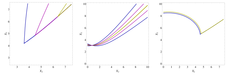
Figure 3: Left: Plot of $\sin^{2}{\theta_{12}}$ across its $3\sigma$ range (blue-0.270, pink-0.304, yellow-0.344), Center: Plot of $\sin^{2}{\theta_{23}}$ across its $3\sigma$ range (blue-0.382, pink-0.452, yellow-0.5). Note that the upper bound of $\sin^{2}{\theta_{23}}$ is $0.643$, but this is not allowed by the model, which permits a maximum of 0.5 for these parameters. Right: Plot of the mass squared difference ratio, R, for its upper and lower bounds of 31.34 (blue) and 34.16 (yellow). For all three plots the parameter space $(X_{2},X_{3})$ is plotted since these terms should lead the mixing. The remaining parameters are set at values that yield consistent mixing parameters: $(Z_{1}\approx 2.4,Z_{2}\approx 4.1,G\approx 0.6,y\approx 0.3)$.

Figure 3 shows plots of the $3\sigma$ ranges of $\sin^{2}{\theta_{12}}$, $\sin^{2}{\theta_{23}}$ and $R=\left|\frac{m_{3}^{2}-m_{2}^{2}}{m_{2}^{2}-m_{1}^{2}}\right|$ in the parameter space of $(X_{2},X_{3})$. This shows that while there are some sharp cutoffs in the parameter space, the key variables can still be allowed. A full simulation of parameters gives, for example:

Inputs: $$\left(X_{2}=4.5,\,X_{3}=5.7,\,Z_{1}=2.4,\,Z_{2}=4.1,\,G=0.6,\,y=0.3\right)$$

Outputs: $$\left(R=33.2,\,\theta_{12}=32.4,\,\theta_{13}=9.07,\,\theta_{23}=39.2\right)$$

This also allows us to extract the neutrino masses using the mass differences, which are an implicit input parameter used in calculation of R. We know from the Dirac matrix rank that at this order of operator one neutrino is massless, so then the remaining two masses are (within experimental errors) equal to the square root of the mass differences:

$$m_{1}=0\ \text{meV}\,,\,m_{2}=8.66\ \text{meV}\,,\,m_{3}=50.3\ \text{meV}\,.$$ (6.5)

Being at the absolute minimum scale for the neutrino masses, this is automatically compatible with cosmological constraints.

6.2 $\mu$-Terms

In this set-up the standard Higgs sector $\mu$-term requires coupling to a singlet in order to cancel the charges under $U(1)_{t_{5}}$. The most suitable coupling allowed by the singlet sector is a term of the type:

$$\lambda_{1}\theta_{\alpha}H_{u}H_{d}\,.$$ (6.6)

As such the $\mu$ term is proportional to the vacuum expectation of the singlet $\theta_{\alpha}$:

$$\mu=\lambda_{1}\langle\theta_{\alpha}\rangle$$ (6.7)

Since this singlet couples to the Charged Lepton and the Bottoms quark Yukawa matrices, the resulting vacuum expectation should allow a TeV scale $\mu$-term while not affecting these Yukawas too strongly. Note that since the operators in the Charged Lepton and Bottom quark sectors are non-renormalisable, the coupling should be suppressed by a large mass scale, making this possible. It is also shown in the D-flatness conditions (provided in the appendix) that we have a deal of freedom when choosing the vacuum expectation value for $\theta_{\alpha}$.

A second term of the type:

$$\lambda_{2}\theta_{a}\theta_{\gamma}H_{u}H_{d}\,$$ (6.8)

will also contribute to the $\mu$ terms, which is non-renormalisable and should be suppressed by some large mass scale. Refering to the F-flatness conditions and a cursory calculation of this coupling, we see that this contributes proportionally to the product of the vacuum expectations of the $\theta_{a}$ and $\theta_{\gamma}$ singlets. This again seems acceptable.

7 Baryon number violation

7.1 Proton decay

It is well known that in the absence of particular types of symmetries such as R-parity, the MSSM as well as ordinary GUT symmetries are not adequate to ban rare processes leading to baryon and/or lepton number violation. Moreover, specific $SU(5)$ GUT representations include additional states leading to similar drawbacks. Such states are the Higgs colour triplets being components of the very same fives containing the up and down SM Higgs doublets. If both Higgs fields localise on the same matter curve they generate graphs contributing to proton decay from effective operators of the form $M_{GUT}^{-1}\,QQQL$. Since their Yukawa couplings are expected to be of order one, the suppression factor $M_{GUT}^{-1}$ is not sufficient to reduce baryon number violating processes to acceptable rates.

In F-theory it is possible to turn on suitable fluxes so that the Higgs triplets are removed from the low energy spectrum. However even in this case their associated Kaluza-Klein modes generate the same type of non-renormalisable terms where now the suppression factor is replaced by the KK scale $M_{KK}^{-1}$. Since the $M_{KK}$ mass scale is not expected to be substantially larger that the $M_{GUT}$ scale, one would not expect a significant suppression of these operators. It is possible to achieve further suppression however, if the parts of the colour triplet-antitriplet pair emerge from different matter curves so that a direct tree-level mass term is not generated.

In practice, the realistic constructions are more complicated and the whole issue of baryon and lepton number violation is more involved. Firstly, as we have analysed in Section 3.4, the role of R-parity in this work is played by a $Z_{2}$ symmetry of geometric origin which does not necessarily coincide with the standard R-parity imposed in field theory supersymmetric models. Secondly, accompanying symmetries emerging from the $SU(5)_{\perp}$ breaking affix additional quantum numbers to the GUT representations and as such, they imply further restrictions on the superpotential of the effective theory.

We pursue our investigation, elaborating the above for the present model. Clearly, in order to establish the existence of a proton decay operator, we should pay heed to many more factors than in ordinary field theory GUTs, such as accompanying symmetries, geometric properties and flux effects. In the present model, there is a combination of constraints associated to the $D_{4}$ group, the $Z_{2}$ discrete symmetry of geometric origin as well as a $U(1)$ factor that should be respected. Although these symmetries eliminate a singificant number of catastrophic operators, yet there remain trilinear terms which are potentially dangerous, which we now discuss. We start with the trilinear couplings, which take two forms,

$$10\cdot\bar{5}\cdot\bar{5} \to Qd^{c}H_{d}+QD^{c}L+e^{c}LH_{d}+u^{c}d^{c}d^{c}$$ (7.1)

$$10\cdot 10\cdot 5 \to Qu^{c}H_{u}+u^{c}e^{c}D^{c}+QQD^{c}$$ (7.2)

which in principle, give rise to dimension 5 proton decay provided the following coupling exists for the Higgs colour triplet:

$$\Phi 5\bar{5}\to\langle\Phi\rangle D\,D^{c}$$ (7.3)

where $\Phi$ a suitable singlet field acquiring a non-zero vev. However, our flux choice eliminates the coloured triplets from Higgs fields (see Table 11) and as a result such terms do not exist.

In addition to the above type of operators, there are trilinear R-parity violating terms that give rise to proton decay through similar graphs. Checking Table 13 one can see that there is a potentially dangerous baryon violating term, namely

$$10_{2}\bar{5}_{c}\bar{5}_{c}$$ (7.4)

giving rise to a $u^{c}d^{c}d^{c}$ operator (because of flux effects $10_{2}$ does not contain $Q$, hence the operator $Qd^{c}L$ does not exist). Thus, (7.4) contributes to proton decay only if analogous dimension-four operators from terms of the type $10_{i}10_{j}5_{k}$ are simultaneously present in the superpotential. In the present model such terms do not exist, hence proton stability is ensured. Nevertheless, there are other interesting implications of the above operator that could be the low energy imprint of the present model, which we will now discuss.

7.2 Neutron-Antineutron oscillations

As mention in the previous section, the model presented is free from proton decay at the lowest orders. However, it is subject to operators which are classically considered to be parity violating. Since these operators are all of the type $u^{c}d^{c}d^{c}$, they will instead facilitate neutron-antineutron oscillations. While this is a seldom considered property of GUT models, work has been done to calculate transmission amplitudes of such processes by Mohapatra and Marshak [67] and later on by Goity and Sher [69] among others. The contributions to the process are generated from tree-level and box type graphs (see [69], the reviews [70, 71] and references therein), with typical cases shown in Figure 4.

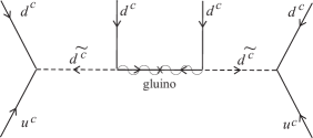
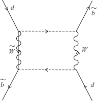
Figure 4: Feynman graphs for $n-\bar{n}$ oscillation processes. Top: oscillation via a gluino, Bottom: box-graph process.

In the paper of Goity and Sher, they argue that one can identify a competitive mechanism, with a fully calculable transition amplitude, which sets a bound on $\lambda_{dbu}$. This mechanism is based on the sequence of reactions $u_{R}d_{R}+d_{L}\rightarrow\tilde{b}_{R}^{*}+d_{L}\rightarrow{(\tilde{b}_{L}^{*}+d_{L}\rightarrow{\bar{d}_{L}+\tilde{b}_{L}})}\rightarrow{\bar{d}_{L}+\bar{u}_{R}\bar{d}_{R}}$, where the intermediate transition in the parentheses, $\tilde{b}_{L}^{*}+d_{L}\rightarrow{\bar{d}_{L}+\tilde{b}_{L}}$, is due to a W boson and gaugino exchange box diagram . The choice of intermediate bottom squarks is the most favourable one in order to maximise factors such as $m_{b}^{2}/m_{W}^{2}$, which arise from the electroweak interactions of d-quarks in the box diagram (Figure 3).

Calculation of the diagram gives the following relation for the decay rate,

$$\Gamma=-\frac{3g^{4}\lambda^{2}_{dbu}M_{\tilde{b}_{LR}}^{2}m_{\tilde{w}}}{8\pi^{2}M_{\tilde{b}_{L}}^{4}M_{\tilde{b}_{R}}^{4}}|\psi(0)|^{2}\sum_{j,j^{\prime}}^{u,c,t}\xi_{jj^{\prime}}J(M_{\tilde{w}}^{2},M_{W}^{2},M_{u_{j}}^{2},M_{\tilde{u}_{j^{\prime}}}^{2})$$ (7.5)

where the mass term $M_{\tilde{b}_{LR}}$, which mixes $\tilde{b}_{L}$ and $\tilde{b}_{R}$, is given by $M_{\tilde{b}_{LR}}=Am_{b}$. Here $A$ is the soft SUSY breaking parameter with $A=m_{\tilde{w}}=200GeV$, and $\xi_{jj^{\prime}}$ is a combination of CKM matrix parameters,

$$\xi_{jj^{\prime}}=V_{bu_{j}}V_{u_{j}d}^{\dagger}V_{bu_{j^{\prime}}}V_{u_{j^{\prime}}d}^{\dagger}\,$$ (7.6)

and the $J$ functions are given by:

$$J(m_{1},m_{2},m_{3},m_{4})=\sum_{i=1}^{4}\frac{m_{i}^{4}\ln(m_{i}^{2})}{\prod_{k\neq{i}}(m_{i}^{2}-m_{k}^{2})}\,.$$ (7.7)

The $n$-$\bar{n}$ oscillation time is $\tau=1/\Gamma$ and the current experimental limits gives, $\tau\gtrsim{10^{8}sec.}$ [70]. Finally $|\psi(0)|$ is the baryonic wave function matrix element for three quarks inside a nucleon. This parameter was calculated to be $|\psi(0)|^{2}=10^{-4}$ and $0.8\times{10^{-4}}GeV^{-6}$ in MIT Bag models. From the experimental limit on the neutron oscillation time we can obtain the bound on $\lambda_{dbu}$. The results depend on CKM parameters and the squarks masses. In Figure 5 we reproduce the results of Goity and Sher. As we can see the upper bound on $\lambda_{dbu}$ is between 0.005 and 0.1.

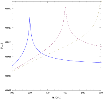
Figure 5: Goity and Sher bounds on $\lambda_{dbu}$. They assumed that up and bottom squark masses are degenerate. Blue: $M_{\tilde{u}}=M_{\tilde{c}}=200GeV$, Dashed: $M_{\tilde{u}}=M_{\tilde{c}}=400GeV$, Dotted: $M_{\tilde{u}}=M_{\tilde{c}}=600GeV$. Also we took $M_{\tilde{b}_{L}}=M_{\tilde{b}_{R}}=350GeV$. The peaks corresponds to GIM mechanism effects.

Next we use the Equation (7.5) to recalculate the bounds on $\lambda_{dbu}$ with the latest experimental results for the SUSY mass parameters. In Figure 6 the curves correspond to squark masses of 800, 1000 and 1200GeV (Blue, dashed and dotted accordingly). As we can see the value of $\lambda_{dbu}$ lies between 0.1 and $\sim$ 0.5 for stop mass between 500 and 1600GeV, neglecting GIM effects.

In F-theory there is an associated wavefunction [34]-[41] to the state residing on each matter curve and it can be determined by solving the corresponding equations of motion [2]. The solutions show that each wavefunction is peaked along the corresponding matter curve. Yukawa couplings are formed at the point of intersection of three matter curves where the corresponding wavefunctions overlap. To estimate the corresponding Yukawa coupling we need to perform an integration over the three overlapping wavefunctions of the corresponding states participating in the trilinear coupling. Taking into account mixing effects this particular coupling is estimated to be of the order $\lambda_{dbu}\leq 10^{-1}$. From the figure it can be observed that recent $n-\bar{n}$ oscillation bounds on $\lambda_{dbu}$ are compatible with such values.

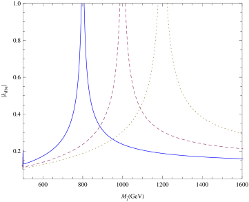
Figure 6: New bounds on $\lambda_{dbu}$ using the latest experimental limits. Blue: $M_{\tilde{u}}=M_{\tilde{c}}=800GeV$, Dashed: $M_{\tilde{u}}=M_{\tilde{c}}=1000GeV$, Dotted: $M_{\tilde{u}}=M_{\tilde{c}}=1200GeV$. Also we use the following values for the other parameters: $M_{\tilde{b}_{L}}=M_{\tilde{b}_{R}}=500GeV$, $\tau=10^{8}sec.$ and $|\psi(0)|=0.9\times{10^{-4}}GeV^{-6}$.

8 Conclusions

In this work an F-theory derived $SU(5)$ model was constructed, with the implications of the arising non-Abelian familiy symmetry being considered, following from work in [23] and [24]. Using the spectral cover formalism, assuming a point of $E_{8}$ enhancement descending to an $SU(5)$ GUT group, the corresponding maximal symmetry (also $SU(5)$) should reduce down to a subgroup of the Weyl group, $S_{5}$. In this paper we derive the conditions on the spectral cover equation in the case of the non-abelian discrete group $D_{4}$, which was assumed to play the role of a family symmetry. A novel geometric symmetry was also employed to produce an R-parity-like $Z_{2}$ symmetry. The combined effect of this framework on the effective field theory has been examined, and the resulting model shown to exhibit parity violation in the form of neutron-antineutron oscillations, while being free from dangerous proton decay operators. The experimental constraints on this interesting process have been calculated, using current data on the masses of supersymmetric partners. Detection of such baryon-violating processes, without proton decay, serve as a potential smoking gun for this type of model.

The physics of the neutrino was also considered, and it was shown that at lowest orders this model predicts a massless first generation neutrino. Correspondingly, the masses of the two other generations then equate to the mass differences from experiment, with the hierarchy being normal ordered. The mixing angles were also probed numerically, with results that are consistent with large mixing in the neutrino sector and a non-zero reactor mixing angle.

In conclusion F-theory model building predicts in a natural way the coexistence of GUT models with non-Abelian discrete symmetry extensions. The reach symmetry content following from the decomposition of the $E_{8}$ covering group and the geometric symmetries emerging from the internal manifold structure are sufficient to incorporate successful non-Abelian groups which have already been proposed in phenomenological constructions during the last decade. The distinct role of the discrete groups as family symmetries occurs naturally in the F-theory constructions. Moreover, the theory provides powerful tools to get an effective field theory with definite predictions.

9 Acknowledgments

SFK acknowledges partial support from the European Union FP7 ITN INVISIBLES (Marie Curie Actions, PITN- GA-2011- 289442). AM is supported by an STFC studentship. GKL acknowledges partial support from the European Union (European Social Fund - ESF) and Greek national funds through the Operational Program “Education and Lifelong Learning” of the National Strategic Reference Framework (NSRF) - Research Funding Program: “ARISTEIA”. Investing in the society of knowledge through the European Social Fund.

Appendix A Irreducible representations of $D_{4}$

Since we have four weights related, the representation of the 10s of the GUT group will be quadruplets of $D_{4}$: $(t_{1},t_{2},t_{3},t_{4})^{\text{T}}$. Physically we may take each of these weights to represent a corner of a square (or an equivalent interpretation). These weights will transform in this representation such that the two generators required to describe all possible transformations are equivalent to a rotation about the center of the square of $\frac{\pi}{2}$ and a reflection about a line passing through the center - say the diagonal running between the top right and bottom left corners (see Figure 7).

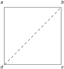
Figure 7: A physical representation of the symmetry group $D_{4}$. The dashed line shows a possible reflection symmetry, while it also has a rotational symmetry if rotated by $\frac{n\pi}{2}$.

The two generators are:

$$a= \left(\begin{array}[]{cccc}0&0&0&1\\ 1&0&0&0\\ 0&1&0&0\\ 0&0&1&0\end{array}\right)\,,$$ (A.5)

$$b= \left(\begin{array}[]{cccc}1&0&0&0\\ 0&0&0&1\\ 0&0&1&0\\ 0&1&0&0\end{array}\right)\,.$$ (A.10)

These generators must obey the general conditions for dihedral groups, which for $D_{4}$ are:

$$a^{4}=b^{2}=$$ I (A.11)

$$b\cdot a\cdot b= a^{-1}$$ (A.12)

It is trivial to see that these conditions are obeyed by our generators. In order to obtain the irreducible representations we should put this basis into block-diagonal form, which is achieved by applying the appropriate unitary matrices.

Since $D_{4}$ is known to have a two-dimensional irreducible representation, we might assume that our four-dimensional case can be taken to a block diagonal form including either a doublet and two singlets or two doublets via a unitary transformation.

If we initially assume two doublets, then we may put some conditions on our unitary matrix:

$$A^{\prime}= U\cdot A\cdot U^{\text{T}}=\left(\begin{array}[]{cccc}-&-&0&0\\ -&-&0&0\\ 0&0&-&-\\ 0&0&-&-\end{array}\right)$$ (A.17)

$$B^{\prime}= U\cdot B\cdot U^{\text{T}}=\left(\begin{array}[]{cccc}-&-&0&0\\ -&-&0&0\\ 0&0&-&-\\ 0&0&-&-\end{array}\right)$$ (A.22)

$$\text{I}= U\cdot U^{\text{T}}\,.$$ (A.23)

If we make use of these conditions, there are a number of equivalent solutions for $U$, one of which is:

$$U=\frac{1}{\sqrt{2}}\left(\begin{array}[]{cccc}1&0&1&0\\ 0&1&0&1\\ 1&0&-1&0\\ 0&1&0&-1\end{array}\right)\,.$$ (A.24)

This matrix will give a block diagonal form for the generators. Explicitly this is:

$$A^{\prime}= \left(\begin{array}[]{cccc}0&1&0&0\\ 1&0&0&0\\ 0&0&0&-1\\ 0&0&1&0\end{array}\right)\,,$$ (A.29)

$$B^{\prime}= \left(\begin{array}[]{cccc}1&0&0&0\\ 0&1&0&0\\ 0&0&1&0\\ 0&0&0&-1\end{array}\right)\,,$$ (A.34)

$$\left(\begin{array}[]{c}t_{1}\\ t_{2}\\ t_{3}\\ t_{4}\end{array}\right) \rightarrow\frac{1}{\sqrt{2}}\left(\begin{array}[]{c}t_{1}+t_{3}\\ t_{2}+t_{4}\\ t_{1}-t_{3}\\ t_{2}-t_{4}\end{array}\right)\,.$$ (A.43)

A cursory examination reveals that the conditions for $D_{4}$ are still fulfilled by this new basis, and it would seem that at a minimum we have two doublets of the group. However we shall now examine if one of the doublets decomposes to two singlets.

The upper block of the $B^{\prime}$ generator takes the form of the identity, so we might suppose that the first of our two doublets could decompose into two singlets. Using the same conditions as for the four-dimensional starting point, which can be enforced on the two-dimensional case, we can find easily that:

$$V= \frac{1}{\sqrt{2}}\left(\begin{array}[]{cc}1&1\\ 1&-1\end{array}\right)$$ (A.46)

$$A^{\prime\prime}= \left(\begin{array}[]{cc}1&0\\ 0&-1\end{array}\right)$$ (A.49)

$$B^{\prime\prime}= \left(\begin{array}[]{cc}1&0\\ 0&1\end{array}\right)$$ (A.52)

$$\frac{1}{\sqrt{2}}\left(\begin{array}[]{c}t_{1}+t_{3}\\ t_{2}+t_{4}\end{array}\right) \rightarrow\frac{1}{2}\left(\begin{array}[]{c}t_{1}+t_{2}+t_{3}+t_{4}\\ t_{1}-t_{2}+t_{3}-t_{4}\end{array}\right)$$ (A.57)

It would seem then in this case that the four-dimensional representation of $D_{4}$ can be reduced to a doublet and two singlets forming an irreducible representation. The type of the singlets can be determined by examination of the conjugacy classes of the group, which reveals that the upper singlet is of the type $1_{++}$, while the lower is $1_{+-}$. Table 2 summarising the representations of the tens.

A.1 $D_{4}$ representations for GUT group Fundamental representation

The roots of the five-curves can also be described in terms of the roots:

$$t_{i}+t_{j}=0\,\forall i\neq j\,.$$ (A.58)

which gives a total of ten solutions, though these will be related by the discrete group. Under the $D_{4}$ symmetry, we can see trivially that since the weight $t_{5}$ is chosen to be the invariant root, all the roots corresponding to the fives of the form $t_{i}+t_{5}$ will transform separately to the $i,j\neq 5$ roots. In fact, these will form a doublet and two singlets: $1_{++}$ and $1_{+-}$.

The remaining six roots of $P_{5}$ can be constructed into a sextet:

$$R_{6}=\left(\begin{array}[]{c}t_{1}+t_{3}\\ t_{2}+t_{4}\\ t_{1}+t_{2}\\ t_{3}+t_{4}\\ t_{1}+t_{4}\\ t_{2}+t_{3}\end{array}\right)\,.$$ (A.59)

By construction, we have arranged that the array manifestly has block diagonal generators, $A$ and $B$, such that the first two lines have generators:

$$A=\left(\begin{array}[]{cc}0&1\\ 1&0\end{array}\right)\,\,\,B=\left(\begin{array}[]{cc}1&0\\ 0&1\end{array}\right)\,.$$ (A.60)

We can again refer to the previous results to see that this reduces to two singlets: $1_{++}$ and $1_{+-}$.

The remaining quadruplet has generators:

$$A=\left(\begin{array}[]{cccc}0&0&1&0\\ 0&0&0&1\\ 0&1&0&0\\ 1&0&0&0\end{array}\right)\,\,\,B=\left(\begin{array}[]{cccc}0&0&0&1\\ 0&0&1&0\\ 0&1&0&0\\ 1&0&0&0\end{array}\right)\,,$$ (A.61)

which we can block diagonalise using the unitary matrix:

$$U=\frac{1}{\sqrt{2}}\left(\begin{array}[]{cccc}1&1&0&0\\ 0&0&1&1\\ -1&1&0&0\\ 0&0&1&-1\\ \end{array}\right)\,.$$ (A.62)

This gives two blocks, which are distiniguished principally by their $A$ generators:

$$A^{\prime}=\left(\begin{array}[]{cccc}0&1&0&0\\ 1&0&0&0\\ 0&0&0&-1\\ 0&0&1&0\\ \end{array}\right)\,\,\,B^{\prime}=\left(\begin{array}[]{cccc}0&1&0&0\\ 1&0&0&0\\ 0&0&0&1\\ 0&0&1&0\\ \end{array}\right)\,.$$ (A.63)

The upper block can be further diagonalised to yield two singlets, using the unitary matrix:

$$V_{u}=\frac{1}{\sqrt{2}}\left(\begin{array}[]{cc}1&1\\ 1&-1\\ \end{array}\right)\,,$$ (A.66)

$$A^{\prime\prime}_{u}=B^{\prime\prime}_{u}=\left(\begin{array}[]{cc}1&0\\ 0&1\\ \end{array}\right)\,,$$ (A.69)

which, after consulting a character table for the group, returns two singlets of the type $1_{++}$.

The lower block can be rotated into the usual doublet basis by the matrix:

$$V_{d}=\frac{1}{\sqrt{2}}\left(\begin{array}[]{cc}1&1\\ -1&1\\ \end{array}\right)\,.$$ (A.70)

The full set of states arising from the five-curves is given in Table 4.

A.2 $D_{4}$ Representations for GUT Group Singlet Spectrum

The singlets in F-theory correspond to differences of weights of the perpendicular group:

$$\pm (t_{i}-t_{j})\,\,\,\forall i\neq j\,.$$

As such in the case of an $SU(5)$ GUT group we have a total of 20 possible singlets allowed on the GUT surface. Note that four of the singlets have no weight. In the case where four of the roots are related by a $D_{4}$, the singlets can be considered to split into two different sets:

$$\pm (t_{i}-t_{j})=0\,,$$

$$\pm (t_{i}-t_{5})=0\,,$$

$$i\neq j\,.$$

This is obvious given that we consider $t_{5}$ not to transform with the $D_{4}$ action.

A.2.1 $\pm(t_{i}-t_{5})$

In the event $\mathbf{t_{i}-t_{5}}$ is considered we can essentially ignore the $t_{5}$ weight, since it doesn’t transform. Then we can immediately refer to the known result for decomposing the $10$s of the GUT group:

$$\left(\begin{array}[]{c}t_{1}-t_{5}\\ t_{2}-t_{5}\\ t_{3}-t_{5}\\ t_{4}-t_{5}\end{array}\right)\to 1_{++}^{-t_{5}}+1_{+-}^{-t_{5}}+2^{-t_{5}}$$

The diagonalising matrix is:

$$U=\frac{1}{2}\left(\begin{array}[]{cccc}1&1&1&1\\ 1&-1&1&-1\\ \sqrt{2}&0&-\sqrt{2}&0\\ 0&\sqrt{2}&0&-\sqrt{2}\\ \end{array}\right)$$

For $\mathbf{t_{5}-t_{i}}$, we expect a similar decomposition by symmetry. However, if we decompose to the same generators as the $\mathbf{t_{i}-t_{5}}$ case, then the $t_{i}$ charges are negative.

A.2.2 $\pm(t_{i}-t_{j})$

The $t_{5}$-free singlet combinations fill out 12 combinations. In the “traditional ” interpretation of a monodromy group in F-theory, these would all be weightless. I.e. because we identify $t_{i}$ (with $i=1,2,3,4$) under our monodromy group action they would all have $t_{i}-t_{i}=0$.

However, in the case that we have a non-Abelian group such as $D_{4}$ the weights are not directly identified. In this case the irreducible representations appear to be important. We can treat these in a few “clusters”, which will simplify block diagonalising. Firstly:

$$\left(\begin{array}[]{c}t_{1}-t_{3}\\ t_{2}-t_{4}\\ t_{3}-t_{1}\\ t_{4}-t_{2}\end{array}\right) \to\left(\begin{array}[]{c}t_{4}-t_{2}\\ t_{1}-t_{3}\\ t_{1}+t_{3}\\ t_{2}+t_{4}\end{array}\right)$$

The upper-block is manifestly a doublet of the type already encountered in other part of the spectrum, while the lower part can be rotate into a basis with a trivial singlet and a non trivial singlet: $1_{++}$ and $1_{+-}$.

$D_{4}$ rep.	$t_{5}$	$t_{i}$	Type
$1_{++}$	$-1$	$t_{1}+t_{2}+t_{3}+t_{4}$	$\theta_{\alpha}$
$1_{+-}$	$-1$	$t_{1}-t_{2}+t_{3}-t_{4}$	$\theta_{\beta}$
$2$	$-1$	$\left(\begin{array}[]{c}t_{4}-t_{2}\\ t_{1}-t_{3}\end{array}\right)$	$\theta_{\gamma}$
$1_{++}$	$+1$	$-t_{1}-t_{2}-t_{3}-t_{4}$	$\theta_{\alpha}^{\prime}$
$1_{+-}$	$+1$	$-t_{1}+t_{2}-t_{3}+t_{4}$	$\theta_{\beta}^{\prime}$
$2$	$+1$	$\left(\begin{array}[]{c}t_{2}-t_{4}\\ t_{3}-t_{1}\end{array}\right)$	$\theta_{\gamma}^{\prime}$
$1_{++}$	$0$	$t_{1}+t_{2}+t_{3}+t_{4}$	$\theta_{1}$
$1_{+-}$	$0$	$t_{1}-t_{2}+t_{3}-t_{4}$	$\theta_{2}$
$1_{+-}$	$0$	$-t_{1}+t_{2}-t_{3}+t_{4}$	$\theta_{2}$
$1_{--}$	$0$	$-t_{1}-t_{2}-t_{3}-t_{4}$	$\theta_{3}$
$2$	$0$	$\left(\begin{array}[]{c}t_{2}-t_{4}\\ t_{3}-t_{1}\end{array}\right)$	$\theta_{4}$
$1_{+-}$	$0$	$t_{1}-t_{2}+t_{3}-t_{4}$	$\theta_{2}$
$1_{--}$	$0$	$t_{1}+t_{2}+t_{3}+t_{4}$	$\theta_{3}$
$2$	$0$	$\left(\begin{array}[]{c}t_{4}-t_{2}\\ t_{1}-t_{3}\end{array}\right)$	$\theta_{4}$

Table 14: The complete list of the irreducible representations of $D_{4}$ obtained by block diagonalizing the singlets of the GUT group. Each of these GUT singlets is duly labeled $\theta_{i}$ to classify them, since some appear to be in some sense degenerate.

The remaining weight combinations have a symmetry under exchange of $i\to-i$ that allows them to be decomposed into two sets:

$$\pm\left(\begin{array}[]{c}t_{1}-t_{2}\\ t_{2}-t_{3}\\ t_{3}-t_{4}\\ t_{4}-t_{1}\end{array}\right)$$ (A.71)

These can be decomposed into a doublet and two singlets by:

$$U=\frac{1}{2}\left(\begin{array}[]{cccc}0&\sqrt{2}&0&-\sqrt{2}\\ -\sqrt{2}&0&\sqrt{2}&0\\ 1&-1&1&-1\\ 1&1&1&1\\ \end{array}\right)$$ (A.72)

The interesting result here is that the singlets are of the types: $1_{+-}$ and $1_{--}$, which is unique to our singlet sector. A complete list of the singlet spectrum is given in Table 14

A.3 Basic Galois Theory

According to Galois theory if $\mathcal{L}$ is the splitting field of a separable polynomial $P\in{\mathcal{F}[x]}$, then the Galois group $Gal(\mathcal{L}/\mathcal{F})$ is associated with the permutations of the roots of $P$. Let $P$ has degree $n$. Then in $\mathcal{L}[x]$ we can write the $P$ as the product

$$P(x)=c(x-t_{1})\ldots(x-t_{n})$$ (A.73)

where $c\neq{0}$ and the roots $t_{1},\ldots{t_{n}}\in{\mathcal{L}}$ are distinct. In this situation we get a map

$$Gal(\mathcal{L}/\mathcal{F})\rightarrow{S_{n}}$$

which is a one-to-one group homomorphism. Important r$\hat{o}$le in the determination of the Galois group of a polynomial plays the discriminant, which is a symmetric function of the roots $t_{i}$. The discriminant $\Delta(P)\in{\mathcal{F}}$ of a (monic) polynomial $P\in{\mathcal{F}[x]}$ with $P=(x-t_{1})\ldots{(x-t_{n})}$ in a splitting field $\mathcal{L}$ of $P$ is

$$\Delta(P)=\prod_{i<j}(t_{i}-t_{j})^{2}.$$ (A.74)

Another useful object is the square root of the discriminant:

$$\sqrt{\Delta(P)}=\prod_{i<j}(t_{i}-t_{j})\quad{\in{\mathcal{L}}}.$$ (A.75)

Note that while $\Delta$ is uniquely determined by $P$, the above square root depends on how the roots are labeled. It is obvious that the $\sqrt{\Delta(P)}$ controls the relation between $Gal(\mathcal{L}/\mathcal{F})$ and the alternating group $A_{n}\subset{S_{n}}$. More precisely, the image of $Gal(\mathcal{L}/\mathcal{F})$ lies in $A_{n}$ if and only if $\sqrt{\Delta(P)}\in{\mathcal{F}}$ (i.e., $\Delta(P)$ is the square of an element of $\mathcal{F}$). In our case we deal with a fourth degree polynomial corresponding to the spectral surface $C_{4}$, hence our starting point is $S_{4}$ and $A_{4}$.

To reduce further the $S_{4}/A_{4}$ down to their subgroups ($D_{4}$, $Z_{4}$ and $V_{4}$) we need the service of the so called resolvent cubic of $P$

$$R_{3}=(x-x_{1})(x-x_{2})(x-x_{3})$$ (A.76)

where now the $x_{i}$’s are symmetric polynomials of the roots with

$$x_{1}=t_{1}t_{2}+t_{3}t_{4},\quad{x_{2}=t_{1}t_{3}+t_{2}t_{4}},\quad{x_{3}=t_{3}t_{2}+t_{1}t_{4}}.$$ (A.77)

A permutation of the indices carries $x_{1}$ to one of the three polynomials $x_{i}$, i=1,2,3. Since $S_{4}$ has order 24, the stabilizer of $x_{1}$ is of order 8, it is one of the three dihedral groups $D_{4}$. Also, $\Delta{(R_{3})}=\Delta{(P)}$, so when $P$ is separable so is $R_{3}$. Using the discriminant and the reducibility of the cubic resolvent we can correlate the groups $S_{4},D_{4},Z_{4},A_{4}$ and $V_{4}$ with the Galois group of a quartic irreducible polynomial. The analysis above with respect to $\Delta(P)$ and $R_{3}$ is summarized in Table 15.

$\Delta(P)$	$R_{3}$ in $\mathcal{F}$	$Gal(\mathcal{L}/\mathcal{F})$
$\neq{\square}$	irreducible	$S_{4}$
$=\square$	irreducible	$A_{4}$
$\neq{\square}$	reducible	$D_{4}$ or $Z_{4}$
$=\square$	reducible	$V_{4}$

Table 15: The Galois groups for the various cases of the discriminant and the reducibility of the cubic resolvent $R_{3}$.

Appendix B Flatness Conditions

In order to obtain a realistic model we use the SU(5) singlets which acquire VEV’s . Any such VEV’s should be consistent with F and D flatness conditions. Singlets spectrum in F-Theory is described by the equation

$$\prod_{i\neq{j}}(t_{i}-t_{j})=0$$

where the product is the discriminant of the spectral cover polynomial. By calculating the discriminant using the $b_{1}=0$ constraint as well as the splitting options we end up with the following equation

$$a_{0}a_{2}^{3}a_{7}^{2}\left(-a_{7}^{3}\kappa-a_{2}a_{7}^{2}\lambda\mu^{2}+2a_{0}a_{2}^{3}\mu^{4}+a_{2}a_{7}^{2}\mu\right){}^{2}$$

$$\left(256a_{0}^{2}a_{7}^{3}a_{2}^{2}\kappa^{3}+128a_{0}a_{7}^{4}a_{2}\kappa^{2}\lambda^{2}+144a_{0}^{2}a_{7}^{2}a_{2}^{3}\kappa^{2}\lambda\mu^{2}+27a_{0}^{3}a_{2}^{5}\kappa^{2}\mu^{4}+192a_{0}^{2}a_{7}^{2}a_{2}^{3}\kappa^{2}\mu+16a_{7}^{5}\kappa\lambda^{4}\right.$$

$$\left.+4a_{0}a_{7}^{3}a_{2}^{2}\kappa\lambda^{3}\mu^{2}-18a_{0}^{2}a_{7}a_{2}^{4}\kappa\lambda\mu^{3}-144a_{0}a_{7}^{3}a_{2}^{2}\kappa\lambda-6a_{0}^{2}a_{7}a_{2}^{4}\kappa\mu^{2}-4a_{7}^{4}a_{2}\lambda^{3}-a_{0}a_{7}^{2}a_{2}^{3}\lambda^{2}\mu^{2}\right.$$

$$\left.+18a_{0}a_{7}^{2}a_{2}^{3}\lambda\mu-80a_{0}a_{7}^{3}a_{2}^{2}\kappa\lambda^{2}\mu+4a_{0}^{2}a_{2}^{5}\mu^{3}+27a_{0}a_{7}^{2}a_{2}^{3}\right)=0$$ (B.1)

As we can see we have nine factors, four of which correspond to a negative parity (the $a_{0}$ factor, the double factor $\left(-a_{7}^{3}\kappa-a_{2}a_{7}^{2}\lambda\mu^{2}+2a_{0}a_{2}^{3}\mu^{4}+a_{2}a_{7}^{2}\mu\right)$ and $256a_{0}^{2}a_{7}^{3}a_{2}^{2}\kappa^{3}+\dots$).

B.1 F-flatness

In general the Superpotential for the massless singlet fields ($\theta_{ij}\equiv\theta_{t_{i}-t_{j}}$) is given by

$$\mathcal{W}=\mu_{ijk}\theta_{ij}\theta_{jk}\theta_{ki}$$ (B.2)

and the F-flatness conditions are given by :

$$\frac{\partial\mathcal{W}}{\partial\theta_{ij}}=\mu_{ijk}\theta_{jk}\theta_{ki}=0.$$ (B.3)

For the model presented in the main text, the singlet superpotential reads

$$\mathcal{W}_{\theta} =\mu_{1}\theta_{1}\theta_{\alpha}\theta_{\alpha}^{\prime}+\mu_{2}\theta_{1}\theta_{\beta}\theta_{\beta}^{\prime}+\mu_{3}\theta_{1}\theta_{\gamma}\theta_{\gamma}^{\prime}+\mu_{4}\theta_{3}\theta_{\gamma}\theta_{\gamma}^{\prime}$$

$$+\lambda_{1}\theta_{4}\theta_{\gamma}\theta_{\alpha}^{\prime}+\lambda_{2}\theta_{4}\theta_{\gamma}^{\prime}\theta_{\alpha}+\lambda_{3}\theta_{4}^{\prime}\theta_{\gamma}^{\prime}\theta_{\beta}+\lambda_{4}\theta_{4}^{\prime}\theta_{\gamma}\theta_{\beta}^{\prime}$$

$$+\lambda_{5}\theta_{2}\theta_{\alpha}\theta_{\beta}^{\prime}+\lambda_{6}\theta_{2}\theta_{\alpha}^{\prime}\theta_{\beta}+\lambda_{7}\theta_{2}\theta_{4}\theta_{4}^{\prime}$$ (B.4)

where all the singlets have positive parity except the $\theta_{\beta}$, $\theta_{\beta}^{\prime}$, $\theta_{2}$ and $\theta_{4}^{\prime}$. Here with $\theta_{4}$ we mean the $\theta_{a}$ ($\theta_{4}^{\prime}$corresponds to $\nu_{R}$).

Minimization of the superpotential leads to the following equations:

$$\frac{\partial\mathcal{W}}{\partial\theta_{1}} =\mu_{1}\theta_{\alpha}\theta_{\alpha}^{\prime}+\mu_{2}\theta_{\beta}\theta_{\beta}^{\prime}+\mu_{3}\theta_{\gamma}\theta_{\gamma}^{\prime}=0$$

$$\frac{\partial\mathcal{W}}{\partial\theta_{2}} =\lambda_{5}\theta_{\alpha}\theta_{\beta}^{\prime}+\lambda_{5}\theta_{\alpha}^{\prime}\theta_{\beta}+\lambda_{7}\theta_{4}\theta_{4}^{\prime}=0$$

$$\frac{\partial\mathcal{W}}{\partial\theta_{3}} =\mu_{4}\theta_{\gamma}\theta_{\gamma}^{\prime}=0$$

$$\frac{\partial\mathcal{W}}{\partial\theta_{4}} =\lambda_{1}\theta_{\gamma}\theta_{\alpha}^{\prime}+\lambda_{2}\theta_{\gamma}^{\prime}\theta_{\alpha}^{\prime}+\lambda_{7}\theta_{2}\theta_{4}^{\prime}=0$$

$$\frac{\partial\mathcal{W}}{\partial\theta_{4}^{\prime}} =\lambda_{3}\theta_{\gamma}^{\prime}\theta_{\beta}+\lambda_{4}\theta_{\gamma}\theta_{\beta}^{\prime}+\lambda_{7}\theta_{2}\theta_{4}=0$$

$$\frac{\partial\mathcal{W}}{\partial\theta_{\alpha}} =\mu_{1}\theta_{1}\theta_{\alpha}^{\prime}+\lambda_{2}\theta_{4}\theta_{\gamma}^{\prime}+\lambda_{5}\theta_{2}\theta_{\beta}^{\prime}=0$$

$$\frac{\partial\mathcal{W}}{\partial\theta_{a}^{\prime}} =\mu_{1}\theta_{1}\theta_{\alpha}+\lambda_{1}\theta_{4}\theta_{\gamma}+\lambda_{6}\theta_{\beta}\theta_{2}=0$$

$$\frac{\partial\mathcal{W}}{\partial\theta_{\beta}} =\mu_{2}\theta_{1}\theta_{\beta}^{\prime}+\lambda_{3}\theta_{4}^{\prime}\theta_{\gamma}^{\prime}+\lambda_{6}\theta_{2}\theta_{\alpha}^{\prime}=0$$

$$\frac{\partial\mathcal{W}}{\partial\theta_{\beta}^{\prime}} =\mu_{2}\theta_{1}\theta_{\beta}+\lambda_{4}\theta_{4}^{\prime}\theta_{\gamma}+\lambda_{5}\theta_{2}\theta_{\alpha}=0$$

$$\frac{\partial\mathcal{W}}{\partial\theta_{\gamma}} =\mu_{3}\theta_{1}\theta_{\gamma}^{\prime}+\mu_{4}\theta_{3}\theta_{\gamma}^{\prime}+\lambda_{1}\theta_{4}\theta_{\alpha}^{\prime}+\lambda_{4}\theta_{4}^{\prime}\theta_{\beta}^{\prime}=0$$

$$\frac{\partial\mathcal{W}}{\partial\theta_{\gamma}^{\prime}} =\mu_{3}\theta_{1}\theta_{\gamma}+\mu_{4}\theta_{3}\theta_{\gamma}+\lambda_{2}\theta_{4}\theta_{\alpha}+\lambda_{3}\theta_{4}^{\prime}\theta_{b}=0$$

As we can see we have a system of 11-equations. Solving the system with the requirements $\langle\theta_{4}^{\prime}\rangle=0\rightarrow{\langle\nu_{1}\rangle=\langle\nu_{2}\rangle=0}$ and $\langle\theta_{2}\rangle=0$ we end up with a number of solutions. The most palatable solution gives the following relations between the VEV’s,

$$\langle\theta_{\alpha}\rangle^{2}\equiv{\alpha^{2}}=2\frac{\lambda_{1}\mu_{3}}{\lambda_{2}\mu_{1}}\gamma_{1}\gamma_{2}$$ (B.5)

$$a^{2}_{1}=\frac{\mu_{1}\mu_{3}}{2\lambda_{1}\lambda_{2}}\frac{\gamma_{1}\langle\theta_{1}\rangle}{\gamma_{2}}\quad{and}\quad a^{2}_{2}=\frac{\mu_{1}\mu_{3}}{2\lambda_{1}\lambda_{2}}\frac{\gamma_{2}\langle\theta_{1}\rangle}{\gamma_{1}}$$ (B.6)

$$\langle\theta_{3}\rangle=\frac{\mu_{2}}{\mu_{3}}\langle\theta_{1}\rangle$$ (B.7)

with all the other singlet VEV’s equal to zero, except the $\langle\theta_{\beta}\rangle$ which will be designated by D-flatness condition. Notice that equation (B.5) gives $\alpha^{2}=2\gamma_{1}\gamma_{2}$ for $\lambda_{1}\mu_{3}=\lambda_{2}\mu_{1}$. We should also observe that combining the equations in (B.6) we have $a_{1}\gamma_{2}=\pm a_{2}\gamma_{1}$.

B.2 D-flatness

The D-flatness condition for an anomalous $U(1)$ is given by

$$\sum_{i,j}Q_{ij}^{A}\left(|\langle\theta_{ij}\rangle|^{2}-|\langle\theta_{ji}\rangle|^{2}\right)=-\frac{TrQ^{A}}{192\pi^{2}}g_{s}^{2}M_{s}^{2}$$ (B.8)

where $Q_{ij}^{A}$ are the singlet charges and the trace $TrQ^{A}$ is over all singlet and non-singlet states. The D-flatness conditions must be checked for each the $U(1)^{\prime}s.$ In our case we have a $D_{4}$ symmetry and one $U(1)$. The trace in the $SU(5)$ case has the general form

$$TrQ^{A}=5\sum{n_{ij}(t_{i}-t_{j})}+10\sum{n_{k}t_{k}}+\sum{m_{ij}(t_{i}-t_{j})}.$$ (B.9)

The coefficients $n_{ij}$, $n_{k}$ and $m_{ij}$ corresponds to the $M_{U(1)}$ multiplicities. Only the curves with a $t_{5}$ charge contributes to the relation since the $t_{l=1,2,3,4}$ are subject to the $D_{4}$ rules. Using this information, the computation of the trace gives:

$$TrQ=(m_{\alpha}^{\prime}+m_{\beta}^{\prime}+2m_{\gamma}^{\prime}-m_{\alpha}-m_{\beta}-2m_{\gamma}-5)t_{5}$$ (B.10)

where the $m_{i},m_{i}^{\prime}$ are the (unknown) multiplicities of the singlets $\theta_{i}$ and $\theta_{i}^{\prime}$, with $i=\alpha,\beta,\gamma$. Inserting the trace in the relation (B.8) we end up with the following equation

$$|\theta_{\alpha}^{\prime}|^{2}-|\theta_{\alpha}|^{2}+|\theta_{\beta}^{\prime}|^{2}-|\theta_{\beta}|^{2}+|\theta_{\gamma}^{\prime}|^{2}-|\theta_{\gamma}|^{2}=(5-\tilde{m}_{\alpha}-\tilde{m}_{\beta}-2\tilde{m}_{\gamma})\mathcal{X}$$ (B.11)

where $\tilde{m}_{i}\equiv{m_{i}^{\prime}-m_{i}}$ and $\mathcal{X}=\frac{g_{s}^{2}M_{s}^{2}}{192\pi^{2}}$. By using the results of the F-flatness conditions the last relation takes the form

$$\alpha^{2}+\beta^{2}+2\gamma_{1}\gamma_{2}=(\tilde{m}_{\alpha}+\tilde{m}_{\beta}+2\tilde{m}_{\gamma}-5)\mathcal{X}$$ (B.12)

which gives an estimation for the $\beta$ VEV ,

$$\beta^{2}=\tilde{\mathcal{M}}\mathcal{X}-\left(1+\frac{\mu_{1}\lambda_{2}}{\mu_{3}\lambda_{1}}\right)\alpha^{2}\approx{\tilde{\mathcal{M}}\mathcal{X}-2\alpha^{2}}$$ (B.13)

where we make use of the equation (B.5) and the approach $\lambda_{1}\mu_{3}\approx\lambda_{2}\mu_{1}$ in the last step. Finally for shorthand we have set $\tilde{\mathcal{M}}\equiv{\tilde{m}_{\alpha}+\tilde{m}_{\beta}+2\tilde{m}_{\gamma}-5}$. Checking equation (B.13) we see that $\tilde{M}$ is a positive number and as a result $\tilde{m}_{\alpha}+\tilde{m}_{\beta}+2\tilde{m}_{\gamma}>5$.

Summarizing, equations (B.5,B.6,B.7) and (B.13) show us that controlling the scale of $\gamma_{1,2}$ and $\langle\theta_{1}\rangle$ we can have an estimation of the scale of all the singlets participating in the model.

Appendix C An Alternative Polynomial

Another resolvent cubic that shares its discriminant with the quartic polynomial can be built using the following three roots:

$$z_{1}=(t_{1}+t_{2})(t_{3}+t_{4}),\quad{z_{2}=(t_{1}+t_{3})(t_{2}+t_{4})},\quad{z_{3}=(t_{1}+t_{4})(t_{2}+t_{3})}$$ (C.1)

with the two symmetric polynomial set-ups related as follows :

$$z_{1}=x_{2}+x_{3},\quad{z_{2}=x_{1}+x_{3}},\quad{z_{3}=x_{1}+x_{2}}.$$ (C.2)

To see that the two discriminants coincide, note that the differences for each set of symmetric polynomials are related as:

$$x_{i}-x_{j}=-(z_{i}-z_{j})$$ (C.3)

and since the discriminant can be expressed as products of these difference it is trivial to see that the two must coincide:

$$\Delta=\prod_{i\neq j}(z_{i}-z_{j})=\prod_{i\neq j}(x_{i}-x_{j})\,.$$ (C.4)

In this case the cubic resolvent polynomial has the form:

$$g(s)=a_{5}^{-3/2}[(a_{5}s)^{3}-2a_{3}(a_{5}s)^{2}+(a_{3}^{2}+a_{2}a_{4}-4a_{1}a_{5})a_{5}s+(a_{2}^{2}a_{5}-a_{2}a_{3}a_{4}+a_{1}a_{4}^{2})]\,.$$ (C.5)

And we can see that by setting $g(0)=0$ we obtain the following condition:

$$a_{2}^{2}a_{5}-a_{2}a_{3}a_{4}+a_{1}a_{4}^{2}=0\,.$$ (C.6)

Substituting the above condition in the equation of the fives the result is zero, which is not a surprising result since the three symmetric functions of the roots, $z_{i}$, can be used to rewrite the equation of the GUT fives as:

$$P_{5}=\prod_{i,j}(t_{i}+t_{j})=z_{1}z_{2}z_{3}\prod_{i}^{4}(t_{i}+t_{5})=-g(0)\prod_{i}^{4}(t_{i}+t_{5}).$$ (C.7)

If we substitute this new condition into the discriminant we find that it now reads:

$$\Delta\propto 4\left(4a_{1}a_{5}-a_{2}a_{4}\right)\left(a_{3}^{2}+a_{2}a_{4}-4a_{1}a_{5}\right){}^{2}$$ (C.8)

Combined with the constraint for tracelessness of the GUT group, $b_{1}=0$, the condition becomes:

$$g(0)=0\to a_{7}a_{2}^{2}+a_{3}a_{6}a_{2}=a_{0}a_{1}a_{6}^{2}\,.$$ (C.9)

Correspondingly the fives of the GUT group now have an equation that factors into only two parentheses,

$$P_{5}=\left(a_{7}a_{2}^{2}+a_{3}a_{6}a_{2}-a_{0}a_{1}a_{6}^{2}\right)\left(a_{3}a_{6}^{2}+a_{7}\left(a_{2}a_{6}+a_{1}a_{7}\right)\right)\to P_{a}P_{b}\,,$$ (C.10)

where, the first factor vanishes due to the constraint and corresponds to the roots $z_{1}z_{2}z_{3}=0$.

In this relation it is clear that the trivial condition $g(0)=0$ automatically leads to $P_{5}=0$. So we need a more general factorisation for the cubic polynomial. In general a cubic is reducible if it can be factorised as a linear and a quadratic part.

Appendix D Matter Parity From Geometric Symmetry

One of the major issues in supersymmetric GUT model building is the appearance of dimension four violating operators leading to proton decay at unacceptable rates. The problem is usually solved by introducing the concept of R-parity which is a suitable discrete symmetry preventing the appearance of baryon and lepton four-dimensional non-conserving operators in the Lagrangian. R-parity is equivalent to a $Z_{2}$ symmetry, which is the simplest possibility. However, other discrete symmetries in more involved models may be useful as well. The implementation of such a scenario in String and F-theory models in particular has been the subject of considerable recent work [45]-[52].

In our present approach we have constantly dealt with non-Abelian discrete symmetries which were used to organise the fermion mass hierarchies and in particular the neutrino mass textures aiming to reconcile the current experimental data. At the same time, they are also expected to suppress flavour changing operators. Phenomenological investigations however, have shown that additional discrete symmetries may account for the rare flavour decays in a more elegant manner. This fact could be used as an inspiration to search for discrete symmetries of different origin in the present constructions.

Indeed, a thorough study of the effective F-theory models the last few years has uncovered a plentiful source of such symmetries which may arise from the internal geometry and the fluxes. We will present such a mechanism (firstly proposed in [62] and implemented on specific GUT constructions in [72]) in what follows.

In constructing models in F-theory the relevant data originate form the geometric properties of the Calabi-Yau four-fold $X$ and the $G_{4}$-flux. Therefore, if we wish to obtain a $Z_{2}$ (or some other discrete) symmetry of geometric origin, in principle we need to impose it on the ($X,G_{4}$) pair. It is not easy to prove the existence of such symmetries globally. Nevertheless for the local model constructions we are interested in it is sufficient to work out such a symmetry in the local geometry around the GUT divisor $S_{GUT}$, which in our case corresponds to an $SU(5)$ singularity. This incorporates the concept of the spectral surface.

Indeed, in the weakly coupled limit of F-theory, the supersymmetric configurations of the effective theory can be described in terms of the adjoint scalars and the gauge fields. A convenient simplification is based on the spectral cover description where the Higgs is replaced by its eigenvalues and the bundle by the corresponding eigenvectors. Since our primary interest is the reduction of $E_{8}$ to $SU(5)\times SU(5)_{\perp}$ we focus in $SU(5)$ group where the spectral surface is described by the equation:

$$\sum_{k=0}^{5}b_{k}s^{5-k}=0\,.$$ (D.1)

We consider the GUT divisor $S_{GUT}$ and three open patches $S,T,U$ covering $S_{GUT}$; we define a phase $\phi_{N}=\frac{2\pi}{N}$ and a map $\sigma_{N}$ such that:

$$\sigma_{N}:[S:T:U]\;\to\;[e^{i\phi_{N}}S:e^{i\phi_{N}}T:U]\,.$$ (D.2)

For a $Z_{2}$ symmetry discussed in [62] one requires a $Z_{2}$ background configuration, with a $Z_{2}$ action so that the mapping is:

$$\sigma_{2}:[S:T:U]\to[-S:-T:U]\;{\rm or}\;[S:T:-U]\,.$$ (D.3)

To see if this is a symmetry of the local geometry for a given divisor, we take local coordinates for the three trivialization patches. These can be defined as $(t_{1},u_{1})=(T/S,U/S)$, $(s_{2},u_{2})=(S/T,U/T)$ and $(s_{3},t_{3})=(S/U,T/U)$. Assuming that $\sigma_{2}(p)$, is the map of a point $p$ under $\sigma_{2}$ transformation, the corresponding local coordinates are mapped according to

$$\begin{split}\left.(t_{1},u_{1},\xi_{s})\right|_{\sigma_{2}(p)}&=(t_{1},-u_{1},-\xi_{s})|_{p}\\ \left.(s_{2},u_{2},\xi_{t})\right|_{\sigma_{2}(p)}&=(s_{2},-u_{2},-\xi_{t})|_{p}\\ \left.(s_{3},t_{3},\xi_{u})\right|_{\sigma_{2}(p)}&=(-s_{3},-t_{3},\xi_{u})|_{p}\end{split}$$ (D.4)

This is an $SU(3)$ rotation on the three complex coordinates which acts on the spinors in the same way. Hence, starting from a $Z_{2}$ symmetry of the three-fold we conclude that a $Z_{2}$ transformation is also induced on the spinors. The required discrete symmetry must be a symmetry of the local geometry. This can happen if the defining equation of the spectral surface is left invariant under the corresponding discrete transformation. Consequently we expect non-trivial constraints on the polynomial coefficients $b_{k}$ which carry the information of local geometry.

In order to extract these constraints we focus on a single trivialization patch and take $s$ to be the coordinate along the fiber. Under the mapping of points $p\to\sigma(p)$ we consider the phase transformation

$$s(\sigma(p))=s(p)\,e^{i\phi},\;\;b_{k}(\sigma(p))\,=\,b_{k}(p)\,e^{i(\chi-(6-k)\phi)}\,.$$ (D.5)

Under this action, each term in the spectral cover equation transforms the same way,

$$b_{k}s^{5-k}\rightarrow e^{i(\chi-\phi)}b_{k}s^{5-k}\,.$$ (D.6)

We observe that the spectral surface equation admits a continuous symmetry. A trivial solution arises for $\phi=0$ where all $b_{k}$ pick up a common phase:

$$s\rightarrow s,\;b_{k}\rightarrow b_{k}\,e^{i\chi}$$ (D.7)

In the general case however, the non-trivial solution accommodates a $Z_{N}$ symmetry for

$$\phi=\frac{2\pi}{N}.$$ (D.8)

Thus, for $N=2$, we have $\phi=\pi$ and the trasformation reduces to

$$s\rightarrow-s,\;b_{k}\rightarrow(-1)^{k}e^{i\chi}\,b_{k}\quad{.}$$ (D.9)

D.1 Extension to $C_{5}\rightarrow C_{4}\times C_{1}$

In the event that the spectral cover is taken to split down to products of factors, for example $C_{5}\rightarrow C_{4}\times C_{1}$, this symmetry is conveyed to the matter curves by consistency with the original spectral cover equation. It is trivial to determine that the coefficients of $C_{5}$ are related to the $C_{4}\times C_{1}$ coefficients by:

$$b_{k}=\sum_{n+m=12-k}a_{i}a_{j}$$ (D.10)

where $i\neq j$. As such, we can directly write that if

$$a_{n}\to\text{e}^{i\psi_{n}}\text{e}^{i(3-n)\phi}a_{n}$$ (D.11)

so that the product $a_{n}a_{m}$ picks up a total phase:

$$a_{n}a_{m}\to\text{e}^{i(\psi_{n}+\psi_{m})}\text{e}^{i(6-n-m)\phi}a_{n}a_{m}=\text{e}^{i(\psi_{n}+\psi_{m})}\text{e}^{-i(6-k)\phi}a_{n}a_{m}$$ (D.12)

then provided the phases of the $a_{n}$ coefficients satisfy $\chi=\psi_{n}+\psi_{m}$, the symmetry is handed down to the split spectral cover. This is trival to enforce since the phases are independent of the index $k$. It can also be demonstrated that this consistency requires the coefficients of $C_{4}\times C_{1}$ to have phases in two cycles: $\psi_{i}=\psi_{1}=\psi_{2}=\dots=\psi_{5}$ and $\psi_{j}=\psi_{6}=\psi_{7}$, in order to be consistent with the $C_{5}$ phase.

Table 16 shows some examples of possible parities we might assign to the $C_{4}\times C_{1}$ coefficients. In most cases, the minimal $N=2$ scenario will be the most appealing and manageable choice, though this mechanism is not confined to it.

$a_{n}$	$N=2$	$N=3$	$N=4$	$N=5$
$a_{1}$	$-$	$\alpha^{2}$	$\beta^{2}$	$\gamma^{2}$
$a_{2}$	$+$	$\alpha$	$\beta$	$\gamma$
$a_{3}$	$-$	$1$	$1$	$1$
$a_{4}$	$+$	$\alpha^{2}$	$\beta^{3}$	$\gamma^{4}$
$a_{5}$	$-$	$\alpha$	$\beta^{2}$	$\gamma^{3}$
$a_{6}$	$+$	$1$	$\beta$	$\gamma^{2}$
$a_{7}$	$-$	$\alpha^{2}$	$1$	$\gamma$

Table 16: $Z_{N}$ parities coming from geometric symmetry of the spectral cover. In the case of $C_{5}\to C_{4}\times C_{1}$, a general phase relates the parities of $a_{1,2,3,4,5}$, such that if we flip the parity of $a_{1}$ all the other $a_{i}$ in this chain must also change. A similar rule applies to $a_{6,7}$.

References

- [1] C. Vafa, “Evidence for F theory,” Nucl. Phys. B 469 (1996) 403 [hep-th/9602022].
- [2] C. Beasley, J. J. Heckman and C. Vafa, “GUTs and Exceptional Branes in F-theory - I,” JHEP 0901 (2009) 058 [arXiv:0802.3391 [hep-th]].
- [3] R. Donagi and M. Wijnholt, “Model Building with F-Theory,” Adv. Theor. Math. Phys. 15 (2011) 1237 [arXiv:0802.2969 [hep-th]].
- [4] C. Beasley, J. J. Heckman and C. Vafa, “GUTs and Exceptional Branes in F-theory - II: Experimental Predictions,” JHEP 0901 (2009) 059 [arXiv:0806.0102 [hep-th]].
- [5] R. Donagi and M. Wijnholt, “Breaking GUT Groups in F-Theory,” Adv. Theor. Math. Phys. 15 (2011) 1523 [arXiv:0808.2223 [hep-th]].
- [6] R. Donagi and M. Wijnholt, “Higgs Bundles and UV Completion in F-Theory,” Commun. Math. Phys. 326 (2014) 287 [arXiv:0904.1218 [hep-th]].
- [7] H. Hayashi, R. Tatar, Y. Toda, T. Watari and M. Yamazaki, “New Aspects of Heterotic–F Theory Duality,” Nucl. Phys. B 806 (2009) 224 [arXiv:0805.1057 [hep-th]].
- [8] R. Blumenhagen, T. W. Grimm, B. Jurke and T. Weigand, “Global F-theory GUTs,” Nucl. Phys. B 829 (2010) 325 [arXiv:0908.1784 [hep-th]].
- [9] T. W. Grimm, S. Krause and T. Weigand, “F-Theory GUT Vacua on Compact Calabi-Yau Fourfolds,” JHEP 1007 (2010) 037 [arXiv:0912.3524 [hep-th]].
- [10] E. Dudas and E. Palti, “Froggatt-Nielsen models from E(8) in F-theory GUTs,” JHEP 1001 (2010) 127 [arXiv:0912.0853 [hep-th]].
- [11] S. F. King, G. K. Leontaris and G. G. Ross, “Family symmetries in F-theory GUTs,” Nucl. Phys. B 838 (2010) 119 [arXiv:1005.1025 [hep-ph]].
- [12] E. Dudas and E. Palti, “On hypercharge flux and exotics in F-theory GUTs,” JHEP 1009 (2010) 013 [arXiv:1007.1297 [hep-ph]].
- [13] J. Marsano, N. Saulina and S. Schafer-Nameki, “Monodromies, Fluxes, and Compact Three-Generation F-theory GUTs,” JHEP 0908 (2009) 046 [arXiv:0906.4672 [hep-th]]; R. Tatar, Y. Tsuchiya and T. Watari, Nucl. Phys. B 823 (2009) 1 [arXiv:0905.2289 [hep-th]].
- [14] C. M. Chen, J. Knapp, M. Kreuzer and C. Mayrhofer, “Global SO(10) F-theory GUTs,” JHEP 1010 (2010) 057 [arXiv:1005.5735 [hep-th]].
- [15] T. W. Grimm and T. Weigand, “On Abelian Gauge Symmetries and Proton Decay in Global F-theory GUTs,” Phys. Rev. D 82 (2010) 086009 [arXiv:1006.0226 [hep-th]].
- [16] J. J. Heckman, A. Tavanfar and C. Vafa, JHEP 1008 (2010) 040 [arXiv:0906.0581 [hep-th]].
- [17] S. Cecotti, C. Cordova, J. J. Heckman and C. Vafa, “T-Branes and Monodromy,” JHEP 1107 (2011) 030 [arXiv:1010.5780 [hep-th]].
- [18] V. Bouchard, J. J. Heckman, J. Seo and C. Vafa, “F-theory and Neutrinos: Kaluza-Klein Dilution of Flavor Hierarchy,” JHEP 1001 (2010) 061 [arXiv:0904.1419 [hep-ph]].
- [19] M. Cvetic, I. Garcia-Etxebarria and J. Halverson, “Global F-theory Models: Instantons and Gauge Dynamics,” JHEP 1101 (2011) 073 [arXiv:1003.5337 [hep-th]].
- [20] J. C. Callaghan, S. F. King, G. K. Leontaris and G. G. Ross, “Towards a Realistic F-theory GUT,” JHEP 1204 (2012) 094 [arXiv:1109.1399 [hep-ph]].
- [21] H. Hayashi, T. Kawano, Y. Tsuchiya and T. Watari, “More on Dimension-4 Proton Decay Problem in F-theory – Spectral Surface, Discriminant Locus and Monodromy,” Nucl. Phys. B 840 (2010) 304 [arXiv:1004.3870 [hep-th]].
- [22] J. C. Callaghan and S. F. King, “E6 Models from F-theory,” JHEP 1304 (2013) 034 [arXiv:1210.6913 [hep-ph]].
- [23] I. Antoniadis and G. K. Leontaris, “Neutrino mass textures from F-theory,” Eur. Phys. J. C 73 (2013) 2670 [arXiv:1308.1581 [hep-th]].
- [24] A. Karozas, S. F. King, G. K. Leontaris and A. Meadowcroft, “Discrete Family Symmetry from F-Theory GUTs,” JHEP 1409 (2014) 107 [arXiv:1406.6290 [hep-ph]].
- [25] M. Cvetic, D. Klevers, D. K. M. Peña, P. K. Oehlmann and J. Reuter, “Three-Family Particle Physics Models from Global F-theory Compactifications,” arXiv:1503.02068 [hep-th].
- [26] F. Denef, “Les Houches Lectures on Constructing String Vacua,” arXiv:0803.1194 [hep-th].
- [27] J. J. Heckman, “Particle Physics Implications of F-theory,” Ann. Rev. Nucl. Part. Sci. 60 (2010) 237 [arXiv:1001.0577 [hep-th]].
- [28] A. Maharana and E. Palti, “Models of Particle Physics from Type IIB String Theory and F-theory: A Review,” Int. J. Mod. Phys. A 28 (2013) 1330005 [arXiv:1212.0555 [hep-th]].
- [29] G. K. Leontaris, “Aspects of F-Theory GUTs,” PoS CORFU 2011 (2011) 095 [arXiv:1203.6277 [hep-th]].
- [30] G. K. Leontaris, “The origin of discrete symmetries in F-theory models,” arXiv:1501.06499 [hep-th].
- [31] K. Kodaira, “On compact Analytic surfaces”, Annals of Math. 77(1963)563.
- [32] M. Bershadsky, K. A. Intriligator, S. Kachru, D. R. Morrison, V. Sadov and C. Vafa, “Geometric singularities and enhanced gauge symmetries,” Nucl. Phys. B 481 (1996) 215 [arXiv:hep-th/9605200].
- [33] M. Esole and S. T. Yau, “Small resolutions of SU(5)-models in F-theory,” Adv. Theor. Math. Phys. 17 (2013) 1195 [arXiv:1107.0733].
- [34] J. J. Heckman and C. Vafa, “Flavor Hierarchy From F-theory,” Nucl. Phys. B 837 (2010) 137 [arXiv:0811.2417 [hep-th]].
- [35] A. Font and L. E. Ibanez, “Matter wave functions and Yukawa couplings in F-theory Grand Unification,” JHEP 0909 (2009) 036 [arXiv:0907.4895 [hep-th]].
- [36] A. Font and L. E. Ibanez, “Yukawa Structure from U(1) Fluxes in F-theory Grand Unification,” JHEP 0902 (2009) 016 [arXiv:0811.2157 [hep-th]].
- [37] G. K. Leontaris and G. G. Ross, “Yukawa couplings and fermion mass structure in F-theory GUTs,” JHEP 1102 (2011) 108 [arXiv:1009.6000 [hep-th]].
- [38] S. Cecotti, M. C. N. Cheng, J. J. Heckman and C. Vafa, “Yukawa Couplings in F-theory and Non-Commutative Geometry,” arXiv:0910.0477 [hep-th].
- [39] P. G. Camara, E. Dudas and E. Palti, “Massive wavefunctions, proton decay and FCNCs in local F-theory GUTs,” JHEP 1112 (2011) 112 [arXiv:1110.2206 [hep-th]].
- [40] L. Aparicio, A. Font, L. E. Ibanez and F. Marchesano, “Flux and Instanton Effects in Local F-theory Models and Hierarchical Fermion Masses,” JHEP 1108 (2011) 152 [arXiv:1104.2609 [hep-th]].
- [41] A. Font, L. E. Ibanez, F. Marchesano and D. Regalado, “Non-perturbative effects and Yukawa hierarchies in F-theory SU(5) Unification,” JHEP 1303 (2013) 140 [JHEP 1307 (2013) 036] [arXiv:1211.6529 [hep-th]].
- [42] A. Hebecker and J. Unwin, “Precision Unification and Proton Decay in F-Theory GUTs with High Scale Supersymmetry,” JHEP 1409 (2014) 125 [arXiv:1405.2930 [hep-th]].
- [43] F. Marchesano, D. Regalado and G. Zoccarato, “Yukawa hierarchies at the point of in F-theory,” arXiv:1503.02683 [hep-th].
- [44] M. Berasaluce-Gonzalez, L. E. Ibanez, P. Soler and A. M. Uranga, “Discrete gauge symmetries in D-brane models,” JHEP 1112 (2011) 113 [arXiv:1106.4169 [hep-th]].
- [45] L. E. Ibanez, A. N. Schellekens and A. M. Uranga, “Discrete Gauge Symmetries in Discrete MSSM-like Orientifolds,” Nucl. Phys. B 865 (2012) 509 [arXiv:1205.5364 [hep-th]].
- [46] M. Berasaluce-Gonzalez, P. G. Camara, F. Marchesano, D. Regalado and A. M. Uranga, “Non-Abelian discrete gauge symmetries in 4d string models,” JHEP 1209 (2012) 059 [arXiv:1206.2383 [hep-th]].
- [47] V. Braun and D. R. Morrison, “F-theory on Genus-One Fibrations,” JHEP 1408 (2014) 132 [arXiv:1401.7844 [hep-th]].
- [48] P. Anastasopoulos, M. Cvetic, R. Richter and P. K. S. Vaudrevange, “String Constraints on Discrete Symmetries in MSSM Type II Quivers,” JHEP 1303 (2013) 011 [arXiv:1211.1017 [hep-th]].
- [49] I. Antoniadis and G. K. Leontaris, “F-GUTs with Mordell-Weil U(1)’s,” Phys. Lett. B 735 (2014) 226 [arXiv:1404.6720]
- [50] C. Mayrhofer, E. Palti, O. Till and T. Weigand, “Discrete Gauge Symmetries by Higgsing in four-dimensional F-Theory Compactifications,” JHEP 1412 (2014) 068 [arXiv:1408.6831 [hep-th]].
- [51] C. Mayrhofer, E. Palti, O. Till and T. Weigand, “On Discrete Symmetries and Torsion Homology in F-Theory,” arXiv:1410.7814 [hep-th].
- [52] G. Honecker and W. Staessens, “To Tilt or Not To Tilt: Discrete Gauge Symmetries in Global Intersecting D-Brane Models,” JHEP 1310 (2013) 146 [arXiv:1303.4415 [hep-th]].
- [53] P. Anastasopoulos, R. Richter and A. N. Schellekens, “Discrete symmetries from hidden sectors,” arXiv:1502.02686 [hep-th].
- [54] G. Honecker and W. Staessens, “Discrete Abelian gauge symmetries and axions,” arXiv:1502.00985 [hep-th].
- [55] D. Klevers, D. K. Mayorga Pena, P. K. Oehlmann, H. Piragua and J. Reuter, “F-Theory on all Toric Hypersurface Fibrations and its Higgs Branches,” JHEP 1501 (2015) 142 [arXiv:1408.4808 [hep-th]].
- [56] M. Cvetic, R. Donagi, D. Klevers, H. Piragua and M. Poretschkin, “F-Theory Vacua with Gauge Symmetry,” arXiv:1502.06953 [hep-th].
- [57] G. Altarelli and F. Feruglio, “Discrete Flavor Symmetries and Models of Neutrino Mixing,” Rev. Mod. Phys. 82 (2010) 2701 [arXiv:1002.0211 [hep-ph]].
- [58] H. Ishimori, T. Kobayashi, H. Ohki, Y. Shimizu, H. Okada and M. Tanimoto, Prog. Theor. Phys. Suppl. 183, 1 (2010) [arXiv:1003.3552 [hep-th]]; Lect. Notes Phys. 858, 1 (2012); Fortsch. Phys. 61, 441 (2013).
- [59] S. F. King and C. Luhn, “Neutrino Mass and Mixing with Discrete Symmetry,” Rept. Prog. Phys. 76 (2013) 056201 [arXiv:1301.1340 [hep-ph]].
- [60] S. F. King, A. Merle, S. Morisi, Y. Shimizu and M. Tanimoto, “Neutrino Mass and Mixing: from Theory to Experiment,” New J. Phys. 16 (2014) 045018 [arXiv:1402.4271 [hep-ph]].
- [61] F. Baume, E. Palti and S. Schwieger, “On and F-Theory GUTs,” arXiv:1502.03878 [hep-th].
- [62] H. Hayashi, T. Kawano, Y. Tsuchiya and T. Watari, “Flavor Structure in F-theory Compactifications,” JHEP 1008 (2010) 036 [arXiv:0910.2762 [hep-th]].
- [63] M. C. Gonzalez-Garcia, M. Maltoni and T. Schwetz, “Updated fit to three neutrino mixing: status of leptonic CP violation,” JHEP 1411 (2014) 052 [arXiv:1409.5439 [hep-ph]].
- [64] D. V. Forero, M. Tortola and J. W. F. Valle, “Neutrino oscillations refitted,” arXiv:1405.7540.
- [65] F. Capozzi, G. L. Fogli, E. Lisi, A. Marrone, D. Montanino and A. Palazzo, “Status of three-neutrino oscillation parameters, circa 2013,” Phys. Rev. D 89 (2014) 093018 [arXiv:1312.2878].
- [66] P. Minkowski, “Mu E Gamma At A Rate Of One Out Of 1-Billion Muon Decays?,” Phys. Lett. B 67 (1977) 421; T. Yanagida, in Proceedings of the Workshop on Unified Theory and Baryon Number of the Universe, eds. O. Sawada and A. Sugamoto (KEK, 1979) p.95; P. Ramond, Invited talk given at Conference: C79-02-25 (Feb 1979) p.265-280, CALT-68-709, “The Family Group in Grand Unified Theories,” hep-ph/9809459; M. Gell-Mann, P. Ramond and R. Slansky, in Supergravity, eds. P. van Niewwenhuizen and D. Freedman (North Holland, Amsterdam, 1979) Conf.Proc. C790927 p.315, PRINT-80-0576.
- [67] R. N. Mohapatra and R. E. Marshak, Phys. Rev. Lett. 44 (1980) 1316 [Phys. Rev. Lett. 44 (1980) 1643].
- [68] C. Luhn, S. Nasri and P. Ramond, J. Math. Phys. 48 (2007) 123519 [arXiv:0709.1447 [hep-th]].
- [69] J. L. Goity and M. Sher, “Bounds on delta B = 1 couplings in the supersymmetric standard model,” Phys. Lett. B 346 (1995) 69 [Erratum-ibid. B 385 (1996) 500] [hep-ph/9412208].
- [70] D. G. Phillips II et al., ”Neutron-Antineutron Oscillations: Theoretical Status and Experimental Prospects”, Phys.Rept. (2014) , arXiv:1410.1100 [hep-ex].
- [71] R. Barbier, C. Berat, M. Besancon, M. Chemtob, A. Deandrea, E. Dudas, P. Fayet and S. Lavignac et al., “R-parity violating supersymmetry,” Phys. Rept. 420 (2005) 1 [hep-ph/0406039].
- [72] I. Antoniadis and G. K. Leontaris, “Building SO(10) models from F-theory,” JHEP 1208 (2012) 001 [arXiv:1205.6930 [hep-th]].