Autoencoding Time Series for Visualisation

Abstract

We present an algorithm for the visualisation of time series. To that end we employ echo state networks to convert time series into a suitable vector representation which is capable of capturing the latent dynamics of the time series. Subsequently, the obtained vector representations are put through an autoencoder and the visualisation is constructed using the activations of the “bottleneck”. The crux of the work lies with defining an objective function that quantifies the reconstruction error of these representations in a principled manner. We demonstrate the method on synthetic and real data.

1 Introduction

Time series are often considered a challenging data type to handle in machine learning tasks. Their variable-length nature has forced the derivation of feature vectors that capture various characteristics, e.g. [1]. However, it is unclear how well such (often handcrafted) features express the potentially complex latent dynamics of time series. Time series exhibit long-term dependencies which must be taken into account when comparing two time series for similarity. This temporal nature makes the use of common designs, e.g. RBF kernels, problematic. Hence, more attentive algorithmic designs are needed and indeed in classification scenarios there have been works [2, 3, 4] that successfully account for the particular nature of time series.

In this work we are interested in visualising time series. We propose a fixed-length vector representation for representing sequences that is based on the Echo State Network (ESN) [5] architecture. The great advantage of ESNs is the fact that the hidden part, the reservoir of nodes, is fixed and only the readout weights need to be trained. In this work, we take the view that the readout weight vector is a good and comprehensive representation for a time series.

In a second stage, we employ an autoencoder [6] that reduces the dimensionality of the readout weight vectors. However, employing the usual $L_{2}$ objective function for measuring reconstruction is inappropriate. What we are really interested in is not how well the readout weight vectors are reconstructed in the $L_{2}$ sense, but how well each reconstructed readout weight vector can still reproduce its respective time series when plugged back to the same, fixed ESN reservoir. To that end, we introduce a more suitable objective function for measuring the reconstruction quality of the autoencoder.

2 Echo state network cost function

An ESN is a recurrent discrete-time neural network. It processes time series composed by a sequence of observations which we denote by $\mbox{\boldmath$y$}=(y(1),y(2),\dots,y(T))$. The task of the ESN is given $y(t)$ as an input to predict $y(t+1)$. An ESN is typically formulated using the following two equations:

$$\mbox{\boldmath$x$}(t+1) = h(\mbox{\boldmath$u$}\mbox{\boldmath$x$}(t)+\mbox{\boldmath$v$}y(t))\ ,$$ (1)

$$y(t+1) = \mbox{\boldmath$w$}\mbox{\boldmath$x$}(t+1)\ ,$$ (2)

where $\mbox{\boldmath$v$}\in\mathit{R}^{N\times 1}$ is the input weight, $\mbox{\boldmath$x$}(t)=[x_{1},\dots,x_{N}]\in\mathit{R}^{N\times 1}$ are the latent state activations of the reservoir, $\mbox{\boldmath$u$}\in\mathit{R}^{N\times N}$ the weights of the reservoir units, $\mbox{\boldmath$w$}\in\mathit{R}^{N\times 1}$ the readout weights. $N$ is the number of hidden reservoir units. Function $h(\cdot)$ is a nonlinear function, e.g. $\tanh$, applied element-wise. According to ESN methodology [5] parameters $v$ and $u$ in Eq. (1) are randomly generated and fixed. The only trainable parameters are the readout weights $w$ in Eq. (2).

Training involves feeding at each time step $t$ an observation $y(t)$ and recording the resulting activations $\mbox{\boldmath$x$}(t)$ row-wise into a matrix $X$. Typically, some initial observations are dismissed in order to “washout” [5] the initial arbitrary reservoir state. The following objective function $\ell$ is minimised:

$$\ell(\mbox{\boldmath$w$})=\frac{1}{2}\|\mbox{\boldmath$X$}\mbox{\boldmath$w$}-\mbox{\boldmath$y$}\|^{2}+\frac{1}{2}\lambda^{2}\|\mbox{\boldmath$w$}\|^{2}\ ,$$ (3)

where $\lambda$ is a regularisation term. How well vector $w$ models $y$ with respect to the fixed reservoir is measured by objective $\ell$. The optimal solution is $\mbox{\boldmath$w$}=(\mbox{\boldmath$X$}^{T}\mbox{\boldmath$X$}+\lambda^{2}\mbox{\boldmath$I$})^{-1}\mbox{\boldmath$X$}^{T}\mbox{\boldmath$y$}$ where $I$ is the identity matrix. We express this as a function $g$ that maps time series to readout weights:

$$g(\mbox{\boldmath$y$})=(\mbox{\boldmath$X$}^{T}\mbox{\boldmath$X$}+\lambda^{2}\mbox{\boldmath$I$})^{-1}\mbox{\boldmath$X$}^{T}\mbox{\boldmath$y$}=\mbox{\boldmath$w$}\ .$$ (4)

3 Vector representation for time series

Given a fixed ESN reservoir, for each time series in the dataset we determine its best readout weight vector and take it to be its new representation with respect to this reservoir.

3.1 ESN reservoir construction

Typically, parameters $v$ and $u$ in Eq. (1) are set stochastically [5]. To eliminate dependence on random initial conditions when constructing the ESN reservoir, we strictly follow the deterministic scheme in [7]. Accordingly, we fix the topology of the reservoir by organising the reservoir units in a cycle using the same coupling weight $a$. Similarly, all elements in $v$ are assigned the same absolute value $b>0$ with signs determined by an aperiodic sequence as specified in [7]. Further, following this methodology we determine values for $a$ and $b$ by cross-validation. The combination $a,b$ with the lowest test error is used to instantiate the ESN reservoir that subsequently encodes the time series as readout weights.

3.2 Encoding time series as readout weights

Given the fixed reservoir, specified by $a$ and $b$, we encode each time series $\mbox{\boldmath$y$}_{j}$ in the dataset by the readout weights $\mbox{\boldmath$w$}_{j}$ using function $g(\mbox{\boldmath$y$}_{j})=\mbox{\boldmath$w$}_{j}$ (see Eq. (4)). We emphasise that all time series $\mbox{\boldmath$y$}_{j}$ are encoded with respect to the same fixed reservoir. Hence dataset $\{\mbox{\boldmath$y$}_{1},\dots,\mbox{\boldmath$y$}_{J}\}$ is now replaced by $\{\mbox{\boldmath$w$}_{1},\dots,\mbox{\boldmath$w$}_{J}\}$.

4 Autoencoding with respect to the fixed reservoir

The autoencoder [6] learns an identity mapping by training on targets identical to the inputs. Learning is restricted by the bottleneck that forces the autoencoder to reduce the dimensionality of the inputs, and hence the output is only an approximate reconstruction of the input. By setting the number of neurons in the bottleneck to two, the bottleneck activations can be interpreted as two-dimensional projection coordinates $\mbox{\boldmath$z$}\in\mathit{R}^{2}$ and used for visualisation.

The autoencoder is the composition of an encoding $f_{enc}$ and a decoding $f_{dec}$ function. Encoding maps inputs to coordinates, $f_{enc}(\mbox{\boldmath$w$})=\mbox{\boldmath$z$}$, while decoding approximately maps coordinates back to inputs, $f_{dec}(\mbox{\boldmath$z$})=\mbox{\boldmath$\tilde{w}$}$. The complete autoencoder is a function $f(\mbox{\boldmath$w$};\mbox{\boldmath$\theta$})=f_{dec}(f_{enc}(\mbox{\boldmath$w$}))=\mbox{\boldmath$\tilde{w}$}$, where $\theta$ are the weights of the autoencoder trained by backpropagation.

4.1 Training mode

Typically, training the autoencoder involves minimising the $L^{2}$ norm between inputs and reconstructions over the weights $\theta$:

$$\frac{1}{2}\sum_{j=1}^{J}\|f(\mbox{\boldmath$w$}_{j};\mbox{\boldmath$\theta$})-\mbox{\boldmath$w$}_{j}\|^{2}.$$ (5)

However, this objective measures only how good the reconstructions $\mbox{\boldmath$\tilde{w}$}_{j}$ are in the $L_{2}$ sense. What we are really interested in is how well the reconstructed weights $\mbox{\boldmath$\tilde{w}$}_{j}$ are still a good readout weight vector when plugged back to the fixed reservoir. This is actually what the objective function $\ell$ in Eq. (3) measures. This calls for a modification in the objective function Eq. (5) of the autoencoder:

$$\frac{1}{2}\sum_{j=1}^{J}\ell_{j}(f(\mbox{\boldmath$w$}_{j};\mbox{\boldmath$\theta$}))=\frac{1}{2}\sum_{j=1}^{J}\|\mbox{\boldmath$X$}_{j}f(\mbox{\boldmath$w$}_{j};\mbox{\boldmath$\theta$})-\mbox{\boldmath$y$}_{j}\|^{2}+\frac{1}{2}\lambda^{2}\|f(\mbox{\boldmath$w$}_{j};\mbox{\boldmath$\theta$})\|^{2}\ ,$$ (6)

where $\ell_{j}$ and $\mbox{\boldmath$X$}_{j}$ are the objective function and hidden state activations associated with time series $\mbox{\boldmath$y$}_{j}$ (see Eq. (3)). The weights $\theta$ of the autoencoder can now be trained via backpropagation using the modified objective in Eq. (6).

4.2 Testing mode

Having trained the autoencoder $f$ via backpropagation, we would like to project new incoming time series $\mbox{\boldmath$y$}^{*}$ to coordinates $\mbox{\boldmath$z$}^{*}$. To that end we first use the fixed ESN reservoir to encode the time series as a readout weight vector $g(\mbox{\boldmath$y$}^{*})=\mbox{\boldmath$w$}^{*}$ (see Eq. (4)). The readout weight vector $\mbox{\boldmath$w$}^{*}$ can then be projected using the encoding part of the autoencoder to obtain the projection $f_{enc}(\mbox{\boldmath$w$}^{*})=\mbox{\boldmath$z$}^{*}$.

5 Experiments and Results

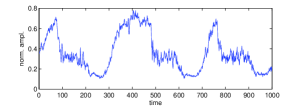
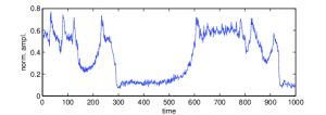
Fig.  1: Example X-ray radiation regimes $\beta$ (left) and $\kappa$ (right).

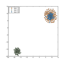
(a) NARMA by t-SNE.

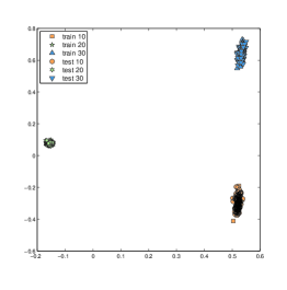
(b) NARMA by our method.

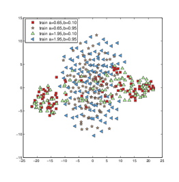
(c) Cauchy by t-SNE.

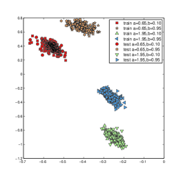
(d) Cauchy by our method.

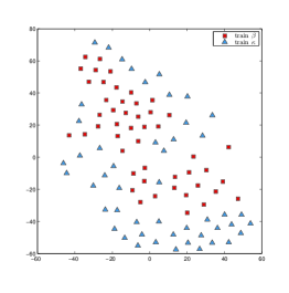
(e) X-ray radiation by t-SNE.

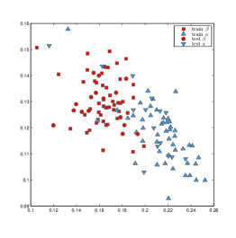
(f) X-ray radiation by our method.

Fig.  2: Colours represent classes. The proposed algorithm supports out-of-sample visualisation, hence markers $\bullet$ and $\blacktriangle$ are the projections of the training and testing data respectively. Note that in the NARMA and Cauchy plots $\bullet$ and $\blacktriangle$ heavily overlap.

We present results on two synthetic datasets and on a real astronomical dataset. In all experiments we constructed the ESN reservoir deterministically according to [7] and fixed the size of the reservoir to $N=200$. We used a washout period of $200$ observations. Regularisation parameter $\lambda$ for the ESNs was fixed to $10^{-4}$. The number of neurons in the hidden layers of the autoencoder was set to $10$. The proposed algorithm can handle out-of-sample data and hence apart from projecting training data only, we also project unseen test data. We apply no normalisation to the datasets. Moreover, we also constructed visualisations using the popular t-SNE algorithm [8] on the raw signals. We found the visualisation produced by t-SNE did not differ greatly over a range of perplexities $\{5,10,\dots,50\}$.

NARMA: We generated sequences from the following NARMA classes [7] of order $10,20,30$, of length $800$, using the following equations respectively:

$$y(t+1)\!\!\!\! = \!\!\!\!0.3y(t)+0.05y(t)\sum_{i=0}^{9}y(t-i)+1.5s(t-9)s(t)+0.1,$$

$$y(t+1)\!\!\!\! = \!\!\!\!\tanh(0.3y(t)+0.05y(t)\sum_{i=0}^{19}y(t-i)+1.5s(t-19)s(t)+0.01)+0.2,$$

$$y(t+1)\!\!\!\! = \!\!\!\!0.2y(t)+0.004s(t)\sum_{i=0}^{29}y(t-i)+1.5s(t-29)s(t)+0.201,$$

where $s(t)$ are exogenous inputs generated independently and uniformly in the interval $[0,0.5)$. These time series constitute an interesting synthetic example due to the long-term dependencies they exhibit.
Cauchy class: We sampled sequences from a stationary Gaussian process with correlation function given by $c(x_{t},x_{t+h})=(1+|h|^{a})^{-\frac{a}{b}}$ [9]. We generated $4$ classes of such time series by the permutation of parameters $a\in\{0.65,1.95\}$ and $b\in\{0.1,0.95\}$. We generated from each class $100$ time series of length $2000$.

X-ray radiation from black hole binary: We used data from [10] concerning a black hole binary system that expresses various types of temporal regimes which vary over a wide range of time scales. We extracted subsequences of length $1000$ from regimes $\beta$ and $\kappa$ that were chosen on account of their similarity (see Fig. 1).

6 Discussion and Conclusion

We show the visualisations in Fig. 2. Unlike t-SNE which operates directly on the raw data, the proposed algorithm can capture the differences between the time series in the lower dimensional space. This is because our method explicitly accounts for the sequential nature of time-series; learning is performed in the space of readout weight representations and is guided by an objective function that quantifies the reconstruction error in a principled manner. Of course, the perfectly capable t-SNE is used here as a mere candidate from the class of algorithms designed to visualise vectorial data in order to demonstrate this issue. Moreover, we demonstrate that our method, by its very nature, is capable of projecting also unseen hold-out data. Future work will focus on processing large datasets of astronomical light curves.

References

- [1] J. W. Richards, D. L. Starr, N. R. Butler, J. S. Bloom, J. M. Brewer, A. Crellin-Quick, J. Higgins, R. Kennedy, and M. Rischard. On machine-learned classification of variable stars with sparse and noisy time-series data. The Astrophysical Journal, 733(1):10, 2011.
- [2] T. Jaakkola and D. Haussler. Exploiting generative models in discriminative classifiers. In NIPS, pages 487–493. The MIT Press, 1998.
- [3] T. Jebara, R. Kondor, and A. Howard. Probability product kernels. Journal of Machine Learning Research, 5:819–844, 2004.
- [4] H. Chen, F. Tang, P. Tino, and X. Yao. Model-based kernel for efficient time series analysis. In KDD, pages 392–400, 2013.
- [5] H. Jaeger. The “echo state” approach to analysing and training recurrent neural networks. Technical report, German National Research Center for Information Technology, 2001.
- [6] M. A. Kramer. Nonlinear principal component analysis using autoassociative neural networks. AICHE Journal, 37:233–243, 1991.
- [7] A. Rodan and P. Tino. Minimum complexity echo state network. IEEE Transactions on Neural Networks, 22(1):131–144, 2011.
- [8] L. van der Maaten and G. Hinton. Visualizing data using t-SNE. Journal of Machine Learning Research, 9:2579–2605, 2008.
- [9] T. Gneiting and M. Schlather. Stochastic models that separate fractal dimension and the hurst effect. SIAM Review, 46(2):269–282, 2004.
- [10] K. P. Harikrishnan, R. Misra, and G. Ambika. Nonlinear time series analysis of the light curves from the black hole system grs1915+105. Research in Astronomy and Astrophysics, 11(1), 2011.