Competing exotic quantum phases of spin-1/2 ultra-cold lattice bosons with extended spin interactions

Abstract

Advances in pure optical trapping techniques now allow the creation of degenerate Bose gases with internal degrees of freedom. Systems such as ⁸⁷Rb, ³⁹K or ²³Na in the $F=1$ hyperfine state offer an ideal platform for studying the interplay of superfluidity and quantum magnetism. Motivated by the experimental developments, we study ground state phases of a two-component Bose gas loaded on an optical lattice. The system is described effectively by the Bose-Hubbard Hamiltonian with onsite and near neighbor spin-spin interactions. An important feature of our investigation is the inclusion of interconversion (spin flip) terms between the two species, which has been observed in optical lattice experiments. Using mean-field theory and quantum Monte Carlo simulations, we map out the phase diagram of the system. A rich variety of phases is identified, including antiferromagnetic (AF) Mott insulators, ferromagnetic and AF superfluids.

I Introduction

The question of the interplay of superfluidity and internal bosonic degrees of freedom dates back many decades. At a purely conceptual level, the most straightforward issue is whether the two internal components move in, or out of phase. A generalization of Bogoliubov’s treatment to multiple species addressed this question and demonstrated that a neutral mixture of two species of charged bosons supports plasma-type excitations with oscillating charge density and also free-particle oscillations associated with mass density oscillationsBassichis (1964). An extension of this work to finite temperatures considered dilute mixtures of (unstable) ⁶He in ⁴He Colson and Fetter (1978). Coupling between bosonic species was also shown to imply that superfluid motion of one component would result in a “drag effect” in which the second component is also set in motionNepomnyashchii (1976).

Although different theoretical and experimental motivations were presented for studying multi-component bosons, in this early work, the physical system which was probably considered in the most detail was spin polarized hydrogenHecht (1959); Etters et al. (1975); Stwalley and Nosanow (1976), where a large external magnetic field prevents recombination into molecules, and the smallness of the kinetic energy relative to the binding energy permits treatment with boson statistics. The key observationSiggia and Ruckenstein (1980) was that these bosons reside in two low-lying hyperfine states, thus allowing for possible additional symmetry breaking associated with their relative occupation. The populations of the states were measured with electron spin resonancevan Yperen et al. (1983), and the nature of excitations of the “spin” degrees of freedom was shown to range from phonon-like, to free-particle-like with energy gaps, to resembling spin wavesBerlinsky (1977). For a review, see Ref. [Greytak et al., 1984].

Lattice models were also investigated. A mean field treatmentFazekas and Entel (1983) of the hard-core limit of two component bosons focussed on the effect of “antiferromagnetic” interactions, i.e. a repulsion $V$ between the different bosonic species on near-neighbor sites of a bipartite structure. Besides promoting an insulating phase where bosonic species alternate in a regular pattern, this interaction was found also to disrupt the “symmetrical condensate” in which only a single superfluid species occurs, and allow for a superfluid phase in which both species are present. It was shown that, as a function of temperature $T$, two successive second order transitions can occur. For sufficiently large $V$, as $T$ is lowered, the bosons first form a symmetric condensate and then, at a distinct, lower temperature, the asymmetrical condensate appears. We will show here that the soft-core lattice problem exhibits certain similarities with these hard core phase diagrams.

Beginning in the late 1990’s, the properties of multicomponent boson systems became of renewed interest due to applications to ultracold quantum gases. Thanks to the all-optical trapping techniqueStamper-Kurn et al. (1998), hyperfine states of ⁸⁷Rb, ³⁹K or ²³Na in optical traps could now be used to realize interesting magnetic statesStamper-Kurn et al. (1998); Ho (1998a); Ohmi and Machida (1998). In an optical lattice, it has been observed that atoms confined on the same lattice site exhibits collisions that could change their spin statesWidera et al. (2005). Such a system can be effectively described by a multi-component Bose-Hubbard model with appropriate values of the intra- and inter-component interactions, and spin-conversion matrix elementsKrutitsky and Graham (2004); Krutitsky et al. (2005). Due to the competition between spin species, the multi-component Bose-Hubbard model is expected to host novel phasesLewenstein et al. (2012); Stamper-Kurn and Ueda (2013); Krutitsky (2015) that are absent in the one-component Bose-Hubbard modelFisher et al. (1989).

Motivated by these experimental and theoretical developments for spinor bosons in optical lattices, we will study two component (spin-$1/2$) bosons on a two-dimensional lattice. We consider a very general Hamiltonian which includes not only on-site repulsion, but also near-neighbor interactions and interconversion between the species through a spin-spin coupling. We begin with a mean field theory (MFT) treatment which reveals a rich variety of magnetic patterns (unpolarized, ferromagnetic, and antiferromagnetic) accompanying the Mott and superfluid phases. Quantum Monte Carlo (QMC) calculations then are used to explore the phase diagram more exactly. In addition to showing that many aspects of the interplay between superfluidity and magnetism suggested by MFT persist, we also show that the order of the chemical potential driven superfluid-Mott phase transition depends on which Mott lobe is being considered, and even on whether commensurate density is being approached from above or below.

High precision QMC work in two and three dimensions in the absence of interconversion has previously demonstrated the existence of different Mott and superfluid phases, distinguished by their patterns of charge and spin orderCapogrosso-Sansone et al. (2010). The possibility of mixing ‘heavy’ and ‘light’ bosonic species (‘mass imbalance’) introduced additional phenomena like ferromagnetic, phase separated states, and ‘entropy squeezing’, in which the heavy species is in a Mott phase while the light species is superfluid and can act as a heat reservoir to absorb entropyHettiarachchilage et al. (2013). The effects of interconversion on these phenomena is one of the topics of the present work.

While we will explore here the phase diagrams for quite general values of the kinetic and interaction energies, we note that the precise quantitative form of the effective (pseudo) spin interaction potential for ultracold bosonic and fermionic atoms can be computed using the “degenerate internal state approximation”Santamore and Timmermans (2011). At a basic conceptual level, the coupling is similar to a true spin interaction in which the magnetic field produced by one spin couples to the second spin, but there are important differences. One of these is that, because the hyperfine states are not “real spin”, they are not generators of rotations, and hence there is no reason to expect an isotropic (“Heisenberg-like”) form $J\,\hat{\mathbf{S}}_{1}\cdot\hat{\mathbf{S}}_{2}$. Instead, the energy can be Ising or XY in character, and indeed the precise form depends on the scattering lengths of binary atom-atom collisions in the presence of an external field.

II The spin-$1/2$ model with near-neighbor spin interactions

Here we are interested in the spin-$1/2$ Bose-Hubbard HamiltonianKrutitsky and Graham (2004); Krutitsky et al. (2005) with the spin interactions extended to near-neighbor sites

$${\hat{H}}= -t\sum_{{\langle\mathbf{i}\mathbf{j}\rangle}\sigma}\left({\hat{b}}_{\sigma\mathbf{i}}^{\dagger}{\hat{b}}_{\sigma\mathbf{j}}^{\phantom{\dagger}}+{\hat{b}}_{\sigma\mathbf{j}}^{\dagger}{\hat{b}}_{\sigma\mathbf{i}}^{\phantom{\dagger}}\right)-\mu\sum_{\mathbf{i},\sigma}{\hat{n}}_{\sigma\mathbf{i}}+\frac{U_{2}}{4}\sum_{\mathbf{i}}\hat{n}^{2}_{\mathbf{i}}$$

$$+\frac{U_{0}}{2}\sum_{\mathbf{i}}{\hat{n}}_{\mathbf{i}}({\hat{n}}_{\mathbf{i}}-1)+U_{2}\sum_{\mathbf{i}}\,\left(\hat{S}^{x}_{\mathbf{i}}\hat{S}^{x}_{\mathbf{i}}-\hat{S}^{y}_{\mathbf{i}}\hat{S}^{y}_{\mathbf{i}}-\hat{S}^{z}_{\mathbf{i}}\hat{S}^{z}_{\mathbf{i}}\right)$$

$$+V\sum_{{\langle\mathbf{i}\mathbf{j}\rangle}}\left(\hat{S}^{x}_{\mathbf{i}}\hat{S}^{x}_{\mathbf{j}}-\hat{S}^{y}_{\mathbf{i}}\hat{S}^{y}_{\mathbf{j}}-\hat{S}^{z}_{\mathbf{i}}\hat{S}^{z}_{\mathbf{j}}\right).$$ (1)

In the above equation, ${\hat{b}}_{\sigma\mathbf{i}}^{\dagger}$ (${\hat{b}}_{\sigma\mathbf{i}}^{\phantom{\dagger}}$) creates (annihilates) a pseudo-spin $\sigma=\uparrow,\downarrow$ boson on site $\mathbf{i}$ of an $L\times L$ square lattice under periodic boundary conditions. ${\hat{n}}_{\mathbf{i}}={\hat{n}}_{\uparrow\mathbf{i}}+{\hat{n}}_{\downarrow\mathbf{i}}$, and $\hat{S}^{\alpha}_{\mathbf{i}}$ ($\alpha=x,y,z$) is the spin operator defined as

$$\hat{S}^{\alpha}_{\mathbf{i}}=\frac{1}{2}\sum_{\sigma\sigma^{\prime}}\,\hat{b}^{\dagger}_{\sigma\mathbf{i}}\,\vec{\sigma}_{\sigma\sigma^{\prime}}^{\alpha}\,\hat{b}_{\sigma\mathbf{i}}^{\phantom{\dagger}},$$ (2)

where $\vec{\sigma}_{\sigma\sigma^{\prime}}^{\alpha}$ are the Pauli matrices. The parameters $t$ and $\mu$ correspond to the near-neighbor (NN) hopping amplitude and chemical potential respectively. We use $t=1$ as the unit of energy. $U_{0}$ is the contact interaction, while $U_{2}$ and $V$ are on-site and NN spin-spin interactions respectively.

Using the representation Eq. (2) and taking the NN spin-spin interaction to be along the $z$-axis only, we arrive at the following model Hamiltonian

$${\hat{H}}_{z}= -t\sum_{{\langle\mathbf{i}\mathbf{j}\rangle}\sigma}\left({\hat{b}}_{\sigma\mathbf{i}}^{\dagger}{\hat{b}}_{\sigma\mathbf{j}}^{\phantom{\dagger}}+{\hat{b}}_{\sigma\mathbf{j}}^{\dagger}{\hat{b}}_{\sigma\mathbf{i}}^{\phantom{\dagger}}\right)-\mu\sum_{\mathbf{i},\sigma}{\hat{n}}_{\sigma\mathbf{i}}$$

$$+\frac{U_{0}}{2}\sum_{\mathbf{i},\sigma}{\hat{n}}_{\sigma\mathbf{i}}({\hat{n}}_{\sigma\mathbf{i}}-1)+(U_{0}+U_{2})\sum_{\mathbf{i}}\,{\hat{n}}_{\uparrow\mathbf{i}}{\hat{n}}_{\downarrow\mathbf{i}}$$

$$+\frac{U_{2}}{2}\sum_{\mathbf{i}}\left({\hat{b}}_{\uparrow\mathbf{i}}^{\dagger}{\hat{b}}_{\uparrow\mathbf{i}}^{\dagger}{\hat{b}}_{\downarrow\mathbf{i}}^{\phantom{\dagger}}{\hat{b}}_{\downarrow\mathbf{i}}^{\phantom{\dagger}}+{\hat{b}}_{\downarrow\mathbf{i}}^{\dagger}{\hat{b}}_{\downarrow\mathbf{i}}^{\dagger}{\hat{b}}_{\uparrow\mathbf{i}}^{\phantom{\dagger}}{\hat{b}}_{\uparrow\mathbf{i}}^{\phantom{\dagger}}\right)$$

$$-V\sum_{{\langle\mathbf{i}\mathbf{j}\rangle}}{\hat{S}}^{z}_{\mathbf{i}}{\hat{S}}^{z}_{\mathbf{j}}.$$ (3)

It can be seen that the onsite spin coupling $U_{2}$ has two roles. First, it shifts the strength of the contact interaction between opposite spins $n_{\uparrow\mathbf{i}}n_{\downarrow\mathbf{i}}$. Second, $U_{2}$ is also the matrix element of the conversion process which turns two identical bosons into the opposite spin species when they meet at the same site.

Eq. (3) is the Hamiltonian that will be studied in this work. It will be solved using MFT and exact stochastic Green function (SGF) quantum Monte Carlo technique. While the SGF QMC method can treat the contact spin interactions or the NN spin-spin couplings separately, a sign problem would arise if both terms were retained due to the presence of interconversion matrix elements in both. For this technical reason, we drop the conversion matrix elements of $V$ terms in Eq. (1) and study Eq. (3). The retention of the $z$-axis term gives important insights into the effects of the NN spin-spin interactions, in the same spirit that the $t$-$J_{z}$ Hamiltonian provides initial clues into the more general rotationally invariant $t$-$J$ model.

We focus on the case where $U_{2}>0$ and $V<0$, i.e., antiferromagnetic NN spin couplings. In general, the value of $U_{0}$, $U_{2}$ and $V$ will depend on details of the system (for example, scattering length between the atoms, polarization of the laser waves forming the optical lattice, detuning from the internal atomic transition etc.Krutitsky and Graham (2004)). Here we adopt the parameter regime studied in Ref. Krutitsky and Graham, 2004 where, based on known values of ⁸⁷Rb and ²³Na scattering lengths and on laser wavelengths corresponding to the $D_{1}$ resonance, $U_{2}$ is typically an order of magnitude or more smaller than $U_{0}$. In the current work, we take the value $U_{2}/U_{0}=0.1$. For the NN coupling $V$, because interaction strength typically decreases with distance, we assume the value $|V|/U_{0}<0.1$.

When $V=0$ in Eq. (3), the system was studied extensively by MFTKrutitsky and Graham (2004); Krutitsky et al. (2005) and QMC methods in one and two dimensionsde Forges de Parny et al. (2010, 2011) . In 2D and $U_{2}>0$, the ground state of the Hamiltonian features three phases: a ferromagnetic superfluid (FMSF), an unpolarized Mott insulator (MI) at even commensurate densities, and a ferromagnetic Mott phase at odd commensurate fillings. For negative $U_{2}$, it was found that the ground state never polarizesde Forges de Parny et al. (2010, 2011).

III Mean field theory

III.1 Decoupling Mean Field theory

The mean-field scheme employed in the present work is developed in Ref. Sheshadri et al., 1993; van Oosten et al., 2001. The method is based on rewriting the Hamiltonian as a sum over local terms that can be solved exactly for a fixed number of bosons. To incorporate the hopping terms, one introduces uniform SF order parameters ${\langle{\hat{b}}_{\sigma\mathbf{i}}^{\dagger}\rangle}={\langle{\hat{b}}_{\sigma\mathbf{i}}^{\phantom{\dagger}}\rangle}=\psi_{\sigma}$. Since we are interested in equilibrium states, the order parameters $\psi_{\sigma}$ can be chosen to be real. Using this ansatz, the kinetic energy terms, which are non-diagonal in boson creation and destruction operators, are decoupled as

$${\hat{b}}_{\sigma\mathbf{i}}^{\dagger}{\hat{b}}_{\sigma\mathbf{j}}^{\phantom{\dagger}}= \,({\hat{b}}_{\sigma\mathbf{i}}^{\dagger}-{\langle{\hat{b}}_{\sigma\mathbf{i}}^{\dagger}\rangle})({\hat{b}}_{\sigma\mathbf{j}}^{\phantom{\dagger}}-{\langle{\hat{b}}_{\sigma\mathbf{j}}^{\phantom{\dagger}}\rangle})$$

$$+{\langle{\hat{b}}_{\sigma\mathbf{i}}^{\dagger}\rangle}{\hat{b}}_{\sigma\mathbf{j}}^{\phantom{\dagger}}+{\hat{b}}_{\sigma\mathbf{i}}^{\dagger}{\langle{\hat{b}}_{\sigma\mathbf{j}}^{\phantom{\dagger}}\rangle}-{\langle{\hat{b}}_{\sigma\mathbf{i}}^{\dagger}\rangle}{\langle{\hat{b}}_{\sigma\mathbf{j}}^{\phantom{\dagger}}\rangle}$$

$$\approx \,({\hat{b}}_{\sigma\mathbf{i}}^{\dagger}+{\hat{b}}_{\sigma\mathbf{j}}^{\phantom{\dagger}})\psi_{\sigma}+\psi_{\sigma}^{2},$$ (4)

where in the last line we have dropped the terms that have products of fluctuations in bosonic operators on different sites.

To treat the NN spin interactions in the same decoupling scheme, we decompose the square lattice into two disjoint sublattices $A$ and $B$ and introduce real magnetic order parameters ${\langle{\hat{S}}_{A}^{z}\rangle}$, ${\langle{\hat{S}}_{B}^{z}\rangle}$ on sublattice $A$ and $B$ respectively. Under the MF approximation, the spin-spin interaction term now becomes

$$|V|\sum_{{\langle\mathbf{i}\mathbf{j}\rangle}}{\hat{S}}_{\mathbf{i}}^{z}{\hat{S}}_{\mathbf{j}}^{z}\approx \,\,z_{c}|V|\sum_{\mathbf{i}\in A}\left(\,{\hat{S}}_{\mathbf{i}}^{z}{\langle{\hat{S}}_{B}^{z}\rangle}-\frac{1}{2}{\langle{\hat{S}}_{A}^{z}\rangle}{\langle{\hat{S}}_{B}^{z}\rangle}\,\right)$$

$$+z_{c}|V|\sum_{\mathbf{j}\in B}\left(\,{\hat{S}}_{\mathbf{j}}^{z}{\langle{\hat{S}}_{A}^{z}\rangle}-\frac{1}{2}{\langle{\hat{S}}_{A}^{z}\rangle}{\langle{\hat{S}}_{B}^{z}\rangle}\,\right).$$ (5)

As before, in this form, terms that describe products of fluctuations in ${\hat{S}}_{A}^{z}$ and ${\hat{S}}_{B}^{z}$ are ignored. $z_{c}=4$ is the coordination number of the square lattice. We have also assumed that the magnetic order parameter on each sublattice is uniform. With these approximations, the final MF Hamiltonian becomes two coupled local ones for sublattices $A$ and $B$:

$${\hat{H}}_{\ell}= -z_{c}t\sum_{\sigma}({\hat{b}}_{\sigma\ell}^{\dagger}+{\hat{b}}_{\sigma\ell})\psi_{\bar{\sigma}\ell}+z_{c}t\sum_{\sigma}\psi_{\sigma\ell}\psi_{\bar{\sigma}\ell}$$

$$+\frac{U_{0}}{2}{\hat{n}}_{\uparrow\ell}({\hat{n}}_{\uparrow\ell}-1)+\frac{U_{0}}{2}{\hat{n}}_{\downarrow\ell}({\hat{n}}_{\downarrow\ell}-1)$$

$$+\frac{U_{2}}{2}\left({\hat{b}}_{\uparrow\ell}^{\dagger}{\hat{b}}_{\uparrow\ell}^{\dagger}{\hat{b}}_{\ell\downarrow}^{\phantom{\dagger}}{\hat{b}}_{\downarrow\ell}^{\phantom{\dagger}}+h.c.\right)+(U_{0}+U_{2}){\hat{n}}_{\uparrow\ell}{\hat{n}}_{\downarrow\ell}$$

$$-\mu({\hat{n}}_{\uparrow\ell}+{\hat{n}}_{\downarrow\ell})+z_{c}|V|{\hat{S}}_{\ell}^{z}{\langle{\hat{S}}_{\bar{\ell}}^{z}\rangle}-\frac{z_{c}|V|}{2}{\langle{\hat{S}}_{\ell}^{z}\rangle}{\langle{\hat{S}}_{\bar{\ell}}^{z}\rangle},$$ (6)

where $\ell=A$, $B$ ($\bar{\ell}=B$, $A$), and $\sigma=\,\uparrow,\downarrow$ ($\bar{\sigma}=\,\downarrow,\uparrow$). The coupled Hamiltonians are solved at zero temperature by iteration. Starting with an initial guess of order parameters $\psi_{\sigma\ell}$ and ${\langle{\hat{S}}^{z}_{\ell}\rangle}$, ${\hat{H}}_{A}$ and ${\hat{H}}_{B}$ can be diagonalized numerically within the bosonic occupation number basis $\{|n_{\uparrow\ell},n_{\downarrow\ell}\rangle\}$ truncated at $n_{\sigma\ell}\leq N_{\max}$. Order parameters are then updated with respect to the new MF ground state. This procedure is repeated until $\psi_{\sigma\ell}$, ${\langle{\hat{S}}^{z}_{\ell}\rangle}$ and the ground state energy $E_{g}$ are converged. We typically choose $N_{\max}=14$ to ensure that convergence is independent of $N_{\max}$. Multiple initial configurations are also used to verify that the converged MF solution do not depend on initial conditions. We benchmark our MF program by computing the phase diagram of Eq. (6) with $V=0$. The results are in agreement with previously published datade Forges de Parny et al. (2010).

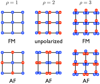
Figure 1: (Color online) Schematic diagram of ferromagnetic, antiferromagnetic, and unpolarized states at different commensurate fillings. Blue ($+$) and red ($-$) circles represent spin-up and spin-down components respectively.

Different MF phases are classified by the corresponding order parameters. For example, a superfluid is characterized by finite total superfluid density

$$\rho_{s,\ell}=\rho_{s,\uparrow\ell}+\rho_{s,\downarrow\ell}=\psi_{\uparrow\ell}^{2}+\psi_{\downarrow\ell}^{2}.$$ (7)

The Mott insulator, on the other hand, is defined by zero superfluid density $\rho_{s,\ell}=0$ and zero compressibility $\partial\rho_{\ell}/\partial\mu=0$, where

$$\rho_{\ell}=\rho_{\uparrow\ell}+\rho_{\downarrow\ell}.$$ (8)

To examine magnetic order, we compute the expectation value of ${\hat{S}}^{z}$ with respect to the converged MF solution. In a Mott phase, this is

$$S^{z}_{\ell} =\frac{1}{2}{\langle{\hat{n}}_{\uparrow\ell}-{\hat{n}}_{\downarrow\ell}\rangle},$$ (9)

where ${\hat{n}}_{\sigma\ell}$ is the density operator. In principle one can use Eq. (9) in the SF phase, and the conclusion should remain the same. Here we follow the convention in Ref. Ho, 1998b; Krutitsky and Graham, 2004 and compute the magnetization in the SF phase defined as

$$S^{z}_{s,\ell}=\frac{1}{2}\frac{\psi_{\uparrow\ell}^{2}-\psi_{\downarrow\ell}^{2}}{\rho_{s,\ell}},$$ (10)

which merely measures the SF population difference between the two spin components.

Figure 1 summarizes schematically the possible magnetic structures at three commensurate fillings. For example, the state (SF or MI) is ferromagnetic (FM) if one of the spin components dominates the population throughout the lattice. An unpolarized state has both spin components equally occupied on every lattice site. An antiferromagnetic (AF) state is realized when sublattices $A$ and $B$ are dominated by different spin species.

III.2 Mean Field Results

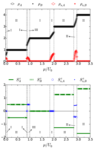
Figure 2: (Color online) Features of the MF ground state as a function of chemical potential $\mu/U_{0}$ at $t/U_{0}=0.02$, $U_{2}/U_{0}=0.1$ and $|V|/U_{0}=0.02$. Total particle and total superfluid densities on $\ell=A$ and $B$ sublattices are plotted in the top panel. Magnetic order parameters $S^{z}_{\ell}$ and $S^{z}_{s,\ell}$ are shown in the bottom panel. In both figures, the vertical dashed lines divide the phases into various zones based on their magnetic structures labeled by the roman numerals: I – unpolarized, II – AF, and III – FM. Note that the changes in sign of $S^{z}_{A}$ ($S^{z}_{B}$) in the first Mott plateau are a trivial reflection of the degeneracy of the two MF solutions.

Properties of the MF ground state are shown in Fig. 2 for $t/U_{0}=0.02$, $U_{2}/U_{0}=0.1$, and $|V|/U_{0}=0.02$. Total particle and SF densities are plotted in the upper figure as functions of $\mu/U_{0}$. The density develops three well defined plateaux at $\rho=1$, 2, and 3. These plateaux correspond to MIs because the compressibility $\partial\rho/\partial\mu=0$ and the SF density also vanishes. The SF phase resides in between the Mott insulators. It can be seen that $\rho_{\ell}$ and $\rho_{s,\ell}$ change discontinuously when one enters and leaves the first Mott plateau. This is the signature of a first order phase transition. Likewise, the transition is also first order as one enters the $\rho=3$ MI from below. On the other hand, $\rho_{\ell}$ and $\rho_{s,\ell}$ change continuously on both sides of the second Mott plateau, indicating that the MI-SF transition is second order.

The lower panel of Fig. 2 summarizes MF magnetic structures for $t/U_{0}=0.02$, $U_{2}/U_{0}=0.1$, and $|V|/U_{0}=0.02$. Within the $\rho=1$, 3, and 4 plateaux, the magnetic order parameter on sublattices $A$ and $B$ are equal but have opposite signs $S^{z}_{A}=-S^{z}_{B}$. This shows that these MIs are antiferromagnetic. In contrast, the second Mott insulating region is non-magnetic. In the SF region, magnetic properties are plotted by blue symbols (dots and empty circles). The SF between the $\rho=1$ and $\rho=2$ Mott regions has two different magnetic natures: unpolarized and fully polarized. The transition between them is first order. This is also indicated in the upper panel by a discontinuity in $\rho_{s,\ell}$. Most interestingly, the SF above the $\rho=3$ Mott region shows antiferromagnetic structure.

By carrying out the self-consistent MF calculation at different $t/U_{0}$ (or $\mu/U_{0}$) values, the $\mu$-$t$ phase diagram can be constructed. Results for $|V|/U_{0}=0.02$ and 0.08 are plotted in Fig. 3. Here red (solid) and blue (dashed) curves represent first and second order phase transitions respectively. Comparing with the $V=0$ phase diagramde Forges de Parny et al. (2010), there are several notable changes due to the presence of NN spin-spin couplings.

The magnetic structure of the first and third Mott lobes changes from being ferromagnetic to antiferromagnetic. At $\rho=1$ or 3, one of the spin components dominates the population. As a result, the MF ground state energy can be lowered by forming an AF pattern. At $\rho=2$, on the other hand, the onsite coupling term can be effectively avoided by equally populating both spin species on every site if $|V|/U_{0}=0.02$ is small. By raising $|V|/U_{0}$ to 0.08, the second lobe also becomes antiferromagnetic. This is because the energy gained by forming an AF state compensates the energy cost of onsite coupling terms at large $|V|/U_{0}$ values.

When $V=0$, the MI-SF phase transition is continuous except for the tip of the second Mott lobe. The transition is known to be first order for $0<U_{2}/U_{0}\lesssim 0.25$.de Forges de Parny et al. (2010) Here we find that the transition becomes first order due to the change of magnetic property in the $\rho=1$ and 3 Mott lobes. Note that above the third lobe, the antiferromagnetic Mott insulator to antiferromagnetic superfluid (AFSF) transition remains continuous. At $|V|/U_{0}=0.08$, the bottom half of the phase boundary enclosing the Mott insulators is first order; while the upper half becomes continuous.

Regarding the magnetic structure of the SF phase, it was found that the SF is always polarized if $V=0$de Forges de Parny et al. (2010). With the presence of NN spin-spin couplings, an unpolarized SF emerges near the Mott lobes, particularly at small $t/U_{0}$ values. An exception to this observation is found at $\rho>3$ where an AFSF phase occupies the region between the third and fourth MIs. At $|V|/U_{0}=0.08$, the AFSF region expands dramatically to large hopping regions, and to chemical potential values as low as $\mu/U_{0}\sim 0.6$. This AFSF is a supersolid phase since it exhibits simultaneous diagonal and off-diagonal long range order.

Recall that in the original Bose-Hubbard modelFisher et al. (1989) or in the case $V=0$ in Eq. (6)de Forges de Parny et al. (2010, 2011), the SF phase extends all the way to $t/U_{0}=0$. Fig. 3 shows that this is no longer the case when $V$ is turned on. The system undergoes a series of first-order transition between MIs at small $t/U_{0}$.

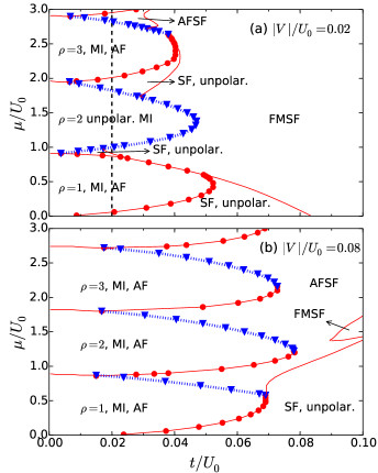
Figure 3: (Color online) MF phase diagrams obtained by solving the coupled Hamiltonian Eq. (6) for $U_{2}/U_{0}=0.1$. The NN spin interaction strength $|V|/U_{0}$ is (a) 0.02 and (b) 0.08. First order and continuous phase transitions are represented by red (solid) and blue (dashed) curves respectively. “AF”, “FM”, and “unpolar” indicate magnetic structures. At $|V|/U_{0}=0.02$, an AFSF phase emerges between the $\rho=3$ and $4$ Mott lobes. With increasing $|V|/U_{0}$, the AFSF region expands significantly. Moreover, the $\rho=2$ lobe changes its nature from being non-magnetic at $|V|/U_{0}=0.02$ to antiferromagnetic at $|V|/U_{0}=0.08$. In panel (a), the vertical dashed line indicates the location of $t/U_{0}$ where Fig. 2 is plotted.

IV Exact Quantum Monte Carlo Study

In this section, we solve the model Eq. (3) exactly on finite lattices by using Stochastic Green Function (SGF) QMCRousseau (2008). The SGF method is a finite-temperature continuous time QMC technique that can be formulated in either the canonical or grand canonical ensembles. The SGF algorithm can solve a large class of lattice Hamiltonians that can be written as ${\hat{H}}={\hat{V}}-{\hat{T}}$, where ${\hat{V}}$ is diagonal in the Fock basis (subject to the model type) and ${\hat{T}}$ has only positive elementsRousseau (2008). The technique has also been applied to the $V=0$ case of Eq. (3) in one and two dimensionsde Forges de Parny et al. (2010, 2011).

In our simulations, the temperature is set at $\beta t=2L$ for a lattice with linear dimension $L$. The chosen temperature is typically low enough to ensure that the results are converged to the ground state limit. In some cases, we select $\beta t=4L$ to reach convergence. We benchmarked the SGF algorithm by comparing with exact diagonalization data for a small cluster. The SGF and exact results are in agreement within statistical errors.

IV.1 Phase diagram

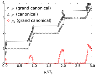
Figure 4: (Color online) Particle density $\rho$ (square and triangle) and SF density $\rho_{s}$ (diamond) versus chemical potential computed using the SGF QMC method for $t/U_{0}=0.02$. For comparison, we have implemented canonical and grand canonical ensembles in the simulations. Both data sets are acquired on a $L=6$ lattice at temperature $\beta=12$. Conversion term and NN spin interactions are $U_{2}/U_{0}=0.1$ and $|V|/U_{0}=0.02$ respectively. The canonical ensemble results are shifted upward by 0.5 for clarity. The signature of first order transition (discontinuous jump in $\rho$ and $\rho_{s}$ in the grand canonical ensemble curve, and negative compressibility $\partial\rho/\partial\mu<0$ in the canonical ensemble data) can be seen at both ends of the first Mott lobe and the bottom boundary of the third lobe.

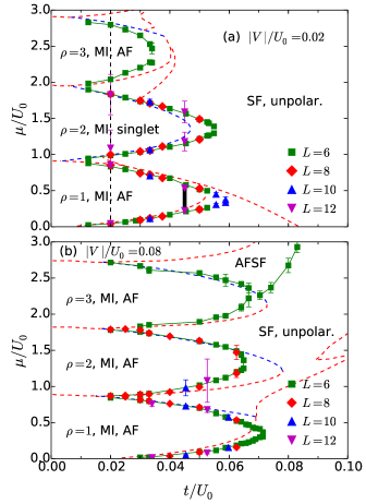
Figure 5: (Color online) Exact phase diagram of the Hamiltonian Eq. (3) obtained using the SGF QMC technique on $L\times L$ lattices at temperature $\beta=2L$. The onsite spin coupling is fixed at $U_{2}/U_{0}=0.1$. The NN spin-spin interaction $|V|/U_{0}$ is set at (a) 0.02 and (b) 0.08. Statistical uncertainties are typically smaller than the symbol size. The vertical dashed line is the location where Fig. 4 is plotted. Mean-field phase boundaries are also presented (dashed curves) for comparison. In (a), the vertical heavy line in the $\rho=1$ Mott lobe near the tip is the location of magnetic transition (c.f. Fig. 7). In (b), AFSF is predicted to exist in the region above the $\rho=3$ MI.

To construct the exact phase diagram, we compute the total particle density $\rho$ and SF density $\rho_{s}$ as functions of chemical potential. In canonical ensemble SGF simulations, the total particle number $N$ is fixed, and we derive the chemical potential via

$$\mu(N)=E(N+1)-E(N),$$ (11)

where $E(N)$ is the total energy of $N$ bosons on an $L\times L$ lattice. To access the SF density, we use the formula proposed by Pollock and CeperleyPollock and Ceperley (1987), which relates $\rho_{s}$ to the winding number $W$. However, due to the conversion term in the Hamiltonian Eq. (3), the numbers of spin $\uparrow$ and $\downarrow$ bosons are not conserved individually. As a consequence, the relevant winding number should take into account both spin componentsEckholt and Roscilde (2010) and $\rho_{s}$ is given by the following formula

$$\rho_{s}=\frac{{\langle(W_{\uparrow}+W_{\downarrow})^{2}\rangle}}{2dt\beta L^{d-2}},$$ (12)

where $d=2$ is the dimensionality, $t$ is the hopping amplitude, and $W_{\uparrow}$ and $W_{\downarrow}$ are the winding numbers of spin $\uparrow$ and $\downarrow$ bosons respectively.

Figure 4 shows QMC results for $\rho$ and $\rho_{s}$ versus $\mu/U_{0}$ on the $L=6$ lattice with $t/U_{0}=0.02$, $U_{2}/U_{0}=0.1$, and $|V|/U_{0}=0.02$. We compare total densities $\rho(\mu)$ measured using both grand canonical (square) and canonical (triangle) ensembles. Three plateaux can be observed at commensurate fillings. Since the compressibility $\partial\rho/\partial\mu$ and superfluid density $\rho_{s}$ vanish in the plateaux, these regions represent Mott insulators. In between the Mott insulators there is a SF with $\rho_{s}\neq 0$. The agreement of the data for different ensembles acts both as a check of our codes and also as an assessment of finite size effects, since equivalence is expected only for sufficiently large lattices.

In Fig. 4, the grand canonical ensemble particle density has a discontinuous jump when one enters or leaves the first Mott region. These jumps show that the MI-SF transition is first order. This is confirmed by the canonical ensemble data which clearly indicates negative compressibility $\partial\rho/\partial\mu<0$ in the same region. At the same time, the SF density shows a discontinuous jump. Likewise, the MI-SF transition near $\mu/U_{0}\sim 2.1$ is first order. The transition at $\rho=2$ is second order as both quantities $\rho$ and $\rho_{s}$ change continuously (within the resolution of our $\mu/U_{0}$ grid) as a function of the chemical potential. MF predictions at $t/U_{0}=0.02$ (cf. Fig. 2) are consistent with these exact QMC results.

The QMC phase diagram is shown in Fig. 5 for (a) $|V|/U_{0}=0.02$ and (b) $|V|/U_{0}=0.08$. The onsite spin coupling strength is $U_{2}/U_{0}=0.1$ in both cases. The corresponding MF phase boundaries (dashed curves) are also plotted for comparison. The QMC data are shown for $\mu/U_{0}\lesssim 2.75$ as it becomes increasingly difficult to reduce statistical errors for simulation at large chemical potential values. System sizes $L=6$, 8, 10, and 12 are used, with little variation evident on the QMC phase boundaries. Overall, the QMC and MF phase boundaries are in good agreement, especially at small $t/U_{0}$ where the MF assumption works well. The deviation between the two approaches increases as one moves toward the tips of the Mott lobes where quantum fluctuations are large. Interestingly, at $/U_{0}=0.02$ and near $t/U_{0}\sim 0.045$, our QMC data reveal a magnetic phase transition inside the first MI. The transition is indicated by a thick black line in Fig. 5 and will be discussed in the next subsection. At $|V|/U_{0}=0.08$, the QMC Mott insulating regions expand, which is consistent qualitatively with MF results. At small $t/U_{0}$ values, our QMC data also suggest the existence of a direct first-order MI-MI transition at both $|V|/U_{0}=0.02$ and 0.08, confirming the MF predictions.

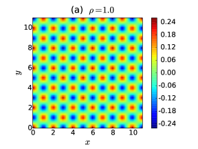
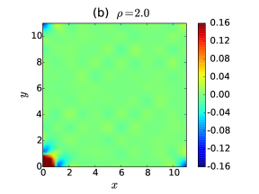
Figure 6: (Color online) Spin-spin correlation function $C^{zz}(\mathbf{r})$ for the (a) $\rho=1$ and (b) $\rho=2$ Mott insulators. The data are measured on an $L=12$ lattice for $t/U_{0}=0.02$, $U_{2}/U_{0}=0.1$, and $|V|/U_{0}=0.02$. The data show that the first lobe has AF order while the second lobe is non-magnetic.

IV.2 Magnetic properties of the Mott lobes

Figure 7: (Color online) Normalized antiferromagnetic spin structure factor $S^{zz}(\pi,\pi)/L^{2}$ and SF density $\rho_{s}$ as functions of hopping amplitude $t/U_{0}$. Here $U_{2}/U_{0}=0.1$ and $|V|/U_{0}=0.02$. In panel (a), the data are plotted near the tip of the $\rho=1$ Mott lobe of the phase diagram Fig. 5. AF order is destroyed at $t/U_{0}\sim 0.045$, before the system becomes a SF near $t/U_{0}\sim 0.06$. The shaded region denotes the non-magnetic Mott insulator. In panel (b), the same observables are plotted at $\rho=3$. Here the insulator-to-SF and magnetic transitions take place at the same critical values $t/U_{0}\sim 0.39$ and is first order.

To study magnetic properties of the model in QMC simulations, we measure the real-space spin-spin correlation function along the $z$-axis

$$C_{s}(\mathbf{r})=\frac{1}{L^{2}}\sum_{\mathbf{r}^{\prime}}{\langle{\hat{S}}^{z}_{\mathbf{r}+\mathbf{r}^{\prime}}{\hat{S}}^{z}_{\mathbf{r}^{\prime}}\rangle}.$$ (13)

Figure 6 shows the results obtained for the $L=12$ lattice at $\rho=1$ (upper panel) and $\rho=2$ (lower panel) with $U_{2}/U_{0}=0.1$, $|V|/U_{0}=0.02$, and $t/U_{0}=0.02$, i.e. inside the MI phases. The staggered correlation pattern displayed in Fig. 6 (a) shows that the first Mott lobe is antiferromagnetic. Similar results are also obtained for the third lobe. As indicated by Fig. 6 (b), the second Mott lobe at $|V|/U_{0}=0.02$ is non-magnetic since only short-ranged correlation exists.

In order to confirm that the $\rho=1$ and 3 MIs have long-range magnetic order, we have also studied the scaling of the spin structure factor at $(\pi,\pi)$

$$S^{zz}(\pi,\pi)=\sum_{\mathbf{r}}(-1)^{\mathbf{r}}C_{s}(\mathbf{r}).$$ (14)

If the state has a long-range AF order, then $S^{zz}(\pi,\pi)$ should scale as $L^{2}$Huse (1988). The results for the first Mott lobe at $U_{2}/U_{0}=0.1$ and $|V|/U_{0}=0.02$ are plotted in Fig. 7 (a) as a function of $t/U_{0}$. In this figure, the filled symbols represent $S^{zz}(\pi,\pi)/L^{2}$ computed for $L=6$, 8, 10, and 12. The data confirm that the first Mott lobe has long-range AF order. By carrying out similar scaling studies, we have verified that the third lobe at $U_{2}/U_{0}=0.1$, $|V|/U_{0}=0.02$ (cf. Fig. 7 (b)), and the $\rho=1$, 2, and 3 MI phases at $U_{2}/U_{0}=0.1$, $|V|/U_{0}=0.08$ also have long-range AF order. These findings confirm the MF predictions regarding the magnetic structure of Mott insulators at commensurate fillings in the parameter ranges studied.

In addition to the AF order parameter $S^{zz}(\pi,\pi)$, we also show in Fig. 7 the total SF density as a function of $t/U_{0}$ for $|V|/U_{0}=0.02$. It can be seen that at $\rho=1$, the SF density $\rho_{s}$ rises and becomes size-independent (indicating a true SF phase) at $t/U_{0}\sim 0.06$, a value that is consistent with the one found in Fig. 5 (a). Therefore, as one scans through $t/U_{0}$, the $\rho=1$ Mott insulator undergoes a first order (indicated by the discontinuous jump in $S^{zz}(\pi,\pi)/L^{2}$) magnetic phase transition at $t/U_{0}\sim 0.045$ before it becomes a SF. This magnetic phase transition is not captured by the MF theory.

Figure 7(b) shows a similar analysis near the tip of the third MI phase at $|V|/U_{0}=0.02$. It is found that the MI-SF transition is first order and takes place at $t/U_{0}\sim 0.037$. However, no intermediate phase exists.

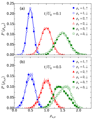
Figure 8: (Color online) Histogram of the SF density $P(\rho_{s,\sigma})$ for $\sigma=\uparrow$ and $\downarrow$ bosons at three different commensurate fillings $\rho_{s}=\rho_{s,\uparrow}+\rho_{s,\downarrow}$. The system is a $L=6$ lattice with $U_{2}/U_{0}=0.1$, $|V|/U_{0}=0.02$, and $\beta=12$. In case (a) where $t/U_{0}=0.1$, the probability $P(\rho_{s,\sigma})$ centers at $\rho_{s}/2$, indicating that both spin components are equally populated in the SF state. In case (b) $t/U_{0}=0.5$, there is an asymmetry between $P(\rho_{s,\uparrow})$ and $P(\rho_{s,\downarrow})$ at $\rho_{s}=3$. This implies that the SF state has a finite polarization.

IV.3 Magnetic properties of the SF phase

Next we turn our attention to magnetic properties of the SF phase. MFT predicts three different types of SF: a FMSF, an AFSF, and an unpolarized SF. At $|V|/U_{0}=0.02$, the FMSF dominates the phase diagram. At a stronger NN spin coupling $|V|/U_{0}=0.08$, the AFSF becomes the major component(cf. Fig. 3).

To verify these MF predictions, we first compute the SF density histogram $P(\rho_{s,\sigma})$ for spin $\sigma=\uparrow$ and $\downarrow$ bosons. As shown in previous resultsde Forges de Parny et al. (2010, 2011), $P(\rho_{s,\sigma})$ for $\sigma=\uparrow$ and $\downarrow$ are identical if both spin species are equally populated. On the other hand, $P(\rho_{s,\uparrow})$ and $P(\rho_{s,\downarrow})$ would peak at different values of $\rho_{s,\sigma}$ if the superfluid develops polarization.

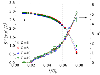
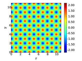
Figure 9: (Color online) Upper panel : Antiferromagnetic spin structure factor $S^{zz}(\pi,\pi)$ and SF density $\rho_{s}$ versus $t/U_{0}$ measured at $\rho=3.5$. The onsite and NN spin interactions are $U_{2}/U_{0}=0.1$ and $|V|/U_{0}=0.08$ respectively. The system is a SF for $t/U_{0}\gtrsim 0.02$. Within the SF phase, $S^{zz}(\pi,\pi)$ scales as $L^{2}$. These results suggest that the SF has long-range AF order. Lower panel: Spin-spin correlation function $C_{s}(\mathbf{r})$ computed on the $L=12$ lattice at the $t/U_{0}=0.0588$, indicated by the dashed vertical line in the upper panel.

At $U_{2}/U_{0}=0.1$ and $|V|/U_{0}=0.02$, examples of the histogram are plotted in Fig. 8(a) for the $L=6$ lattice at three commensurate densities $\rho_{s}=\rho_{s,\uparrow}+\rho_{s,\downarrow}=1$, 2, 3 at $t/U_{0}=0.1$, i.e. deep inside the SF phase. The figure shows that $P(\rho_{s,\sigma})$ are identical for both spin components at a given density and peaks at $\rho_{s}/2$, indicating no spin polarization. We find no FMSF in the parameter range shown in the $|V|/U_{0}=0.02$ QMC phase diagram (top panel of Fig. 5).

In order to search for the FMSF further, we carry out the simulation at much higher $t/U_{0}$ values. One representative result of $P(\rho_{s,\sigma})$ at $t/U_{0}=0.5$ is depicted in Fig. 8(b) for the $L=6$ lattice with $U_{2}/U_{0}=0.1$ and $|V|/U_{0}=0.02$. The figure shows that at $\rho_{s}=1$, 2, and 3, the histogram peaks at different locations for different spin species. These results suggest the existence of a spin polarized SF phase, albeit at a much higher hopping range than the MF prediction. A similar conclusion is reached at $|V|/U_{0}=0.08$ for the FMSF phase.

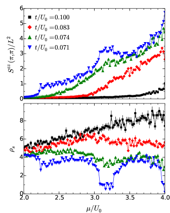
Figure 10: (Color online) Normalized spin structure factor at $(\pi,\pi)$ (top panel) and superfluid density (bottom panel) versus chemical potential $\mu/U_{0}$ computed on the $L=6$ lattice with $U_{2}/U_{0}=0.1$, $|V|/U_{0}=0.08$. In the top panel, there is a sudden increase in $S^{zz}(\pi,\pi)$ near $\mu/U_{0}\sim 2.2$, 3.1, and 3.9 for $t/U_{0}=0.071$. At roughly the same $\mu/U_{0}$ values and the same $t/U_{0}$, a reduction in $\rho_{s}$ can been observed.

To probe the AFSF phase, we compute the spin correlation function Eq. (13) in the superfluid phase. At $|V|/U_{0}=0.02$, results only indicate short-range AF correlations, and the corresponding scaling study of AF spin structure factor does not support any long-range AF order in the superfluid.

We carry out the same analysis for $|V|/U_{0}=0.08$, and the results at $\rho=3.5$ are summarized in Fig. 9. The upper panel of the figure shows $S^{zz}(\pi,\pi)/L^{2}$ as well as total SF density $\rho_{s}$ in a range of $t/U_{0}$ values. The superfluid density data indicate the onset of superfluidity is at $t/U_{0}\sim 0.02$. In the SF phase, the AF spin structure factor is finite and scales as $L^{2}$ before it drops to zero at $t/U_{0}\sim 0.08$. These data combined therefore confirm the existence of an AFSF phase at $|V|/U_{0}=0.08$. This phase can be considered a supersolid phase since it exhibits similtaneous digaonal and off-diagonal long range order. In the lower panel of Fig. 9, we show a real-space spin correlation function result acquired on an $L=12$ lattice at $\rho=3.5$, $U_{2}/U_{0}=0.1$, $|V|/U_{0}=0.08$, and $t/U_{0}=0.0588$ (indicated by the vertical dashed line in the upper panel of Fig. 9). The staggered correlation function pattern demonstrates the long range antiferromagnetic structure of the SF phase. This long range AF order in the SF phase appeared as the NN repulsion was increased from $|V|/U_{0}=0.02$ to $|V|/U_{0}=0.08$. We have not, however, determined the value of $|V|/U_{0}$ at which the AFSF first appears.

Figure 9 also indicates that at some values of $t/U_{0}$, the AF order vanishes and the SF becomes a normal superfluid. To estimate the exact phase boundary of this AFSF to normal SF transition, we have conducted a series of grand canonical and canonical SGF simulations and extracted $S^{zz}(\pi,\pi)$ as a function of $\mu/U_{0}$ for several $t/U_{0}$ values. A set of data is presented in Fig. 10 for the $L=6$ lattice with $U_{2}/U_{0}=0.1$, $|V|/U_{0}=0.08$, and $2\leq\mu/U_{0}\leq 4$. It can be seen from the figure that the transition from a normal SF to AFSF takes place at a chemical potential value much higher than the MF result, and the critical $\mu/U_{0}$ increases with $t/U_{0}$. We have done similar calculations for other system sizes. The estimated AFSF phase boundary is shown in Fig. 5 (b).

Finally, we would like to remark that as one scans the chemical potential in the range $2\leq\mu/U_{0}\leq 4$ at $t/U_{0}=0.071$, a reduction in the SF density at $\mu/U_{0}\sim 2.2,3.1$ and $3.9$ can be observed in Fig. 10. Correspondingly, $S^{zz}(\pi,\pi)$ rises rapidly near these $\mu/U_{0}$ values. Because $t/U_{0}=0.071$ is just outside the tip of the third Mott lobe, the reduction in $\rho_{s}$ at $\mu/U_{0}=2.2$ is caused by the proximity effect of the third MI phase. The reduction in $\rho_{s}$ at $\mu/U_{0}\sim 3.1$ indicates indirectly the location of the tip of the fourth AF Mott lobe (and potentially the fifth at $\mu/U_{0}\sim 3.9$).

V Conclusion

In this work, we have used the site-decoupling MF theory and the exact SGF QMC algorithm to study the ground state phase diagram of the Bose-Hubbard model with onsite and NN spin-spin couplings Eq. (3). The SGF approach allows us to treat terms which interconvert the two bosonic species. Previous studyde Forges de Parny et al. (2011) have shown that the Hamiltonian at $V=0$ and positive $U_{2}$ has three phases: a ferromagnetic Mott insulator at $\rho=1$ (and all odd Mott lobes), an unpolarized Mott phase for $\rho=2$ (and all even commensurate densities), and a ferromagnetic superfluid.

In the presence of NN interactions $|V|\sum_{{\langle\mathbf{i}\mathbf{j}\rangle}}\hat{S}^{z}_{\mathbf{i}}\hat{S}^{z}_{\mathbf{j}}$, the magnetic structures found at $V=0$ are profoundly modified. In particular, at $|V|/U_{0}=0.02$, the Mott lobes at $\rho=1$, 3 become antiferromagnetic. The Mott phase at $\rho=2$ is a spin-singlet state. The superfluid phase becomes unpolarized for $t/U_{0}\lesssim 0.5$. By increasing the strength of NN spin coupling to $|V|/U_{0}=0.08$, the second Mott lobe also becomes antiferromagnetic, and, most interestingly, an AFSF (a supersolid phase) emerges at high fillings.

At the $|V|/U_{0}$ values studied, the MF and exact QMC results are in good agreement, particularly at small $t/U_{0}$ values (deep inside the Mott phase) where quantum fluctuations are small. Moreover, the site-decoupling MFT is able to capture correctly the magnetic structure of the Mott insulators and predict the existence of AFSF. The order of MI-SF phase transition is also verified by the exact results.

Just as initial qualitative studies of the single species boson-Hubbard model were followed by quantitative comparisons with experiment Jimenez Garcia et al. (2010); Mahmud et al. (2011), a natural next step here will be to do similar modeling of multi-component bosonic optical lattice experiments. However, the complication introduced by the effect of a trap, which in the single species case manifests itself as the coexistence of superfluid, Mott insulator, and normal phases as $\rho$, $U/t$ and $T/t$ vary across the cloud, will be even more challenging, since the possibility of magnetic order introduces additional phases which might coexist in the presence of a confining potential.