The Coronal Temperatures of Low-Mass Main-Sequence Stars

Abstract

Aims. We study the X-ray emission of low-mass main-sequence stars to derive a reliable general scaling law between coronal temperature and the level of X-ray activity.

Methods. We collect ROSAT measurements of hardness ratios and X-ray luminosities for a large sample of stars to derive which stellar X-ray emission parameter is most closely correlated with coronal temperature. We calculate average coronal temperatures for a sample of 24 low-mass main-sequence stars with measured emission measure distributions (EMDs) collected from the literature. These EMDs are based on high-resolution X-ray spectra measured by XMM-Newton and Chandra.

Results. We confirm that there is one universal scaling relation between coronal average temperature and surface X-ray flux, $F_{\text{X}}$, that applies to all low-mass main-sequence stars. We find that coronal temperature is related to $F_{\text{X}}$ by $\bar{T}_{\text{cor}}=0.11F_{\text{X}}^{0.26}$, where $\bar{T}_{\text{cor}}$ is in MK and $F_{\text{X}}$ is in erg s^-1 cm^-2.

1 Introduction

Figure 1: Plots showing how different measures of X-ray emission scale with hardness ratio for stars of different masses. The hardness ratios and levels of X-ray emission were measured by ROSAT and collected using the NEXXUS database (Schmitt & Liefke 2004). The blue and red points represent stars with masses below and above 0.65 M_⊙ respectively. The three quantities of interest are X-ray luminosity (left panel), X-ray surface flux (middle panel), and X-ray luminosity divided by the bolometric luminosity (right panel). In order to calculate $F_{\text{X}}$ and $R_{\text{X}}$ we estimate the surface areas and the bolometric luminosities by assuming $R_{\star}\propto M_{\star}^{0.8}$ and $L_{\text{bol}}\propto M_{\star}^{3.9}$.

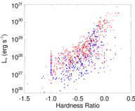
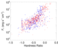
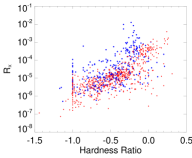
The X-ray emission properties of low-mass main-sequence stars are strongly dependent on stellar mass and rotation (Vilhu 1984; Pizzolato et al. 2003). Although the basic physical mechanisms responsible for heating coronae to X-ray emitting temperatures are not well understood, it is known empirically that coronal temperatures correlate well with levels of X-ray emission (Vaiana 1983; Schrijver et al. 1984; Schmitt et al. 1990; Schmitt et al. 1995; Güdel et al. 1997; Schmitt 1997; Telleschi et al. 2005; Telleschi et al. 2007). For example, Telleschi et al. (2005) analysed high-resolution XMM-Newton spectra of six solar analogues with different levels of magnetic activity and showed that $L_{\text{X}}\propto\bar{T}_{\text{cor}}^{4.05\pm 0.25}$, where $\bar{T}_{\text{cor}}$ is the emission measure weighted average coronal temperature (given by Eqn. 1).

An important question is which measure of X-ray emission correlates best with coronal temperature for stars with a range of surface areas and spectral types; the three obvious candidates are X-ray luminosity, $L_{\text{X}}$, X-ray luminosity normalised by the bolometric luminosity, $R_{\text{X}}=L_{\text{X}}/L_{\text{bol}}$, and X-ray surface flux, $F_{\text{X}}=L_{\text{X}}/(4\pi R_{\star}^{2})$. Schmitt (1997) compared ROSAT hardness ratio measurements for a sample of main-sequence F and G stars with similar measurements for a sample of main-sequence K and M stars and concluded that all low-mass main-sequence stars have the same relation between surface flux and spectral hardness. Similarly, Preibisch (1997) analysed ROSAT spectra for a sample of stars and argued that $F_{\text{X}}$ is a better measure than $L_{\text{X}}$, though they did not consider the parameter $R_{\text{X}}$.

The answer to which of these parameters is best correlated with coronal temperature could contribute to our understanding of the magnetic processes responsible for heating coronal plasma to X-ray emitting temperatures and to our understanding of the coronal properties of saturated stars. For example, if $R_{\text{X}}$ is the relevant parameter, then this would indicate that temperature scales somehow with how far a star is below the saturation threshold in rotation, given that saturation happens at a single mass-independent value of $R_{\text{X}}$. It would further imply that all saturated stars have similar coronal temperatures. On the other hand, if either $L_{\text{X}}$ or $F_{\text{X}}$ are the relevant parameters, then it would indicate that among stars that lie above the saturation threshold, lower mass stars have cooler coronae than their higher mass counterparts. The answer can also important for our understanding of stellar radiation in X-rays since stars with hotter corona will emit more photons at higher energies for a given total X-ray flux. This could be important for our understanding of the influences of stars on the upper atmospheres of planets, given that the influence that high-energy radiation has on a planet is highly wavelength dependent (Tian et al. 2005; Cecchi-Pestellini et al. 2009; Chadney et al. 2015).

In this paper, we analyse coronal temperatures for a large sample of stars with different masses to show that $F_{\text{X}}$ is indeed the best indicator of coronal temperature and to derive a general scaling law that can be used to predict $\bar{T}_{\text{cor}}$ for all low-mass main-sequence stars. In Section 2, we analyse ROSAT measurements of hardness ratio for a sample of nearby X-ray emitting stars. In Section 3, we calculate $\bar{T}_{\text{cor}}$ for a sample of stars based on high-resolution XMM-Newton and Chandra spectra and show how it correlated with $F_{\text{X}}$.

Name	$R_{\star}$	$F_{\text{X}}$	$\bar{T}_{\text{cor}}$	Reference
	(R⊙)	(erg s-1 cm-2)	(MK)
Solar Min	1.00	$4.44\times 10^{3}$	0.97	1
$\alpha$ Cen A	1.24	$2.46\times 10^{4}$	1.49	2
$\alpha$ Cen B	0.84	$5.60\times 10^{4}$	1.76	2
Solar Max	1.00	$7.73\times 10^{4}$	2.57	1
SCR 1845	0.10	$2.30\times 10^{5}$	2.30	3
$\beta$ Com	1.1013	$2.47\times 10^{5}$	3.89	4
Prox Cen	0.1414	$3.36\times 10^{5}$	2.70	5
$\xi$ Boo B	0.61	$4.13\times 10^{5}$	2.23	6
70 Oph A	0.85	$4.24\times 10^{5}$	3.39	7
36 Oph B	0.59	$4.31\times 10^{5}$	2.71	7
36 Oph A	0.69	$4.35\times 10^{5}$	2.82	7
70 Oph B	0.66	$4.65\times 10^{5}$	3.23	7
$\epsilon$ Eri	0.78	$5.65\times 10^{5}$	3.48	7
$\pi^{3}$ Ori	1.3215	$8.61\times 10^{5}$	4.31	8
$\chi^{1}$ Ori	1.0213	$1.41\times 10^{6}$	4.37	4
$\kappa^{1}$ Ceti	0.9313	$1.70\times 10^{6}$	4.57	4
$\xi$ Boo A	0.83	$1.73\times 10^{6}$	4.37	6
$\pi^{1}$ UMa	0.9613	$2.05\times 10^{6}$	4.47	4
YZ CMi	0.36	$2.73\times 10^{6}$	5.79	9
AD Leo	0.3716	$7.04\times 10^{6}$	6.39	10
EV Lac	0.3617	$7.44\times 10^{6}$	6.78	10
AU Mic	0.8418	$1.28\times 10^{7}$	7.09	11
AB Dor	1.1019	$1.39\times 10^{7}$	9.32	12
EK Dra	0.9113	$2.39\times 10^{7}$	9.12	4
47 Cas B	1.0013	$4.04\times 10^{7}$	10.72	4

Table 1: Properties of our sample of stars shown in Fig. 3. From left to right, the columns correspond to the stellar radii that we use in our calculations, the $F_{\text{X}}$ values, the $\bar{T}_{\text{cor}}$ values, and the references for the studies from which these values were derived. In most cases, we take the stellar radii from the studies that reported the X-ray luminosities and coronal temperatures; in cases where this was not possible, the superscripts on the $R_{\star}$ values give the references. The references are as follows: 1. Peres et al. (2000); 2. Raassen et al. (2003); 3. Robrade et al. (2010); 4. Telleschi et al. (2005); 5. Güdel et al. (2004); 6. Wood & Linsky (2010); 7. Wood & Linsky (2006); 8. Wood & Laming (2013); 9. Raassen et al. (2007); 10. Robrade & Schmitt (2005); 11. Magee et al. (2003); 12. Lalitha et al. (2013); 13. Güdel (2007); 14. Demory et al. (2009); 15. Boyajian et al. (2012); 16. Favata et al. (2000); 17. Huenemoerder et al. (2010); 18. Plavchan et al. (2009); 19. Strassmeier (2009).

Figure 2: Best fit parameter, $X$, against the fit parameter $c$. For each value of $c$, we fit Eqn. 2 to the sample of stars given in Table. 1 and calculate $X$ from Eqn. 3. The three vertical dashed lines show the value of $c$ that correspond to the different measure of X-ray emission and the dotted vertical line shows our best fit value of $c$.

Figure 3: Average coronal temperature against $F_{\text{X}}$ (upper panel), $L_{\text{X}}$ (lower-left panel), and $R_{\text{X}}$ (lower-right panel), for a sample of low-mass main-sequence stars. As in Fig. 1, blue and red represent stars with masses below and above 0.65 M_⊙ respectively. The black line in the upper panel shows the relation $\bar{T}\approx 0.11F_{\text{X}}^{0.26}$, where $\bar{T}$ is in MK and $F_{\text{X}}$ is in erg s^-1. The two data points connected by the dashed line show the Sun at cycle minimum and cycle maximum. The values and references for these stars are listed in Table 1.

2 ROSAT Hardness Ratio Measurements

To explore the differences between $L_{\text{X}}$, $F_{\text{X}}$, and $R_{\text{X}}$ as indicators of coronal temperature, we collect a large sample of ROSAT X-ray observations from the NEXXUS database (Schmitt & Liefke 2004). NEXXUS is a database of X-ray measurements for nearby stars and provides a comprehensive compilation of ROSAT measurements, mostly from the ROSAT All-sky Survey (RASS). We collect X-ray luminosities and hardness ratios reported in the database (specifically the HR1 values) for all stars with masses between $\sim$0.2 M_⊙ and $\sim$1.1 M_⊙ with Position Sensitive Proportional Counter (PSPC) measurements (mostly as part of RASS). Since hardness ratio is closely correlated with the temperature of the emitting plasma, they can be used to measure coronal temperature (Schmitt et al. 1995; Schmitt 1997). The stellar masses are estimated by converting $(B-V)$ colours from the NEXXUS database using a conversion derived from the stellar evolution models of An et al. (2007).

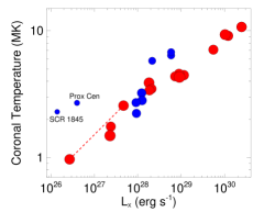
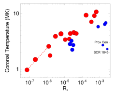
The correlations between hardness ratio and the three measures of X-ray activity are shown in Fig. 1. The red and blue points are for stars above and below 0.65 M_⊙ respectively (repeating this analysis with smaller mass bins leads to the same conclusion). Although there is overlap between the two mass bins in the $L_{\text{X}}$ and $R_{\text{X}}$ distributions, at a given temperature, higher mass stars are clearly likely to have higher values of $L_{\text{X}}$ and lower values of $R_{\text{X}}$ than lower mass stars. On the other hand, the distributions for the two mass bins in the $F_{\text{X}}$ plot overlap excellently, providing a good visual indication that there is one mass-independent relation between $F_{\text{X}}$ and coronal temperature.

3 The Correlation Between X-ray Surface Flux and Coronal Temperature

In this section, we show in a more comprehensive way that there exists one universal relation between coronal temperature and $F_{\text{X}}$ and derive a simple scaling law between the two quantities. For this purpose, we collect coronal temperature estimates from the literature based on multi-temperature emission measure distribution (EMD) fits to high-resolution Chandra and XMM-Newton spectra. Our sample contains 24 stars in total with masses ranging from $\sim$0.1 M_⊙ to $\sim$1.2 M_⊙, including the Sun. For each EMD, we calculate the coronal average temperature by assuming that the logarithm of the average temperature is the emission measure weighted average of the logarithm of the temperatures of each component (Güdel et al. 2007; Johnstone et al. 2014), i.e.

$$\log\bar{T}_{\text{cor}}=\frac{\sum_{i}\text{EM}_{i}\log T_{i}}{\text{EM}_{\text{tot}}},$$ (1)

where the sums are over all measured components of the emission measure distribution with each component having an emission measure of $\text{EM}_{i}$ and a temperature of $T_{i}$, and $\text{EM}_{\text{tot}}=\sum_{i}\text{EM}_{i}$. Stellar radii, $F_{\text{X}}$ values, $\bar{T}_{\text{cor}}$ values, and the references for our sample of stars are given in Table. 1.

We make the assumption that the coronal temperature, stellar mass, and $L_{\text{X}}$ can be related by

$$L_{\text{X}}M_{\star}^{c}=a\bar{T}_{\text{cor}}^{b},$$ (2)

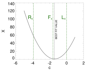
where $a$, $b$, and $c$ are parameters to be fit to the sample. The interesting parameter here is $c$ since its best fit value is dependent on which measure of emission correlates best with coronal temperature. If $L_{\text{X}}$ is the best parameter, then $c\approx 0.0$; if $F_{\text{X}}$ is the best parameter, then $c\approx-1.6$; if $R_{\text{X}}$ is the best parameter, then $c\approx-3.9$. We define our goodness-of-fit parameter, $X$, for a given set of values for $a$, $b$, and $c$, as

$$X=\sum_{i}\gamma_{i}\left[\log\left(L_{\text{X},i}M_{\star,i}^{c}\right)-\log(a)-b\log(T_{i})\right]^{2},$$ (3)

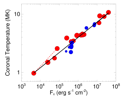
where the sum is over all stars given in Table. 1 and $\gamma_{i}$ is a parameter that we use to weight the importance of certain stars in our fit. In order to make the set of low mass stars have the same importance in our fit as the larger set of higher mass stars, we assume $\gamma_{i}=1$ for all stars with masses above 0.5 M_⊙ and $\gamma_{i}=4$ for all stars with masses below 0.5 M_⊙. To find the value of $c$, we fit the free parameters in Eqn. 2 for each value of $c$ between -5 and 1. In Fig. 2, we show the best fit value of $X$ as a function of $c$. The best fit value of $c$ is -1.45, which shows that coronal temperature correlates with $F_{\text{X}}$ much better than with $L_{\text{X}}$ and $R_{\text{X}}$.

That $F_{\text{X}}$ is better than $L_{\text{X}}$ and $R_{\text{X}}$ can be easily seen in Fig. 3 and is most clear from the two lowest mass stars in the sample, SCR 1845 and Proxima Centauri. Our best fit line in the upper panel of Fig. 3 is given by

$$\bar{T}_{\text{cor}}\approx 0.11F_{\text{X}}^{0.26},$$ (4)

where $\bar{T}_{\text{cor}}$ is in MK and $F_{\text{X}}$ is in erg s^-1 cm^-2. Our result is consistent with the relation provided by Telleschi et al. (2005) for just the solar analogues in the sample. Despite the large range of masses, all of our stars fit this relation excellently, providing confirmation of our conclusion that one universal scaling law exists between $F_{\text{X}}$ and coronal temperature.

4 Conclusions

It is very clear that the emission measure weighted average coronal temperature scales very closely with X-ray surface flux. Our scaling law between $F_{\text{X}}$ and coronal temperature can be used to accurately estimate the coronal average temperature of any low-mass main-sequence star when the value of $F_{\text{X}}$ is known. Alternatively, $F_{\text{X}}$ can be roughly estimated based on the star’s mass and rotation rate (Pizzolato et al. 2003; Wright et al. 2011; Reiners et al. 2014). The scaling law that we derive could be useful as input into coronal models (e.g. Jardine et al. 2002) and stellar wind models that scale wind temperature with coronal temperature (Holzwarth & Jardine 2007; Johnstone et al. 2015a; Johnstone et al. 2015b).

For a star with a given mass and radius, the level of X-ray emission is determined primarily by its rotation rate, with quickly rotating stars emitting more X-rays than slowly rotating stars until a certain threshold where the X-ray emission saturates (Pallavicini et al. 1981; Vilhu 1984). In the unsaturated regime, a star’s X-ray luminosity scales well with its rotation period approximately as $L_{\text{X}}\propto\Omega_{\star}^{2}$ (Reiners et al. 2014), which combined with the assumption that $R_{\star}\propto M_{\star}^{0.8}$, implies that

$$\bar{T}_{\text{cor}}\propto M_{\star}^{-0.42}\Omega_{\star}^{0.52}.$$ (5)

A similar result can be obtained using the scaling laws of Wright et al. (2011). Given that the saturation threshold appears to approximately be at a single mass-independent value of $R_{\text{X}}$, our result implies that in the saturated regime, low-mass stars have cooler coronae than high-mass stars. Assuming $L_{\text{bol}}\propto M_{\star}^{3.9}$ and $R_{\star}\propto M_{\star}^{0.8}$ implies that among saturated stars

$$\bar{T}_{\text{cor}}\propto M_{\star}^{0.6}.$$ (6)

Assuming a saturation Rossby number ($=P_{\text{rot}}/\tau_{\text{c}}$) of 0.13 (Wright et al. 2011) and a convective turnover time given by $\tau_{\text{c}}=15.49\left(M_{\star}/M_{\odot}\right)^{-1.08}$ days (Reiners et al. 2014), the mass dependent satiation threshold is approximately given by

$$\frac{\Omega_{\star}}{\Omega_{\odot}}=13.53\left(\frac{M_{\star}}{M_{\odot}}\right)^{1.08},$$ (7)

where we use $\Omega_{\odot}=2.67\times 10^{-6}$ rad day^-1.

The mass dependence of coronal temperature in the saturated regime is an interesting consequence of the fact that coronal temperature depends on $F_{\text{X}}$ and not $R_{\text{X}}$ and can have consequences for the influence of stellar high-energy radiation on the upper atmospheres of planets. Given that the location of the habitable zone is to first approximation determined by $L_{\text{bol}}$, all planets within the habitable zones around saturated stars should be exposed to approximately the same stellar X-ray and EUV fluxes regardless of the central star’s mass. However, the spectra of high-mass saturated stars is likely to be harder (i.e. more photons at higher energies) than the spectra of low-mass stars. The higher photon energies will mean that the radiation is likely to penetrate deeper into a planetary upper atmosphere, which could lead to differences in the atmospheric photochemistry and mass loss rates.