Simulating Factorization with a Quantum Computer

Abstract.

Modern cryptography is largely based on complexity assumptions, for example, the ubiquitous RSA is based on the supposed complexity of the prime factorization problem. Thus, it is of fundamental importance to understand how a quantum computer would eventually weaken these algorithms. In this paper, one follows Feynman’s prescription for a computer to simulate the physics corresponding to the algorithm of factoring a large number $N$ into primes. Using Dirac transformation theory one translates factorization into the language of hermitical operators, acting on the vectors of the Hilbert space. This leads to obtaining the ensemble of factorization of $N$ in terms of the Euler function $\varphi(N)$, that is quantized. On the other hand, a quantum mechanical prime counting function $\pi_{QM}(x)$, where $x$ factorizes $N$, is derived. This function converges to $\pi(x)$ when $N\gg x$. It has no counterpart in analytic number theory and its derivation relies on semiclassical quantization alone.

I dedicate this paper to Professor Emeritus José Luis Sánchez-Gómez.

1. Introduction

The computational effort required to find the prime factor of a large number $N$ is the basis for the widely used RSA public key encryption system. This makes relevant the study of new methods and algorithms of factorization. The procedures of all classical computers algorithms perform different kind of sieves[1] of the primes $\{x\}\leq N^{1/2}$, but, despite the many mathematical successes, the factorization time of all classical algorithms still scales, at most, sub exponentially in the number of bits of $N=2^{b}$.

Suppose one finds, for some integer $a$, $gcd(a,N)=1$, the period $r(a;N)$ of the function $f(a;z)=a^{z}\ mod\ N,$ $=f(a;z+r)\ mod\ N,$ then one gets the factors $N=x_{+}x_{-}$ simply as

$$x_{\pm}=gcd(a^{r/2\pm 1},N).$$

Shor has found an algorithm that implements the quantum Fourier transform of $f(z)$ yielding to the value of $r$ in polynomial time in a quantum computer [2]. Yet, the current state of the art of quantum computation would not allow for factorization if $N$ is large.

The grounds of quantum computation speed up versus classical computation is the property of entanglement of different states amplitudes (linear superposition) for the output of physical systems (qubits) that represents the logic of the algorithm itself. Moreover, the very principle of quantum computation is Feynman’s observation, describing the problem of simulating quantum physics with computers[3] which, in the end, is equivalent to obtaining a pseudo-probability measure from the unitary evolution of Wigner’s function, calculated for the input states of the computer. Generally speaking, it would involve the whole Hilbert space of the physical system we intend to simulate, and this is the profound difficulty to perform real quantum computations.

Now, following Feynman’s observation, we could ask for the possibility to obtaining the Hilbert space of some (already) quantum computer that performs factorization. This is the approach of the paper, in this case, obtaining the physics from the classical algorithm (conversely to standard quantum computation that requires the realization of a physical system performing the algorithm). These are the grounds and methods of theoretical physics arising from semiclassical quantization of arithmetical functions once they are translated to the language of Hamiltonian mechanics. To this aim, we will transform the number theoretical functional of factorization, described in section 2, precisely into the Jacobi functional defined in the computer coordinates space. It prescribes a methodology based on Dirac-Jordan transformation theory[4] and Feynman’s class of quantum computers (full Hilbert space) in number theory.

Moreover, this could also be consistent with the hypothesis of Hilbert and Pólya (see [5]) related to, more precisely, defending the idea that the the Riemann function $\zeta(s)$ zeros, should be obtained from the spectrum of a suitable Hermitical operator (the Feynman Quantum Computer for Riemann’s $\zeta(s)$) . It amounts to affirm the Riemann hypothesis[6], i.e., for such an Hermitical operator,$H$, the Schrödinger equation,

$$H\psi_{m}(q)=T_{m}\psi_{m}(q)$$

holds in some parametric unbounded space ${q}$ acting on the Hilbert space vectors $\psi_{m}$ and the (real) eigenvalues $T_{m}$ should necessarily correspond to the zeros of $\zeta(s)$ on the critical line $s=1/2+iT_{m}$.

The meaning of the Hilbert space $\{\psi_{m}(q)\}$, parametric space $\{q\}$ and the quantum conditions remains an open question. Some ad hoc ideas dealing with such a Hilbert construction have been proposed so far, the more promising being that of Berry and Keating [7] relating the semiclassical quantization of some yet abstract physical system with the properties of Riemann $\zeta(s)$. In this work we will not follow on these investigations directly, rather we will derive a classical Hamiltonian and the Hilbert construction for the factor $x$ of $N$; this is indirectly related to the theory of primes upon its dependency with the theory of factorization of a number $N$.

Therefore, similarly to those ideas, we intend to directly calculate from the methods of semiclassical quantization the exact values of such a well defined arithmetical function. The Hamiltonian methods and quantum transformation theory are the resources needed to obtain: (1) the dimensionality of the Hilbert space, (2) the semi classical parametric space $\{q\}$ and (3) the unitary state basis $\{\psi_{m}\}$. In the end, quantization amounts to be equivalent to the requirement of divisibility and, in this sense, the discreteness of the factors of an integer $N$ satisfying the limits derived from the definition of the classical Hamiltonian is predicted and modeled. As in standard quantum mechanics, the correspondence principle is required to recover classical number theory. This is modeled upon the detailed calculation of the constants in the integral of the solutions of the quantum conditions.

Our results are those of a Sturn-Liouville problem in quantum mechanics obtaining the factorization ensemble. It leads to a methodology to exhaust all the prime factor candidates of $N$. A proof of the successfulness of the present approach is the arrival to a new expression for the prime counting function $\pi_{QM}(x;N)$, derived from the exact quantum mechanical solution, having no counterpart in number theory, depending on $N$ as a parameter, if $x$ factorizes $N$; the exactitude of this quantum mechanical prime counting function increases indefinitely for large $N$ and it will eventually become a better approximation than $\pi(x)\sim Li(x)$. Indeed,

$$\pi(x)-\pi_{QM}(x;N)\rightarrow 0$$

for $N\gg 1$. This will be the main result of this paper.

If RSA security can be weakened in this way by a quantum computer, one would be led to consider quantum tokens as the alternative to classical network security[8].

2. Prime factorization and Hamiltonian Mechanics

To simulate the computer of factorization we first require the classical theory. In physics what one uses is the Jacobi functional of the system written in canonical coordinates. So, firstly we are obliged to write a kind of functional analogous law to Jacobi’s having the meaning of Euclides’s algorithm for prime factoring $N$

$$\pi(x)\leq\pi(N^{1/2})$$

for the primes candidates $x$.

Now, in order to find how the algorithm works in the computer, we should find how this restricts the set of the $x$ for some input $N$. Recall now that for the input $N$ there are many other $N_{\sigma}$, close enough to $N$ that satisfy $j=\pi(N^{1/2})=\pi(N_{\sigma}^{1/2})$, so $x$ can be a factor of all those $N_{\sigma}$’s in a neighborhood $\mathcal{F}(j)$ of the input $N$. Define now, for $N_{\sigma}\in\mathcal{F}(j)$,

(1) $$E\{j;x_{\sigma}\}=\frac{\pi(x_{\sigma})\pi(N_{\sigma}/x_{\sigma})}{j^{2}}.$$

And $\mathcal{F}(j)=\{N_{\sigma}$; $\pi(N_{\sigma}^{1/2})=j\}$; $x_{\sigma}\cdot y_{\sigma}=N_{\sigma}\in\mathcal{F}(j)$, for the primes $(x_{\sigma},y_{\sigma})$, and $E_{\sigma}$ in Eq. (1) defined in $\mathcal{F}(j)\subset\Pi\{2\}$ ( $\Pi\{2\}$ being the set of all integers having two prime factors).

For some input number $N$, $\mathcal{F}(j)$ would be the factorization ensemble of $N$. Now if for $N_{\sigma}$ integer, we could find another prime $y_{\sigma}=N_{\sigma}/x_{\sigma}$ such that equation (1) obtains a single value of $E_{\sigma}$, then $\mathcal{F}(j)$ defines a proximity of $N$ that exhausts all the prime factor candidates pairs $(x_{\sigma},y_{\sigma})$ of $N$.

Moreover, given that, by definition, $N\in\mathcal{F}(j)$, counting all the $N_{\sigma}$ in $\mathcal{F}(j)$, i.e., finding the cardinality $F(j)$, will obtain the algorithmic complexity of factoring $N$.

Prime Number Theorem obtains how $F(j)=Card\{\mathcal{F}\}$ scales for large N. Let $\pi(N^{1/2})=j$, then, since $\mathcal{F}(j)\subset\Pi\{2\}$,

(2) $$F(j)=\sum_{\pi_{2}(j-1)}^{\pi_{2}(j)}1=\sum_{i=1}^{j-1}[\pi(x(j)^{2}/x_{i})-\pi(x(j-1)^{2}/x_{i})]=f(j+1)-f(j-1)+j,$$

where

$$f(j)=\sum_{i=1}^{j-1}\pi(x(j)^{2}/x_{i})$$

can be computed asymptotically as

$$\rightarrow\sum_{p=2}^{x(j)}\frac{x(j)^{2}}{p(\ln(x(j)^{2}/p)-1)}=\frac{x(j)^{2}}{\ln(x(j)^{2})-1}\{\sum_{p=2}^{x(j)}\frac{1}{p}+\frac{\ln p}{p(\ln(x(j)^{2}/p)-1)}\},$$

now take $x(j)\approx N^{1/2}$; after some straightforward albeit long calculations, replacing the sums by integrals

$$\sum_{p}^{x(j)}f(p)\simeq\int_{2}^{x(j)}\frac{f(y)}{\ln y}dy+\cdots,$$

one gets

(3) $$F(j)\simeq N^{1/2}\cdot(\ln\ln N^{1/2}+C)\cdot\{1-\ln\ln N^{1/2}/\ln N^{1/2}+1/\ln N^{1/2}+\cdots.\}$$

Here $C(N\gg 1)\simeq\ln 2+B_{1},$ where

$$B_{1}=\lim_{L\rightarrow\infty}\sum^{L}1/p-\ln\ln(L)=0.2614972\cdots$$

is Meissel Mertens constant.

Since finding the co-prime $y_{\sigma}$ imposes $\pi(x_{\sigma})\leq\pi(N^{1/2})$ one would expect statistically, as many as $N^{1/2}/x_{\sigma}$possible values of $y_{\sigma}$ per each $x_{\sigma}$ in $\mathcal{F}(j)$.

Hence, we could replace the problem of finding the prime factor $x$ of $N$ with that of solving the more general functional equation

(4) $$E\{j;x_{\sigma}\}=E(N,x)).$$

Now rework Eq. (4) introducing the variables $p$ and $q$.

(5) $$p=\frac{\pi(y_{\sigma})-\pi(x_{\sigma})}{2j}$$

(6) $$q=\frac{\pi(y_{\sigma})+\pi(x_{\sigma})}{2j}.$$

We recast Eq. (4) in the following suggestive way,

(7) $$-p^{2}+q^{2}=E$$

Whose solution is that of a classical inverted harmonic oscillator

$$p=E^{1/2}\sinh(t),$$

$$q=E^{1/2}\cosh(t).$$

For $N>>1$ the functional $E$ is essentially a step function (because for the same value of $x_{\sigma}$ there are about $\sim N^{1/2}/x_{\sigma}$ values of $y_{\sigma}$ with almost the same value of $E$).

Along with the computation of $E$ from Eq.(7), we might have considered variations in $p$ and $q$ due entirely to changes in $t$. Now $t$ is approximately a quasi-continuum parameter at $x<<N^{1/2}$ and, at those conditions, it has the meaning of the time variable in Hamilton’s equations ($E$ an adiabatic invariant in the variation)

(8) $$\delta p=-\partial_{q}H\delta t,$$

(9) $$\delta q=\partial_{p}H\delta t$$

$H$ being the Hamiltonian of the canonical coordinates $p$ and $q$.

(10) $$H(p,q)=\frac{1}{2}(-p^{2}+q^{2}).$$

Moreover $p=\partial_{q}S(q)$, so that a Hamilton-Jacobi condition exists for the functional $S(q)$

(11) $$H(\partial_{q}S(q),q)=E/2;$$

Jacobi’s functional $S(q)$ is the analogous to the number-theoretical functional $E(x^{\prime})$.

Equation (11) is relevant because $q$ is bounded and therefore its solutions are confined trajectories in parametric space.

(12) $$q\leq\frac{\pi(N/2)+\pi(2)}{2\cdot\pi(N^{1/2})}\sim\frac{1}{8}N^{1/2}.$$

$\omega=\partial_{S}H$ would be related to the quasi-period of those confined trajectories and we are led now to the conditions of semiclassical quantization.

3. Quantization

In the $E$ representation, consider the state $\psi_{E}(q)$, that determines the quantum amplitude of probability of a system semiclassically picked precisely on the classical trajectory given by $S(q)$.

The state of the computer is

$$\Psi(q;j)=\sum_{k=1}^{k=F(j)}\frac{1}{F(j)^{1/2}}\psi_{E_{k}}(q)$$

Where the dimension of the Hilbert space of the computer that factorizes $N$ is assumed to be $F(j)$.

Now, the Hamilton-Jacobi constraint for $S(q)$ and quantum transformation theory allow us to obtain the momentum operator acting on the wave functional $\psi_{E}(q)$ for the q-numbers.

(13) $$p\rightarrow-i\partial_{q}$$

The Hamiltonian constraint in Eq. (7) becoming a Hermitical operator in our canonical coordinates acting on $\psi$.  

(14) $$\frac{d^{2}\psi(q)}{dq^{2}}+q^{2}\psi(q)=E\psi(q),$$

Our coordinate space satisfies $E\leq q\leq\ qm(N)$, where $qm(N)<N^{1/2}/8$, therefore, our quantum conditions should be

(15) $$\psi(E^{1/2})=0;$$

(16) $$\psi(qm(N))=0.$$

The dimension of the Hilbert space of $\psi$ is the cardinality of the factorization ensemble, $I\{\mathcal{F}(j)\}$.

The Schrödinger equation (14) and the Sturn-Liouville constraints (15) and (16) define the eigenvalue problem leading to the quantization of $E$ without further assumptions. In this sense, dicreteness of the prime factorization of $N$ is a natural consequence of quantization.

In order to solve equations (14), (15) and (16) one makes $\rho=q^{2}$ and $\psi=\phi/\rho^{1/4}$, obtaining

(17) $$\frac{d^{2}}{d\rho^{2}}\phi+\frac{l(l+1)}{\rho^{2}}\phi+2\mu(r^{2}-\frac{z^{2}}{\rho})\phi=0,$$

where $l=-1/4$, $\mu=1/2$, $r=1/2$ and $z^{2}=E/4$.

That is the 3-dimensional Schrödinger equation for the coulombian scattering of two identical charged particles in their center of mass. Quantum theoretically, the spectrum of $E$ corresponds to the quantization of electricity of some system under the conditions of confinement in (17).

The solution of (17) is asymptotically for $\rho\gg 1$

(18) $$\phi(\rho)\sim\sin(\frac{\rho}{2}-\frac{E}{4}\ln(\rho)+\delta_{Coul}(E)+\delta_{0}(E)),$$

where $\delta_{Coul}(E)=Arg\{\Gamma(-i\frac{E}{4}+\frac{3}{4})\}$ and

(19) $$\delta_{0}(E)=-A\>N^{1/2}\!\ln(E)-h_{1}+o(1/E^{2});$$

$A$ and $h_{1}$ being the two (yet arbitrary) integration constants of our second order differential equation; $\delta_{Coul}(E)$ is a shift in the distorted Coulomb wave for the asymptote while $\delta_{0}$ represents the additional phase drift obtained from the first condition at $\rho=E$, $\phi(E)=0$ using the general solution of (17) [10]

(20) $$\phi(\rho)=\rho^{3/4}e^{-i\rho/2}\{U(\alpha,3/2,i\rho)+\cot\delta_{0}(E)F(\alpha,3/2,i\rho)\}.$$

Here $F(a,b,c)$ and $U(a,b,c)$ are the confluent hypergeometric functions, $\alpha=-i\frac{E}{4}+\frac{3}{4}$.

Now if $\rho\gg 1$

$$F(\alpha,1/2,i\rho)\sim\frac{1}{\Gamma(\alpha)}(i\rho)^{\alpha}\exp(i\rho),$$

and

$$U(\alpha,1/2,i\rho)\rightarrow 0,$$

which directly obtains Eq. (18). Moreover, the logarithmic behavior in $\delta_{0}$ results also from these aymptotics and the fact that,

$$U(\alpha,1/2,iE)\simeq(iE)^{-\alpha}=\exp(i\pi\alpha/2)(1+\ln(E)\alpha+\cdots).$$

The condition $\phi(E)=0$, yields to Eq. (19).

Eq.(19) is the first quantum condition for the confined wave, the second $\phi(N/64)=0$ imposes from (18)

(21) $$\delta_{Coul}(E)+\delta_{0}(E)+N/128-E/4\ln(N/64)=n\pi$$

where $n$ is an integer number.

Redefining $n$ ,

(22) $$n=\left[N/(128\pi)\right]-k,$$

$k$ an integer, $1\leq k\leq F(j)$, also taken into account that for large $E$

(23) $$\delta_{Coul}(E)=Arg\{\Gamma(-i\frac{E}{4}+\frac{3}{4})\}\sim E/4(1-\ln(E/4)+o(1/E^{2})).$$

Define now, for convenience in the notations,

$$\gamma=j/N^{\frac{1}{2}}\ll 1.$$

Ṫhus equation (21) leads asymptotically $N\gg 1$ to

(24) $$\frac{N^{1/2}\gamma}{\pi}\ln(E)\{1-\frac{E(\ln 2-1/2)}{2AN^{1/2}}\}+\frac{E}{2\pi N^{1/2}}(1-\frac{3}{2}\gamma)=\frac{\gamma}{A}(k-h_{1}/\pi)+o(1/E^{2})$$

$$\rightarrow\frac{N^{1/2}}{\pi}\ln(E)=\frac{1}{A}(k-h_{1}/\pi)+o(1/E^{2}).$$

Eq. (24) is the second quantum condition and represents the quantization of $E$. It’s just Bohr-Sommerfeld quantization of the states $\psi_{k}(E;q)$.

Let us see how $E$ scales for $x_{\sigma}\ll N^{1/2}$. The functional of factorization attains its maximum at $\pi(3)=2$,

(25) $$E(x_{\sigma}=3)=2\frac{\pi(N/3)}{j^{2}}\simeq\frac{1}{3\gamma},$$

for $N\gg 1$. Eq. (25) suggests the Ansatz for the Quantum Mechanical Asymptote of the arithmetical functional $E$

(26) $$E_{QM}=E_{1}\cdot\gamma^{\kappa_{1}-\kappa};$$

where

$$\kappa\equiv k/I\leq 1\sim O(1),$$

$$\kappa_{1}\equiv k_{1}/I$$

and $E_{1}=O(1)$ is a constant related to $k_{1}$.

Feeding this back into Eq. (24) one directly obtains the appropriate values of $A$ and $h_{1}$:

$$A\simeq\frac{\pi I}{N^{1/2}\ln(1/\gamma)}=O(1),$$

and

$$h_{1}\simeq\pi k_{1}.$$

Therefore, remarkably, the Ansatz (26) becomes the exact asymptotic solution of (24).

Yet, $k_{1}$ must be determined from consistency with the PNT asymptote of $E$ at large $N$.

Now, in Eq. (1) put $\pi(x)\sim Li(x)$; etc., to obtain another asymptote for $E(x;N)$ if $x=O(N^{1/2})$

(29) $$E_{Li}(N;x)\simeq(1-u(x;N)^{2})^{-1}$$

With the help of the arithmetical function

$$u(x;N)=\gamma\ln(N^{\frac{1}{2}}/x)$$

defined for the prime factor $x$ of $N$.

Moreover, $u$ is related to Euler’s function

(30) $$\varphi(N_{\sigma})=(x_{\sigma}-1)\cdot(N_{\sigma}/x_{\sigma}-1)=N_{\sigma}-2\!N_{\sigma}^{1/2}\cosh(u/\gamma)+1.$$

Now, for $N_{\sigma}\in\mathcal{F}(j)$, $E=f(u)$ is quantized and so are the functions of $u$.Comparing Eqs. (29) and (26), it predicts the existence of a map

$$u(x;N)\leftrightarrow\kappa(j).$$

Moreover, the function

$$(N_{\sigma}^{1/2}-\frac{\varphi(N_{\sigma})}{N_{\sigma}}+N_{\sigma}^{-1/2})=\cosh(u/\gamma),$$

takes discrete values in $\mathcal{F}(j)$.

Technically, in order to derive explicitly $u(\kappa)$, one has to find and solving the Schrödinger equation for $\psi_{\varphi}(q_{\varphi})$, provided the canonical transformations

$$p_{E},q_{E}\rightarrow p_{\varphi},q_{\varphi},$$

Instead of doing this, let’s follow a straightforward approach to obtaining $u(\kappa)$ simply using the known statistics for $N_{\sigma}\in\mathcal{F}(j)$. This can be done upon calculating a minimal (three points) Lagrange Polynomial fit between $\kappa$ and $u$ in our region of interest $u\sim O(1)$ where the approximation $1/E^{2}$ is valid. This amounts to selecting

$$u(3)\approx 1\leftrightarrow\kappa(3)=1-\frac{5/6N^{1/2}}{F(j)},$$

$$u(N^{1/2})=0\leftrightarrow\kappa(N^{1/2})=0$$

and

$$u(2)=\gamma\ln(\frac{N^{1/2}}{2})\leftrightarrow\kappa(2)=1.$$

This being done, it provides asymptotically

(31) $$u(\kappa)=\alpha(N)\kappa-\beta(N)\kappa^{2}$$

where $\alpha$ and $\beta$ are

(32) $$\alpha(N)\simeq 2+O(\gamma\ln 1/\gamma);$$

(33) $$\beta(N)\simeq 1+O(\gamma\ln 1/\gamma).$$

Then,

(34) $$\kappa\simeq\alpha/(2\beta)-1/\beta(\alpha^{2}/4-\beta u)^{1/2}$$

Selecting $E_{1}$ such that $E_{QM}(\kappa_{1})=E_{Li}(u(\kappa_{1}))$ obtains :

(35) $$E_{1}(\kappa_{1})\simeq(1-u(\kappa_{1})^{2})^{-1}.$$

This taken into account, Eq.(26) finally yields to

(36) $$E_{QM}(x;N)=E_{1}(\kappa_{1})\cdot\gamma^{\{1/\beta(\alpha^{2}/4-\beta u(x;N))^{1/2}+\kappa_{1}-\alpha/(2\beta)\}}\;$$

Here $\kappa_{1}$, after Eqs. (28) and (35) is the series

(37) $$\kappa_{1}\simeq(1/6)/\ln(1/\gamma)+R/\ln(1/\gamma)^{2}+O(1/\ln(1/\gamma)^{3})\},$$

and $R=(5/6)C$ is a numerical constant.

4. Prime counting function $\pi_{QM}(x;N)$

Even though (36) is just the solution for $\ln x\ll 1/2\ln N$, by construction it would become exact in its range of validity ($\kappa\geq\kappa_{1}$, say).Then, we might use it to obtain a completely new approximation for the prime counting function $\pi(x)$, i.e., for

$$x<N^{1/2}\exp(-u(\kappa_{1})/\gamma).$$

(38) $$\pi_{QM}(x;N)\equiv E_{QM}(x;N)\frac{\pi(N^{1/2})^{2}}{\pi(N/x)}$$

Recall that $E(x;N)$ can be rewritten simply as

$$E(x;N)=x\frac{\pi(N/x)}{N\gamma}\cdot\frac{\pi(x)}{x\gamma}$$

and since PNT asymptote yields to

$$x\frac{\pi(N/x)}{N\gamma}\simeq\frac{1}{1+u},$$

Eq. (38) obtains

$$\pi_{QM}(x;N)\rightarrow E_{1}\gamma x\;(1+u)E_{QM}(x;N);$$

where $u\simeq 1-\gamma(\ln x-1).$

$\gamma$, $E_{1}$ and $\kappa_{1}$ being known functions of $N$. To derive the explicit formula above we took $\pi(N/x)\sim Li(N/x)$ and $\pi(N^{1/2})\sim Li(N^{1/2})$, for $N\gg 1$.The larger $N$ in (38) the better its exactitude.

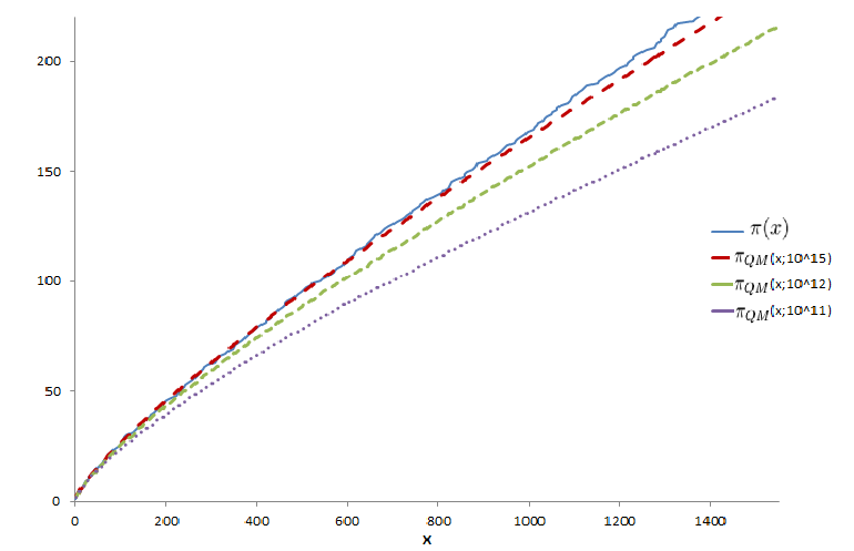
Figure 1. $\pi_{QM}(x;N)$ vs actual $\pi(x)$

Remarkably, in the limit $N\rightarrow\infty$, $\kappa_{1}\rightarrow 0$, and we get $\lim_{j\rightarrow\infty}\mathcal{F}(j)=\Pi\{2\}$.

(39) $$\pi_{QM}(x;N\gg 1)\simeq\pi(x).$$

5. Acknowledgment

This work has been partially supported by Comunidad Autónoma de Madrid, project Quantum Information Technologies Madrid, QUITEMAD+ S2013-IC2801. I thank to Vicente Martín and Jesús Martínez-Mateo for suggestions and assessment.

References

- [1] Pomerance, C. (1996). ”A Tale of Two Sieves”. Notices of the AMS 43 (12). pp. .
- [2] Shor, P.W. “Algorithms for quantum computation: Discrete logarithms and factoring,” in Proceedings 35th Annual Symposium on Foundations of Computer Science, edited by S. Goldwasser (IEEE Computer Society Press, Los Alamitos, CA, 1994), p. 124.
- [3] Feymann R., Inter. J. Mod. Phys. 21,6/7, 1982 pp .
- [4] Dirac, P.A.M. (1933)., Phys.Z. Sowietunion,3, pp 1-10.
- [5] Montgomery, H.L., The pair correlation of zeros of the Riemann z function, Proc. Sympos.Pure Math, 24 1973,pp. .
- [6] Riemann, B. On the Number of Primes Less Than a Given Magnitude. Gesammelte Werke. Teubner, Leipzig, 1892.
- [7] Berry, M.V., and Keating, J.P. The Riemann zeros and eigenvalue asymptotics, SIAM Rev.41(2), 1999 pp. .
- [8] E. Farhi, D. Gosset, A. Hassidim, A. Lutomirski, D. Nagaj, and P. Shor, Physical Review Letters 105, 190503 (2010)
- [9] Bhaduri, R.K., Khare, A., and Law, J. The phase of the Riemann zeta function and the inverted harmonic oscillator. Phys. Rev. E 52 1995,pp. .
- [10] L.D. Landau and E.M. Lifshitz Quantum Mechanics ( Volume 3 of A Course of Theoretical Physics ) Pergamon Press 1965. chapter xVII, pp 526-531 and mathematical appendix pp