The double scaling limit of the multi-orientable tensor model

Abstract

In this paper we study the double scaling limit of the multi-orientable tensor model. We prove that, contrary to the case of matrix models but similarly to the case of invariant tensor models, the double scaling series are convergent. We resum the double scaling series of the two point function and of the leading singular part of the four point function. We discuss the behavior of the leading singular part of arbitrary correlation functions. We show that the contribution of the four point function and of all the higher point functions are enhanced in the double scaling limit. We finally show that all the correlation functions exhibit a singularity at the same critical value of the double scaling parameter which, combined with the convergence of the double scaling series, suggest the existence of a triple scaling limit.

I Introduction

Tensor models (see Rivasseau:2013uca ; review ; Tanasa:2012re for a detailed introduction) generalize matrix models DiFrancesco:1993nw in dimension higher than two. Matrix models posses a $1/N$ expansion David:1984tx ; Kazakov:1985ds dominated by planar graphs Brezin:1977sv and a double scaling limit double ; double1 ; double2 . In this limit one sends $N$ (the matrix size) to infinity and the coupling constant $\lambda$ to some critical value $\lambda_{c}$ in such a way that arbitrary genus surfaces contribute to a $2r-$point function. This is achieved if one keeps the double scaling parameter $N^{\frac{5}{4}}(\lambda_{c}-\lambda)$ fixed. As in this regime all the topologies contribute, the double scaling limit corresponds to a theory at finite Newton coupling EDTDavid . It should be emphasized that, in the case of matrices, the double scaling series are divergent DiFrancesco:1993nw .

Tensor models review generalize matrix models in higher dimension. They posses a $1/N$ expansion (where $N$ is now the tensor size) expansion3 ; expansioin5 and reach a continuum limit review by tuning to criticality. The $1/N$ expansion of tensor models is indexed by the degree, which, contrary to the genus, is not a topological invariant.

Tensor models fall into two broad categories: the invariant models uncoloring which exist for tensors of arbitrary rank and the multi-orientable (MO) one Tanasa:2011ur . While the MO model exists only for tensors of rank three, it exhibits a richer combinatorics than the invariant models in rank three: the class of graphs the MO model sums over is strictly larger than the one the invariant models sum over. In particular, for the multi-orientable model the degree is a halfinteger, while it can only be an integer for the invariant models.

The double scaling limit has recently been studied for the invariant tensor models DGR ; Bonzom:2014oua ; GurSch . It has been found that, denoting $D\geq 3$ the rank of the tensor, the appropriate double scaling parameter is $N^{D-2}(\lambda_{c}-\lambda)$ for $D<6$ and $N^{\frac{2}{3}D}(\lambda_{c}-\lambda)$ for $D\geq 6$. The double scaling series are convergent for $D<6$ and divergent (as they are for matrices) for $D\geq 6$.

In order to identify what features of the double scaling limit of tensor models are robust, we study in this paper the double scaling limit of the MO model. As this model sums over a larger family of graphs than the invariant models in rank three, it is the ideal testing ground for this study. We find that, as it was the case for the invariant models in rank three, the double scaling series in the MO model are convergent. We perform below the analytic resummation of these series for the two point function, the leading singular part of the four point function, and discuss the leading singular part of arbitrary correlation functions. Surprisingly, although the convergence of the double scaling series is robust, the double scaling parameter is not. We show that for the MO model the appropriate double scaling parameter is $N^{\frac{1}{2}}(\lambda_{c}-\lambda)$, hence scales with an exponent of $N$ different from the one of the invariant models in rank three.

Finally, we show that all the (leading singular parts of the) correlation functions become critical at the same critical value of the double scaling parameter and discuss the consequences of this behavior.

II The multi-orientable tensor model

Let $\phi_{ijk}$, $i,j,k=1,\ldots,N$, be the components of a rank three complex tensor $\phi$. The action of the MO tensor model is expansioin5 :

$$S[\phi]=\sum_{ijk}\phi_{ijk}\bar{\phi}_{ijk}-\frac{\lambda}{2N^{3/2}}\sum_{\genfrac{}{}{0.0pt}{}{ijk}{lmn}}\phi_{ijk}\bar{\phi}_{mlk}\phi_{mjn}\bar{\phi}_{iln}\;,$$ (1)

where the scaling with $N$ of the interaction term above is chosen in order for the model to admit a $1/N$ expansion expansioin5 .

The partition function of the MO model:

$$Z=\int\mathcal{D}[\phi]e^{-S[\phi]}\;,\;\;\displaystyle\mathcal{D}[\phi]=\prod_{ijk}\frac{{\rm d}\phi_{ijk}{\rm~{}d}\bar{\phi}_{ijk}}{2\pi\imath}\;,$$

writes in perturbation theory as a sum over Feynman multi-orientable graphs Tanasa:2011ur . The vertices of the MO graphs are four valent, the edges are oriented from $\phi$ to $\bar{\phi}$ and the orientations alternate around a vertex. The edges can be represented as three parallel strands (one for each index of the tensor) and the vertices as the intersection of four half edges such that every pair of half edges share a strand. This leads to the representation in Fig. 1.

Figure 1: An MO vacuum (Feynman) graph.

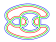
The strands are divided into three classes: the ones in the middle of the edges, called the $S$ (for straight) strands, the ones on the right (with respect to the $\phi\to\bar{\phi}$ orientation) of the edges, called the $R$ (for right) strands and the ones on the left of the edges, called the $L$ (for left) strands. At a vertex the $S$ ($R$ or $L$) strands only connect to $S$ ($R$ or $L$) strands.

To any MO graph one can associate three canonical ribbon graphs, called the jackets, obtained by erasing throughout the graph all the strands in the same class ($S$, $L$ or $R$). For the graph of Fig. 1 for example this leads to the three jackets represented in Fig. 2.

Figure 2: The three jackets associated to the graph of Fig. 1.

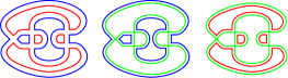
Crucially, the jackets of the MO graphs can be non-orientable (dual to non orientable surfaces). This is a fundamental difference between the MO model and the invariant models.

The degree $\delta({\cal G})$ of a connected MO graph ${\cal G}$ is the half sum of the non orientable genera of its three jackets. It is therefore a positive half integer.

The Feynman amplitude of the graph ${\cal G}$ is expansioin5 $\mathcal{A}(\mathcal{G})=\lambda^{v({\cal G})}N^{3-\delta({\cal G})},$ where $v({\cal G})$ is the number of vertices of ${\cal G}$. The free energy, which is a sum over connected graphs, admits the $1/N$ expansion:

$$\ln Z=\sum_{\mathcal{G}}\mathcal{A}(\mathcal{G})=\sum_{\delta\in\mathbb{N}/2}N^{3-\delta}\Big{(}\sum_{\mathcal{G}|\delta(\mathcal{G})=\delta}\lambda^{v(\mathcal{G})}\Big{)}\;.$$

In the sequel we will use a simplified representation of the MO graphs (introduced in Fusy:2014rba ) as graphs with oriented edges.

III Correlation functions

Let us denote $\Braket{\bar{\phi}\dots\phi\dots}_{c}$ the connected correlation functions of the MO model. The action in Eq. (1) is invariant under the field transformation:

$$\phi^{\prime}_{i_{1}j_{1}k_{1}}=\sum_{ijk}U^{R}_{i_{1}i}O^{S}_{j_{1}j}U^{L}_{k_{1}k}\phi_{ijk}\;,$$

$$\bar{\phi}^{\prime}_{i_{1}j_{1}k_{1}}=\sum_{ijk}\bar{U}^{R}_{i_{1}i}O^{S}_{j_{1}j}\bar{U}^{L}_{k_{1}k}\phi_{ijk}\;,$$

where $U^{R}$ and $U^{L}$ are two (distinct) complex unitary matrices and $O^{S}$ is a real orthogonal matrix. The indices $S$ are special: one must use an orthogonal transformation because the quadratic part contracts and index $S$ of a field $\phi$ with an index $S$ of a field $\bar{\phi}$ while the interaction contracts two indices $S$ belonging either both to fields $\phi$ or both to fields $\bar{\phi}$.

This invariance constrains the correlation functions: averaging over the unitary and orthogonal groups ColSni one finds that the indices of any correlation function must be pairwise identified. For the $R$ and $L$ indices, an index of a $\phi$ must be identified with an index of a $\bar{\phi}$, while for the $S$ indices any pairing is allowed. Thus:

$$\Braket{\bar{\phi}_{\bar{a}\bar{b}\bar{c}}\phi_{abc}}_{c}=\delta^{\bar{a}}_{a}\delta^{\bar{b}}_{b}\delta^{\bar{c}}_{c}\;\mathfrak{K}_{2}\;,$$ (2)

twelve pairings are allowed (see Fig. 3) for a four point function and $2^{-r}r!(2r)!$ pairings for a $2r$ point function.

Figure 3: The twelve index pairings of the four point function.

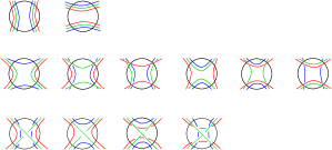
Out of these pairings, $r!$ correspond to a pairing of the external legs (the top row in Fig. 3):

$$\Braket{\prod_{i=1}^{r}\bar{\phi}_{\bar{a}_{i}\bar{b}_{i}\bar{c}_{i}}\phi_{a_{i}b_{i}c_{i}}}_{c}=$$ (3)

$$\qquad=\mathfrak{K}^{(1)}_{2r}\sum_{\sigma}\prod_{i=1}^{r}\delta^{\bar{a}_{i}}_{a_{\sigma(i)}}\delta^{\bar{b}_{i}}_{b_{\sigma(i)}}\delta^{\bar{c}_{i}}_{c_{\sigma(i)}}+\dots\;,$$ (4)

where $\sigma$ runs over permutations of $r$ elements.

The two point function is related to $\ln Z$ by the Schwinger Dyson equation:

$$0=\frac{1}{Z}\int\mathcal{D}[\phi]\sum_{abc}\frac{\partial\left(\phi_{abc}\;e^{-S[\phi]}\right)}{\partial\phi_{abc}}\Rightarrow$$

$$\qquad\Rightarrow\mathfrak{K}_{2}=1+N^{-3}2\lambda\partial_{\lambda}\ln Z\;.$$

This equation is interpreted as follows: $\ln Z$ is a sum over graphs and $\partial_{\lambda}$ acting on $\ln Z$ marks a vertex. Together with the factor $2$ this comes to marking one of the edges incoming at the vertex and $\mathfrak{K}_{2}$ is a sum over MO graphs rooted at an edge, ${\cal G}^{\times}$:

$$\mathfrak{K}_{2}=1+\sum_{\delta\in\mathbb{N}/2}N^{-\delta}\Big{(}\sum_{{\cal G}^{\times}|\delta({\cal G}^{\times})=\delta}\lambda^{v(\mathcal{{\cal G}^{\times}})}\Big{)}\;.$$ (5)

The constant term $1$ represents the ring graph consisting in the root edge closed onto itself and can be included in the sum. The ring graph has three faces, one edge and no vertex hence it has degree zero.

Equation (5) can also be understood as follows. Let us denote $(\bar{\phi}\phi)$ the invariant $\sum_{abc}\bar{\phi}_{abc}\phi_{abc}$. The expectation $\braket{(\bar{\phi}\phi)}_{c}$ is precisely a sum over connected MO graphs having a special edge corresponding to the insertion $(\bar{\phi}\phi)$ which is taken as root. Eq. (2) leads to $N^{3}\mathfrak{K}_{2}=\braket{(\bar{\phi}\phi)}_{c}$ and Eq. (5) follows.

Similarly, $\Braket{(\bar{\phi}\phi)^{r}}_{c}$ is a sum over graphs with $r$ root edges and Eq. (3) leads to:

$$\Braket{(\bar{\phi}\phi)^{r}}_{c}=\mathfrak{K}^{(1)}_{2r}\Big{(}N^{3r}+O(N^{3r-1})\Big{)}+\dots\;.$$

IV Classification by degree

We first discuss graphs with a unique root edge. Let us call a fundamental submelon of ${\cal G}^{\times}$ a subgraph consisting in two vertices connected by three non-root edges such that the two vertices belong to three faces of length two. The degree of ${\cal G}^{\times}$ does not change if one replaces a fundamental submelon by an edge. The melonic graphs critical are the graphs which reduce to the ring graph by eliminating iteratively all the fundamental submelons (see Fig. 4) and therefore have degree zero.

Figure 4: Melonic graphs.

It turns out that the converse is also true critical : a graph has degree zero if and only if is it is melonic. The generating function of rooted melonic graphs with respect to the number of vertices, $T(\lambda^{2})$, obeys the equation:

$$T(\lambda^{2})=1+\lambda^{2}[T(\lambda^{2})]^{4}\;.$$

Cores

Deleting iteratively all the fundamental submelons a graph ${\cal G}^{\times}$ reduces to its core $\hat{\cal G}^{\times}$. The core of the melonic graphs is the ring graph. The set of all the cores consists in all the MO graphs having no fundamental submelon.

Of course there are many graphs corresponding to the same core and the sum over graphs can be reorganized by cores: $\sum_{{\cal G}^{\times}}\lambda^{v({\cal G}^{\times})}=\sum_{\hat{\cal G}^{\times}}\left(\sum_{{\cal G}^{\times}\text{ with core }\hat{\cal G}^{\times}}\lambda^{v({\cal G}^{\times})}\right)$. The graphs corresponding to a core are obtained by inserting melonic graphs on the edges of the core:

$$\sum_{{\cal G}^{\times}\text{ with core }\hat{\cal G}^{\times}}\lambda^{v({\cal G}^{\times})}=\lambda^{v(\hat{\cal G}^{\times})}\left[T(\lambda^{2})\right]^{2v(\hat{\cal G}^{\times})+1}\;,$$

where we accounted for insertions of melonic graphs at both ends of the root edge of the core.

Schemes

The classification of graphs in terms of cores is not sufficient because there are still an infinite number of cores of the same degree.

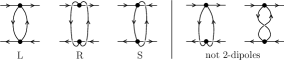
Let us call a dipole a sub graph made of two vertices connected by two non-root edges such that the two vertices belong to exactly one face of length two. As the face of length two can be of type $L$, $R$ or $S$, there are three types of dipoles, depicted in Fig. 5. The dipoles can join together into chains of dipoles. A chain is called broken (and denoted $B$) if the dipoles in the chain are not of the same type and unbroken if they are. The unbroken chains can be $R$, $L$, or $S$ and the unbroken chains of type $S$ are further classified into those with an odd number of dipoles, $S_{o}$, and those with an even number of dipoles, $S_{e}$.

Figure 5: The three types of dipoles, on the left. On the right, subgraphs which are not dipoles.

Replacing a chain of dipoles by a chain of the same type but having a different number of dipoles does not change the degree of a graph. This is why the number of cores of the same degree is infinite. In order to classify the graphs with the same degree into only a finite number of classes one needs to gather in the same class all the cores which only differ by the length of the chains of dipoles. Such a class is represented by a scheme, which is a rooted MO graph with no fundamental submelons and no chains of dipoles, but having, on top of the usual $\lambda$ vertices, five kinds of chain vertices representing the five kinds of chains: $B,R,L,S_{o},S_{e}$.

Let us denote $U(\lambda^{2})=\lambda^{2}[T(\lambda^{2})]^{4}$ the generating function of nonempty melonic graphs. We denote $v$ the total number of usual vertices and $c$, $b$, $s$ and $s_{o}$ the total numbers of chain vertices, broken chain vertices, straight chain vertices and straight odd chain vertices in a scheme. The generating function of rooted MO graphs corresponding to the scheme $S$ is Fusy:2014rba :

$$F_{S}^{(\delta)}(\lambda)=\frac{T(\lambda^{2})6^{b}[U(\lambda^{2})]^{\frac{v}{2}+2c+s_{o}}}{[1-U(\lambda^{2})]^{c-s}[1-U(\lambda^{2})^{2}]^{s}[1-3U(\lambda^{2})]^{b}}\;.$$

Graphs with $r$ root edges are dealt with identically. They are classified by schemes with $r$ roots and the generating function of graphs with $r$ roots corresponding to a scheme with $r$ roots is:

$$F_{S}^{(\delta),r}(\lambda)=\frac{T(\lambda^{2})^{r}6^{b}[U(\lambda^{2})]^{\frac{v}{2}+2c+s_{o}}}{[1-U(\lambda^{2})]^{c-s}[1-U(\lambda^{2})^{2}]^{s}[1-3U(\lambda^{2})]^{b}}\;.$$

The main gain in classifying MO graphs by schemes is that the set ${\cal S}_{\delta,r}$ of the schemes of degree $\delta$ with $r$ roots is finite Fusy:2014rba .

V Dominant schemes

The generating function of rooted melonic graphs becomes critical for $\lambda^{2}_{c}=3^{3}/2^{8}$. In this regime:

$$T(\lambda^{2}) \sim\frac{1}{3}\left(4-\sqrt{\frac{8}{3}}\sqrt{1-\frac{\lambda^{2}}{\lambda_{c}^{2}}}\right)\;,$$

$$1-3U(\lambda^{2}) \sim\sqrt{\frac{8}{3}}\left(1-\frac{\lambda^{2}}{\lambda_{c}^{2}}\right)^{1/2}\;.$$

The generating functions of graphs corresponding to a scheme $F_{S}^{(\delta),r}(\lambda)$ (and consequently the ones of graphs of fixed degree) become singular. The leading singular behavior is given by the schemes which maximize the number of broken chains at fixed degree $\delta$, which we call dominant.

The deletion of a chain vertex consists in deleting the chain vertex and joining the two pairs of half edges at the same end of the chain vertex into two new edges. A chain vertex is called separating if by deleting it the scheme separates into two connected components and non separating if not.

It can be shown Fusy:2014rba that by deleting a non separating chain vertex the degree of a scheme strictly decreases, while by deleting a separating chain vertex the degree of the scheme is distributed among the connected components. It follows that all the chain vertices in a dominant scheme must be separating, and (so as to maximize the number of broken ones) all of them must be broken.

The dominant schemes have then the structure of an abstract tree whose edges represent the broken chain vertices and whose vertices represent the MO graphs obtained by deleting simultaneously all the broken chain vertices. The tree is binary so as to maximize the number of broken chain vertices

The three valent nodes of the tree represent MO graphs of degree zero (otherwise one can build a binary tree representing a scheme with strictly smaller degree by replacing such a node by a MO graph of degree zero). There are four possible graphs: either the ring graph or three melonic graphs with two vertices.

The univalent nodes of the tree can be of two types: they either represent a ring graph consisting in a root edge or they represent a MO graph with exactly one vertex and two edges (a “double tadpole graph”Fusy:2014rba ) which has degree $1/2$. There are two possible double tadpole graphs. The structure of a dominant scheme with several roots is then presented in Fig. 6 below.

Figure 6: A dominant scheme

The dominant schemes with $r$ root edges contribute to the $2r-$point function. As all the chain vertices in such a scheme are broken, the dominant schemes contributed only to $\mathfrak{K}^{(1)}_{2r}$.

The set of dominant schemes with degree $\delta$ and $r$ roots, ${\cal S}^{\text{dom}}_{\delta,r}$, consists in binary trees with $r$ univalent root vertices and another $2\delta$ univalent vertices. Such trees have $2\delta+r-2$ three valent internal vertices and $4\delta+2r-3$ edges. The leading singular contribution to the $2r-$point function is then:

$$\mathfrak{K}^{(1)\text{sing}}_{2r}=N^{3(1-r)}\sum_{\delta\in\mathbb{N}/2}N^{-\delta}\sum_{S\in{\cal S}^{\text{dom}}_{\delta,r}}$$ (6)

$$\qquad T(\lambda^{2})^{r}[2^{2}U(\lambda^{2})]^{\delta}[1+3U(\lambda^{2})]^{2\delta+r-2}\times$$ (7)

$$\qquad\times\left(\frac{6[U(\lambda^{2})]^{2}}{[1-U(\lambda^{2})][1-3U(\lambda^{2})]}\right)^{4\delta+2r-3}\;,$$ (8)

where for the two point function ($r=1$) one needs to add the contribution $T(\lambda^{2})$ of the degenerate dominant scheme consisting in a unique root vertex.

VI The double scaling limit

In the double scaling limit one compensates the $1/N$ suppression of the higher order terms in the series in Eq. (6) by the enhancement at criticality due to the $[1-3U(\lambda^{2})]^{-1}$ factors. This is achieved by sending at the same time $N$ to infinity and $\lambda$ to criticality while keeping the double scaling parameter

$$N^{\frac{1}{2}}\left(1-\frac{\lambda^{2}}{\lambda_{c}^{2}}\right)\equiv\kappa^{-1}\;,$$

fixed. In the double scaling regime we get:

$$T(\lambda^{2})\sim\frac{4}{3}\left(1-\sqrt{\frac{1}{6\kappa\sqrt{N}}}\right)\;,1-3U(\lambda^{2})\sim\sqrt{\frac{8}{3\kappa\sqrt{N}}}.$$

The two point function

The dominant schemes are rooted binary trees which are counted by the Catalan numbers: there are ${\rm Cat}_{n-1}$ such trees with $n-1$ three valent vertices, hence with $n$ non root univalent vertices. The degree of the scheme is $\delta=n/2$ and taking into account the contribution of the degenerate scheme consisting in a unique root vertex we obtain:

$$\mathfrak{K}^{\text{sing}}_{2}=T(\lambda^{2})+\sum_{n\geq 1}{\rm Cat}_{n-1}\frac{1}{N^{\frac{n}{2}}}\times$$

$$\qquad\times T(\lambda^{2})[2^{2}U(\lambda^{2})]^{\frac{n}{2}}[1+3U(\lambda^{2})]^{n-1}$$

$$\qquad\times\left(\frac{6[U(\lambda^{2})]^{2}}{[1-U(\lambda^{2})][1-3U(\lambda^{2})]}\right)^{2n-1}$$

$$=T(\lambda^{2})\left(1+\frac{1}{N^{1/2}}\frac{12\cdot U(\lambda^{2})^{5/2}}{[1-U(\lambda^{2})][1-3U(\lambda^{2})]}\times\right.$$

$$\;\;\times\left.\sum_{n\geq 0}{\rm Cat}_{n}\left(\frac{1}{N^{1/2}}\frac{72\cdot U(\lambda^{2})^{9/2}[1+3U(\lambda^{2})]}{[1-U(\lambda^{2})]^{2}[1-3U(\lambda)]^{2}}\right)^{n}\right)\;,$$

which in the double scaling limit becomes:

$$\mathfrak{K}^{DS}_{2} =\frac{4}{3}\left(1-\sqrt{\frac{1}{6\kappa\sqrt{N}}}\right)+$$

$$\qquad+\frac{4}{3}\frac{1}{N^{\frac{1}{4}}}\sqrt{\frac{\kappa}{2}}\sum_{n\geq 0}{\rm Cat}_{n}\left(\kappa\frac{\sqrt{3}}{2}\right)^{n}$$

$$=\frac{4}{3}\left(1-\frac{\sqrt{1-2\sqrt{3}\kappa}}{N^{\frac{1}{4}}\sqrt{6\kappa}}\right)\;,$$

where the sum over $n$ converges for $\kappa<2^{-1}3^{-\frac{1}{2}}$.

The four point function

The dominant schemes are binary trees with two roots. There are again ${\rm Cat}_{n-1}$ such trees with $n-1$ three valent vertices, but this time they have $n-1$ non root univalent vertices and degree $\delta=\frac{n-1}{2}$. We obtain:

$$\mathfrak{K}^{(1)\text{sing}}_{4}=N^{-3}\sum_{n\geq 1}{\rm Cat}_{n-1}\frac{1}{N^{\frac{n-1}{2}}}$$

$$\quad T(\lambda^{2})^{2}[2^{2}U(\lambda^{2})]^{\frac{n-1}{2}}[1+3U(\lambda^{2})]^{n-1}\times$$

$$\quad\times\left(\frac{6[U(\lambda^{2})]^{2}}{[1-U(\lambda^{2})][1-3U(\lambda^{2})]}\right)^{2(n-1)+1}$$

$$= N^{-3}T(\lambda^{2})^{2}\left(\frac{6[U(\lambda^{2})]^{2}}{[1-U(\lambda^{2})][1-3U(\lambda^{2})]}\right)\times$$

$$\sum_{n\geq 0}{\rm Cat}_{n}\left(\frac{1}{N^{1/2}}\frac{72\cdot U(\lambda^{2})^{9/2}[1+3U(\lambda^{2})]}{[1-U(\lambda^{2})]^{2}[1-3U(\lambda)]^{2}}\right)^{n}\;.$$

In the double scaling limit this becomes

$$\mathfrak{K}^{(1)DS}_{4}=N^{-3+\frac{1}{4}}\sqrt{\kappa}\frac{8\sqrt{3}}{9\sqrt{2}}\left(\frac{1-\sqrt{1-2\sqrt{3}\kappa}}{\sqrt{3}\kappa}\right)\;.$$

Observe that $\mathfrak{K}^{(1)DS}_{4}$ is enhanced by a factor $N^{\frac{1}{4}}$ with respect to the natural $N$ scaling of $\mathfrak{K}^{(1)}_{4}$. This is a consequence of the fact that the singularity of the generating function of dominant schemes boosts this four point function in double scaling.

The $2r-$point function

The dominant schemes are binary trees with $r$ roots and the double scaling limit of $\mathfrak{K}^{(1)}_{2r}$ is:

$$\mathfrak{K}^{(1)DS}_{2r}\sim N^{3(1-r)}N^{\frac{1}{4}(2r-3)}f_{2r}(\kappa)\;,$$

for some function $f_{2r}$ depending only on the double scaling parameter $\kappa$. As it was the case for the four point function, the higher point functions are also boosted in double scaling with respect to their natural scaling in $N$. All the functions $f_{2r}(\kappa)$ are convergent for $2\sqrt{3}\kappa<1$ and exhibit a square root singularity at the critical double scaling coupling $\kappa_{c}=2^{-1}3^{-\frac{1}{2}}$.

VII Towards a triple scaling limit

The results of the previous section open up the possibility to explore a triple scaling regime in which one sends $N\to\infty$, $\lambda\to\lambda_{c}$ such that $\kappa=\left[N^{\frac{1}{2}}\left(1-\frac{\lambda^{2}}{\lambda_{c}^{2}}\right)\right]^{-1}$, instead of being fixed, also goes to criticality $\kappa\to\kappa_{c}=2^{-1}3^{-1/2}$ such that the triple scaling constant $N^{\alpha}(\kappa-\kappa_{c})=x$, with an appropriate choice of $\alpha$, is kept fixed. In this regime the double scaled two point function itself becomes critical and, for a suitable triple scaling exponent $\alpha$, one expects an even larger family of graphs to contribute.

References

- (1) V. Rivasseau, “The tensor track, III,” arXiv:1311.1461 [hep-th].
- (2) R. Gurau and J. P. Ryan, “Colored tensor models - a review,” SIGMA 8 (2012) 020, arXiv:1109.4812 [hep-th].
- (3) A. Tanasa, “Combinatorics of random tensor models,” arXiv:1203.5304 [math.CO].
- (4) P. Di Francesco, P. H. Ginsparg, and J. Zinn-Justin, “2-D Gravity and random matrices,” Phys. Rept. 254 (1995) 1–133, arXiv:hep-th/9306153 [hep-th].
- (5) F. David, “Planar diagrams, two-dimensional lattice gravity and surface models,” Nucl. Phys. B257 (1985) 45.
- (6) V. A. Kazakov, “Bilocal regularization of models of random surfaces,” Phys. Lett. B150 (1985) 282–284.
- (7) E. Brezin, C. Itzykson, G. Parisi, and J. B. Zuber, “Planar diagrams,” Commun. Math. Phys. 59 (1978) 35.
- (8) E. Brezin and V. A. Kazakov, “Exactly solvable field theories of closed strings,” Phys. Lett. B236 (1990) 144–150.
- (9) M. R. Douglas and S. H. Shenker, “Strings in less than one-dimension,” Nucl. Phys. B335 (1990) 635.
- (10) D. J. Gross and A. A. Migdal, “Nonperturbative two-dimensional quantum gravity,” Phys. Rev. Lett. 64 (1990) 127.
- (11) F. David, “Simplicial quantum gravity and random lattices,” arXiv:hep-th/9303127 [hep-th].
- (12) R. Gurau, “The complete 1/N expansion of colored tensor models in arbitrary dimension,” Annales Henri Poincare 13 (2012) 399–423, arXiv:1102.5759 [gr-qc].
- (13) S. Dartois, V. Rivasseau, and A. Tanasa, “The 1/N expansion of multi-orientable random tensor models,” arXiv:1301.1535 [hep-th].
- (14) V. Bonzom, R. Gurau, and V. Rivasseau, “Random tensor models in the large N limit: Uncoloring the colored tensor models,” Phys. Rev. D85 (2012) 084037, arXiv:1202.3637 [hep-th].
- (15) A. Tanasa, “Multi-orientable Group Field Theory,” J.Phys. A45 (2012) 165401, arXiv:1109.0694 [math.CO].
- (16) S. Dartois, R. Gurau, and V. Rivasseau, “Double scaling in tensor models with a quartic interaction,” JHEP 1309 (2013) 088, arXiv:1307.5281 [hep-th].
- (17) V. Bonzom, R. Gurau, J. P. Ryan, and A. Tanasa, “The double scaling limit of random tensor models,” JHEP 1409 (2014) 051, arXiv:1404.7517 [hep-th].
- (18) R. Gurau and G. Schaeffer, “Regular colored graphs of positive degree,” arXiv:1307.5279 [math.CO].
- (19) E. Fusy and A. Tanasa, “Asymptotic expansion of the multi-orientable random tensor model,” arXiv:1408.5725 [math.CO].
- (20) B. Collins and P. Sniady, “Integration with respect to the Haar measure on unitary, orthogonal and symplectic group,” Commun. Math. Phys. 264 (2006) 773, arXiv:0402073 [math-ph].
- (21) V. Bonzom, R. Gurau, A. Riello, and V. Rivasseau, “Critical behavior of colored tensor models in the large N limit,” Nucl. Phys. B853 (2011) 174–195, arXiv:1105.3122 [hep-th].