Randomized migration processes between two epidemic centers

Abstract

Epidemic dynamics in a stochastic network of interacting epidemic centers is considered. The epidemic and migration processes are modelled by Markov’s chains. Explicit formulas for probability distribution of the migration process are derived. Dependence of outbreak parameters on initial parameters, population, coupling parameters is examined analytically and numerically. The mean field approximation for a general migration process is derived. An approximate method allowing computation of statistical moments for networks with highly populated centres is proposed and tested numerically.

Igor Sazonov^a and Mark Kelbert^b,c

^a College of Engineering, Swansea University, Singleton Park, SA2 8PP, U.K.

^b National Research University Higher School of Economics, Moscow, R.F.

^c Department of Mathematics, Swansea University, Singleton Park, SA2 8PP, U.K.

Key words: spatial epidemic models; migration dynamics; ourbreak time

AMS subject classification: 92D30, 91B70, 91B72

Introduction

Epidemic outbreak in a populated center or in a network of populated centra develops stochastically due to random interaction between individuals inside a center and due to a random migration between centers of the network. Conventionally, an epidemic outbreak in a highly populated center is described by deterministic processes in according with Law of Large Numbers (LLN) [2]. The mean field approximation (hydrodynamic limits) of the appropriate statistical models establishes the basic relation of stochastic description to the dynamical equations, say the SIR model (susceptible/infected/ removed) and its more sophisticated modifications (SEIR, SIS, MSIR, etc.)

However, there are two important cases when stochastic effects are essential. Firstly, it is obviously important when the populations in centers are not large. The second less obvious scenario can occur at the initial stage of outbreak when the number of infectives is small, then the discreteness of population can essentially affect the dynamics of the outbreak making it stochastic. For an isolated center, this case is thoroughly studied in [3]. Analysis of a network of interacting epidemic centers requires an account of migration fluxes between them.

So, if the initial number of infectives triggering the outbreak in a particular populated center is small (that is typical for many outbreaks) than the LLN fails at least at initial stage until the number of infectives is large enough. For this reason the observed number of infectives can be significantly different from the prediction of a deterministic model, i.e. the standard deviation of the number of infectives and the peak outbreak time can be wide even in highly populated center or a network of such centers.

In principle, the probability density function (PDF), its standard deviation, and other important characteristics for the outbreak forecast could be determined by a direct numerical simulation. However, this simulation may be very costly and require too much CPU time even for modern computers. Our goal is to develop a technique for a rough estimation of the outbreak statistical characteristics skipping such huge computation by applying some perturbation methods.

Our toolkit is the so-called small initial contagion (SIC) approximation for the case of a large populated center when initial number of infectives is small, cf. [3] in the case of a single populated center. For a network of highly populated SIR centers in the framework of deterministic model such technique is described in [4, 5]. In this paper we develop a stochastic version of SIC approach based on the assumption that in the real epidemic centra the number of infectives triggering an outbreak is still small. In a sense, the SIC approach looks like a key to solving cumbersome epidemic networks.

In [3], a randomized analogue of the standard SIR model is considered. In the SIC approximation, one distinguishes two linked stages of epidemic evolution. At the stage 1 of initial contamination the number of infectives is small and a discrete formulation is vital. At this stage the system is randomized, and governed by stochastic equations. At the stage 2 of developed outbreak when the numbers of individuals in all the components are large the LLN works and the standard deterministic SIR model can describe the outbreak process accurately enough. Therefore it is natural to consider a deterministic system with randomized initial conditions linked to the stochastic stage 1. The statistical characteristics of the complete model are obtained by applying deterministic equations with random initial conditions using the matching asymptotic expansions technique (cf. [6]). In contrast to the traditional technique, the asymptotic approximation of a randomized evolution (at a brief initial period) is matched with a deterministic evolution with randomized initial conditions (for all other times). Nevertheless, as in the traditional approach, we match the approximations at some intermediate time $t$ in the interval where the both approximations are valid and which drops out from the final results (cf. [6]).

The Markov chain (MC) describing the randomized SIR model has been studied previously, e.g., in [7] where a partial differential equation (PDE) for the moment generating function was derived. We develop a similar approach for a pair of linked centers and obtain approximate formulae for their main statistical characteristics. The results of large-scale numerical simulation are in a good agreement with the appropriate models.

The paper is organized as follows. In Section 1 we introduce a MC model describing randomized epidemic outbreak in two populated centers coupled by a random migration of all types of species. Here we consider convergence of this model to a deterministic mean-field model proposed in [8]. In Section 2 we describe a model of random migration between two interacting SIR centers taking place before the outbreak started to determine all the initial conditions for the MC model. Migration between centers is also described as a Markov chain. Here we derive the Master/Kolmogorov’s equations for the probability generating functions (PGF) and solve them analytically. This analysis confirms the diffusion-like model of migration heuristically proposed in [8]. In Section 3 the numerical algorithm for direct solving the MC model is described, the dependence of outbreak parameters on the population size, initial number of infectives and migration parameters are presented and discussed. In Section 4 the generalization of the MC model on an arbitrary network of the epidemic centers is studied, and difficulties of direct numerical modelling are estimated. Here the simplified model which looks relevant for a network of a highly populated centers is proposed. In Discussions we make a comparison with some previously considered models and outline the perspective of the future development.

1 Randomized model of two SIR centra interaction

Consider two populated nodes, 1 and 2, with populations $N_{1}$ and $N_{2}$, respectively. Let $S_{n}(t)$, $I_{n}(t)$, $R_{n}(t)$ be the numbers of host susceptibles, infectives and removed, respectively, in node $n$ at time $t$. Let $S_{mn}(t)$, $I_{mn}(t)$, $R_{mn}(t)$ be numbers of guest susceptibles, infectives and removed, respectively, in node $n$ migrated from node $m$ at time $t$. Note that in the standard SIR model, removed individuals do not interact with other species, do not affect dynamics of susceptibles and infectives, and can be omitted from consideration [7, 9, 10].

Assume that the populations in every node is completely mixed, the contamination rate $\beta_{n}$ of a susceptible individual in node $n$ at time interval $[t,t+\mathrm{d}t]$ is proportional to the number of all infectives in node $n$: host infectives $I_{n}$ at time $t$ plus guest infectives $I_{mn}$ immigrated from node $m$. Next, every infective in node $n$ can be removed with probability rate $\alpha_{n}$ (cf. [3]).

The model is described by the migration rate $\gamma_{nm}$ from node $n$ to node $m$ and return rate $\delta_{mn}$ for a guest individual to return to his host node, they may be different for different species, i.e. we specify the migration process for susceptibles by parameters $\gamma_{nm}^{S}$,$\delta_{mn}^{S}$ and for infectives—$\gamma_{nm}^{I}$,$\delta_{mn}^{I}$ (cf. [8]). Obviously, return rate of the host node should be higher than the migration rate to a neighbour node, i.e., $\gamma_{mn}^{I}<\delta_{nm}^{I},\gamma_{mn}^{S}<\delta_{nm}^{S}$.

Taking into account all above, we model a network of two SIR centers interacting due to migration of individuals between them a Markov chain (MC) which full description is given in Table 1.

If $I_{0}$ infectives appear in center 1 at time $t=0$ than the initial conditions for this process are

$$\begin{array}[]{@{}l@{\;}l@{\;}l@{\;}l}I_{1}=I_{0},&S_{1}=N_{1}-I_{0}-S_{12}^{0},&I_{12}=0,&S_{12}=S_{12}^{0},\\ I_{2}=0,&S_{2}=N_{2}-S_{21}^{0},&I_{21}=0,&S_{21}=S_{21}^{0}.\end{array}$$ (1)

Here the initial numbers of guest susceptibles $S_{12}^{0}$ and $S_{21}^{0}$ are random and determined by migration processes between centers taking place before appearing of a single infective. In Section 2 we determine this distribution (which turns out to be binomial) by considering pure migration processes taking place before the outbreak: see Eq. (19) below. Mean values for $S_{12}^{0}$ and $S_{21}^{0}$ are given by (9).

Numerical simulation based on this model is presented and discussed in Section 3. Analytical approach via Master/Kolmogorov equations (see [3]) is too cumbersome, their analysis and solution in the general case is rather complicated, so we will develop reasonable approximations.

Table 1: Markov’s chain for two coupled SIR nodes

$i$	Process #$i$	Rate, $\ \nu_{i}$	Restriction	Description
1	$\begin{array}[]{l@{\,}l@{\,}l@{\,}l@{\,}l}S_{1}&\rightarrow&S_{1}&-&1\\ I_{1}&\rightarrow&I_{1}&+&1\end{array}$	$\beta_{1}(I_{1}{+}I_{21})S_{1}$	$I_{1}\leq N_{1}$	Contamination in 1 (host)
2	$\begin{array}[]{l@{\,}l@{\,}l@{\,}l@{\,}l}S_{21}&\rightarrow&S_{21}&-&1\\ I_{21}&\rightarrow&I_{21}&+&1\end{array}$	$\beta_{1}(I_{1}{+}I_{21})S_{21}$	$I_{21}<N_{2}$	Contamination in 1 (guest)
3	$\begin{array}[]{l@{\,}l@{\,}l@{\,}l@{\,}l}I_{1}&\rightarrow&I_{1}&-&1\end{array}$	$\alpha_{1}I_{1}$		Recovering in 1 (host)
4	$\begin{array}[]{l@{\,}l@{\,}l@{\,}l@{\,}l}I_{21}&\rightarrow&I_{21}&-&1\end{array}$	$\alpha_{1}I_{21}$		Recovering in 1 (guest)
5	$\begin{array}[]{l@{\,}l@{\,}l@{\,}l@{\,}l}S_{1}&\rightarrow&S_{1}&-&1\\ S_{12}&\rightarrow&S_{12}&+&1\end{array}$	$\gamma_{12}^{S}S_{1}$	$S_{12}\leq N_{1}$	Migration from 1 to 2
6	$\begin{array}[]{l@{\,}l@{\,}l@{\,}l@{\,}l}I_{1}&\rightarrow&I_{1}&-&1\\ I_{12}&\rightarrow&I_{12}&+&1\end{array}$	$\gamma_{12}^{I}I_{1}$	$I_{12}\leq N_{1}$	Migration from 1 to 2
7	$\begin{array}[]{l@{\,}l@{\,}l@{\,}l@{\,}l}S_{1}&\rightarrow&S_{1}&+&1\\ S_{12}&\rightarrow&S_{12}&-&1\end{array}$	$\delta_{21}^{S}S_{12}$	$S_{1}\leq N_{1}$	Return from 2 to 1
8	$\begin{array}[]{l@{\,}l@{\,}l@{\,}l@{\,}l}I_{1}&\rightarrow&I_{1}&+&1\\ I_{12}&\rightarrow&I_{12}&-&1\end{array}$	$\delta_{21}^{I}I_{12}$	$I_{1}\leq N_{1}$	Return from 2 to 1
9	$\begin{array}[]{l@{\,}l@{\,}l@{\,}l@{\,}l}S_{2}&\rightarrow&S_{2}&-&1\\ I_{2}&\rightarrow&I_{2}&+&1\end{array}$	$\beta_{2}(I_{2}{+}I_{12})S_{2}$	$I_{2}\leq N_{2}$	Contamination in 2 (host)
10	$\begin{array}[]{l@{\,}l@{\,}l@{\,}l@{\,}l}S_{12}&\rightarrow&S_{12}&-&1\\ I_{12}&\rightarrow&I_{12}&+&1\end{array}$	$\beta_{2}(I_{2}{+}I_{12})S_{12}$	$I_{12}\leq N_{1}$	Contamination in 2 (guest)
11	$\begin{array}[]{l@{\,}l@{\,}l@{\,}l@{\,}l}I_{2}&\rightarrow&I_{2}&-&1\end{array}$	$\alpha_{2}I_{2}$		Recovering in 2 (host)
12	$\begin{array}[]{l@{\,}l@{\,}l@{\,}l@{\,}l}I_{12}&\rightarrow&I_{12}&-&1\end{array}$	$\alpha_{2}I_{12}$		Recovering in 2 (guest)
13	$\begin{array}[]{l@{\,}l@{\,}l@{\,}l@{\,}l}S_{2}&\rightarrow&S_{2}&-&1\\ S_{21}&\rightarrow&S_{21}&+&1\end{array}$	$\gamma_{21}^{S}S_{2}$	$S_{21}\leq N_{2}$	Migration from 2 to 1
14	$\begin{array}[]{l@{\,}l@{\,}l@{\,}l@{\,}l}I_{2}&\rightarrow&I_{2}&-&1\\ I_{21}&\rightarrow&I_{21}&+&1\end{array}$	$\gamma_{21}^{I}I_{2}$	$I_{21}\leq N_{2}$	Migration from 2 to 1
15	$\begin{array}[]{l@{\,}l@{\,}l@{\,}l@{\,}l}S_{2}&\rightarrow&S_{2}&+&1\\ S_{21}&\rightarrow&S_{21}&-&1\end{array}$	$\delta_{12}^{S}S_{21}$	$S_{2}\leq N_{2}$	Return from 1 to 2
16	$\begin{array}[]{l@{\,}l@{\,}l@{\,}l@{\,}l}I_{2}&\rightarrow&I_{2}&+&1\\ I_{21}&\rightarrow&I_{21}&-&1\end{array}$	$\delta_{12}^{I}I_{21}$	$I_{2}\leq N_{2}$	Return from 1 to 2

Proposition 1. The scaled Markov chain (MC) $\left\{I_{n}^{\ast}(t),S_{n}^{\ast}(t),I_{nm}^{\ast}(t),S_{nm}^{\ast}(t)\right\}$ ($n=1,2$, $m=2,1$)

$$\begin{array}[]{r@{\;}c@{\;}lr@{\;}c@{\;}l}I_{n}^{\ast}(t)&=&\Lambda^{-1}I_{n}(t),&S_{n}^{\ast}(t)&=&\Lambda^{-1}S_{n}(t),\\ I_{nm}^{\ast}(t)&=&\Lambda^{-1}I_{nm}(t),&S_{nm}^{\ast}(t)&=&\Lambda^{-1}S_{nm}(t)\end{array}$$ (2)

in a populations of sizes $\Lambda N_{n},\Lambda N_{m}$ related with process $\{I_{n}(t),S_{n}(t),I_{nm}(t),$ $S_{nm}(t)\}$ defined in Table 1 and subjected to initial conditions (1) by scaling the transition rates $\beta_{n}\rightarrow\Lambda^{-1}\beta_{n}$, and scaling of initial conditions as

$$\begin{array}[]{r@{\;}c@{\;}lr@{\;}c@{\;}l}I_{1}(0)&=&\Lambda I_{0},&S_{1}(0)&=&\Lambda(N_{1}-I_{0}-S_{12}^{0}),\\ I_{2}(0)&=&0,&S_{2}(0)&=&\Lambda\left(N_{2}-S_{21}^{0}\right),\\ I_{12}(0)&=&0,&S_{12}&=&\Lambda S_{12}^{0},\\ I_{21}(0)&=&0,&S_{21}&=&\Lambda S_{21}^{0}\end{array}$$ (3)

where the PDFs of independent random variables $S_{12}^{0}$ and $S_{21}^{0}$ have binomial distributions (19), converges in distribution as $\Lambda\rightarrow\infty$ to the deterministic functions $\left\{\hat{I}_{n}(t),\hat{S}_{n}(t),\hat{I}_{nm}(t),\hat{S}_{nm}(t)\right\}$ satisfying ODEs introduced in [8]

$$\textstyle{\frac{\mathrm{d}}{\mathrm{d}t}}\hat{S}_{n} = -\beta_{n}\hat{S}_{n}(\hat{I}_{n}+\hat{I}_{mn})-\gamma_{nm}^{S}\hat{S}_{n}+\delta_{mn}^{S}\hat{S}_{nm}$$ (4)

$$\textstyle{\frac{\mathrm{d}}{\mathrm{d}t}}\hat{I}_{n} = \beta_{n}\hat{S}_{n}(\hat{I}_{n}+\hat{I}_{mn})-\alpha_{n}\hat{I}_{n}-\gamma_{nm}^{I}\hat{I}_{n}+\delta_{mn}^{I}\hat{I}_{nm}$$ (5)

$$\textstyle{\frac{\mathrm{d}}{\mathrm{d}t}}\hat{S}_{mn} = -\beta_{n}\hat{S}_{mn}(\hat{I}_{n}+\hat{I}_{mn})+\gamma_{mn}^{S}\hat{S}_{m}-\delta_{nm}^{S}\hat{S}_{mn}$$ (6)

$$\textstyle{\frac{\mathrm{d}}{\mathrm{d}t}}\hat{I}_{mn} = \beta_{n}\hat{S}_{mn}(\hat{I}_{n}+\hat{I}_{mn})-\alpha\hat{I}_{mn}+\gamma_{mn}^{I}\hat{I}_{m}-\delta_{nm}^{I}\hat{I}_{mn}$$ (7)

subjected to the initial conditions

$$\begin{array}[]{r@{\;}c@{\;}lr@{\;}c@{\;}l}\hat{I}_{1}(0)&=&I_{0},&\hat{S}_{1}(0)&=&N_{1}-I_{0}-\bar{S}_{12}^{0},\\ \hat{I}_{2}(0)&=&0,&\hat{S}_{2}(0)&=&N_{2}-\bar{S}_{21}^{0},\\ \hat{I}_{12}(0)&=&0,&\hat{S}_{12}&=&\bar{S}_{12}^{0},\\ \hat{I}_{21}(0)&=&0,&\hat{S}_{21}&=&\bar{S}_{21}^{0}\end{array}$$ (8)

where

$$\bar{S}_{12}^{0}=\frac{\gamma_{12}^{S}N_{1}}{\gamma_{12}^{S}+\delta_{21}^{S}},\ \bar{S}_{21}^{0}=\frac{\gamma_{21}^{S}N_{2}}{\gamma_{21}^{S}+\delta_{12}^{S}}$$ (9)

In fact, equations (4)–(7) can be derived phenomenologically: if the number of species is large enough, its change by one or by few can be considered as infinitesimally small. For example, the number of infectives $I_{1}$ can increase due to process #1 and #8 with rates $\beta_{1}(I_{1}{+}I_{21})S_{1}$ and $\delta_{21}^{I}I_{12}$, respectively, or decrease due to process #3 and #6 with rates $\alpha_{1}I_{1}$ and $\gamma_{12}^{I}I_{1}$, respectively. Therefore the rate of $\mathrm{d}I_{1}$ in time interval $\mathrm{d}t$ can be estimated as $\mathrm{d}I_{1}=\left[\beta_{1}(I_{1}{+}I_{21})S_{1}+\delta_{21}^{I}I_{12}\right]\!\mathrm{d}t-\left[\alpha_{1}I_{1}+\gamma_{12}^{I}I_{1}\right]\!\mathrm{d}t$, that gives Eq. (5) for $n=1,m=2$. The same holds for all other species. This argument can be made rigorous with the help of Law of Large Numbers (LLN). Then it indicates that the mean values of the variables converge to the mean-field (hydrodynamic) limit.

The more delicate question is to establish the convergence in probability. Sketch of the proof is given in Appendix.

2 Random migration of non-contaminating species

In order to elaborate distributions for $S_{nm}^{0}$ taking place at the very beginning of the outbreak we study the pure migration process setting $I_{1}\equiv 0,I_{2}\equiv 0$. In this case the MC described in Table 1 can be split into two independent processes: $S_{1}\leftrightarrow S_{12}=N_{1}-S_{1}$, and $S_{2}\leftrightarrow S_{21}=N_{2}-S_{2}$. For each of them we have the following MC in terms of a single random variable $S_{n}$, $n=1,2$:

Process Rate

$$S_{n}\rightarrow S_{n}-1$$

(10)

Let $P_{k}(t)=\mathbb{P}(S_{nm}(t){=}k)\equiv\mathbb{P}(S_{n}(t){=}N_{n}-k)$ be the probability distribution in node $m$ at instant $t$. Then Masters/Kolmogorov’s equations take the form

$$\frac{\mathrm{d}}{\mathrm{d}t}P_{k}=\gamma\left(\left\lceil N-k+1\right\rceil_{0}^{N}\right)P_{k-1}-\gamma(N-k)P_{k}+\delta\left(\left\lceil k+1\right\rceil_{0}^{N}\right)P_{k+1}-\delta kP_{k}$$ (11)

where $0\leq k\leq N$; for the sake of simplicity we temporary set $\gamma=\gamma_{nm}^{S}$, $\delta=\delta_{mn}^{S}$, $N=N_{n}$. Here the following notation is introduced to write equations for $k=0$ and $k=N$ in the same form as others

$$\left\lceil k\right\rceil_{0}^{N}=\left\{\begin{array}[]{cc}k,&0\leq k\leq N\\ 0,&\text{otherwise.}\end{array}\right.$$ (12)

Equations (11) implies the following PDE

$$G_{t}=\left(1-z\right)\left[\left(-\gamma z-\delta\right)G_{z}+\gamma N\,G\,\right]$$ (13)

for the probability generating function (PGF)

$$G(z,t)=\sum\limits_{k=0}^{N}z^{k}P_{k}(t).$$ (14)

The initial condition $P_{0}(0)=1,P_{k>1}(0)=0$ implies

$$G(z,0)=1.$$ (15)

The solution to problem (13)–(15) can be found explicitly

$$G(z,t)=\left[\frac{\left(\gamma z+\delta\right)-\gamma(z-1)e^{-\left(\gamma+\delta\right)t}}{\gamma+\delta}\right]^{N}.$$ (16)

Now one can easily calculate all the moments of distribution $\{P_{k}(t)\}$, say

$$\mathbb{E}S(t) \equiv \mu_{1}(t)=G_{z}(1,t)=N\varepsilon\left[1-e^{-t/\tau}\right]$$ (17)

$$\mathrm{var}(S(t)) \equiv \mu_{2}(t)=G_{zz}(1,t)+\mu_{1}-\mu_{1}^{2}=\mu_{1}(t)\left[\varepsilon e^{-t/\tau}+(1-\varepsilon)\right]$$ (18)

where $\varepsilon=\gamma/(\gamma+\delta)$, $\tau=1/(\gamma+\delta)$.

If the migration process lasts long enough before the outbreak starts then the PGF takes its limiting form for $t\rightarrow\infty$

$$G(z,\infty)=\left(\varepsilon z+(1-\varepsilon)\right)^{N}$$

which is the MGF for a binomial distribution:

$$\mathbb{P}(S_{nm}^{0}=k)=\binom{N_{n}}{k}\ \left(\varepsilon_{nm}^{S}\right)^{k}(1-\varepsilon_{nm}^{S})^{N_{n}-k}.$$ (19)

From here on we return to the indexed notation

$$\varepsilon_{nm}^{S,I}=\frac{\gamma_{nm}^{S,I}}{\gamma_{nm}^{S,I}+\delta_{mn}^{S,I}}.$$ (20)

This distribution has the following first two moments

$$\bar{S}_{nm}^{0} \equiv \mathbb{E}S_{nm}^{0}=\mu_{1}(\infty)=\varepsilon_{nm}^{S}N_{n}$$ (21)

$$\mathrm{var}(S_{nm}^{0}) = \mu_{2}(\infty)=N_{n}\varepsilon_{nm}^{S}(1-\varepsilon_{nm}^{S}).$$ (22)

The relative standard deviation (i.e. for the process $X=S_{nm}/\bar{S}_{nm}^{0})$ decays as $N_{n}^{-1/2}$:

$$\sigma_{S_{nm}^{0}/\bar{S}_{nm}^{0}}=\frac{\sqrt{\mu_{2}(\infty)}}{\mu_{1}(\infty)}=\sqrt{\frac{(1-\varepsilon_{nm}^{S})}{\varepsilon_{nm}^{S}N_{n}}}.$$ (23)

Hence, when $N_{n}\rightarrow\infty$, the migration process tends in probability to the deterministic limit described in [8].

Thus, in the MC model defined by Table 1 the initial conditions $S_{12}^{0}$ and $S_{21}^{0}$ can be selected randomly with the binomial distribution (19) or approximated by a Gaussian function if $N_{n}$ is large enough.

Parameter $\varepsilon_{nm}^{S}:=\gamma_{nm}^{S}/(\gamma_{nm}^{S}+\delta_{nm}^{S})=\bar{S}_{nm}^{0}/N_{n}$ indicates the mean share of individuals from node $n$ migrated to node $m$. Obviously this share in average should be small for highly populated centers: say, half population of a city hardly can be on a visit into another city for an essential time. Parameter $\varepsilon_{nm}^{S}$ can be treated as a coupling parameter characterizing how intensive are migration fluxes between populated centers. Analogous fluxes of infectives hardly are more intensive, therefore $\varepsilon_{nm}^{I}=\gamma_{nm}^{I}/(\gamma_{nm}^{I}+\delta_{nm}^{I})\leq\varepsilon_{nm}^{S}$. So, for highly populated centers, the following inequality should be kept

$$\varepsilon_{nm}^{S,I}\ll 1\Longleftrightarrow\gamma_{mn}^{S,I}\ll\delta_{nm}^{S,I}.$$ (24)

The second important characteristic of migration process is  the characteristic migration time  $\tau_{nm}^{S,I}=1/(\gamma_{nm}^{S,I}+\delta_{nm}^{S,I})$. From (17) one can see that it indicates how soon the dynamic equilibrium established after the migration process started or the population changes suddenly. Both pairs of parameters: $\left\{\gamma,\delta\right\}$ and $\{\varepsilon,\tau\}$ are uniquely related.

3 Direct numerical simulation of two interacting SIR centra

3.1 Numerical scheme

In the numerical simulation of the randomized SIR model the time interval was divided into small steps $\Delta t$ such that the sum of all rates from Table 1 multiplied by $\Delta t$ is essentially less than 1:

$$\max_{t}\left\{\nu_{\Sigma}(t)\right\}\Delta t\ll 1\Longrightarrow\Delta t=\min\left\{P_{t}/\nu_{\Sigma}(t)\right\}$$ (25)

where $P_{t}$ is the admitted threshold, say, $P_{t}=0.1$ .

Probability that at least one event occurs in unit of time is bounded by the sum of rates of all the processes $\begin{array}[]{ccc}\nu_{\Sigma}(t)&=&\sum_{i=1}^{16}\nu_{i}\end{array}$:

$$\nu_{\Sigma}(t) = \beta_{1}\left(I_{1}+I_{21}\right)\left(S_{1}+S_{21}\right)+\beta_{2}\left(I_{2}+I_{12}\right)\left(S_{2}+S_{12}\right)$$

$$+ \alpha_{2}(I_{2}+I_{12})+\alpha_{1}(I_{1}+I_{21})$$

$$+ \gamma_{12}^{S}S_{1}+\gamma_{12}^{I}I_{1}+\delta_{21}^{S}S_{12}+\delta_{21}^{I}I_{12}+\gamma_{21}^{S}S_{2}+\gamma_{21}^{I}I_{2}+\delta_{21}^{S}S_{12}+\delta_{12}^{I}I_{21}$$

In this relation we majorize $I_{1},S_{1}\leq N_{1}$, $I_{2},S_{2}\leq N_{2}$, $I_{12},S_{12}\leq N_{1}$, $I_{21},S_{21}\leq N_{2}$, then

$$\max(\nu_{\Sigma}) = (\beta_{1}+\beta_{2})(N_{1}+N_{2})^{2}+(\alpha_{1}+\alpha_{2})(N_{1}+N_{2})$$

$$+ (\gamma_{12}^{S}+\gamma_{12}^{I}+\delta_{21}^{I}+\delta_{21}^{S})N_{1}+(\gamma_{21}^{S}+\gamma_{21}^{I}+\delta_{12}^{I}+\delta_{12}^{S})N_{2}$$

$$+ \gamma_{12}^{S}S_{1}+\gamma_{12}^{I}I_{1}+\delta_{21}^{S}S_{12}+\delta_{21}^{I}I_{12}$$

Actually this value overestimates the really occurred total rate significantly as it is very improbable that numbers of guest susceptibles and infectives in a highly populated center essentially exceeds values $\varepsilon_{nm}^{S}N_{n}$ and $\varepsilon_{nm}^{I}N_{n}$, respectively, where $\varepsilon_{nm}^{S,I}$ is defined in (19), in virtue of (24). For this reason we can account that $S_{nm}\lesssim\varepsilon_{nm}^{S}N_{n}$ and $I_{nm}\lesssim\varepsilon_{nm}^{I}N_{n}$ (and also use the rigorous inequalities $I_{n}S_{n}\leq\frac{1}{4}N_{n}^{2}$). Then we obtain the more realistic estimation:

$$\max\left(\nu_{\Sigma}\right) \simeq \textstyle{\frac{1}{4}}\beta_{1}N_{1}^{2}+\textstyle{\frac{1}{4}}\beta_{2}N_{2}^{2}$$

$$+ \beta_{1}\left(\varepsilon_{21}^{I}+\varepsilon_{21}^{S}\right)N_{2}N_{1}+\beta_{2}\left(\varepsilon_{12}^{I}+\varepsilon_{12}^{S}\right)N_{2}N_{1}$$

$$+ \alpha_{1}\left(N_{1}+\varepsilon_{21}^{I}N_{2}\right)+\alpha_{2}\left(N_{2}+\varepsilon_{12}^{I}N_{1}\right)$$

$$+ \left(\gamma_{12}^{S}+\gamma_{12}^{I}\right)N_{1}+\left(\varepsilon_{21}^{S}\delta_{12}^{S}+\varepsilon_{21}^{I}\delta_{12}^{I}\right)N_{1}$$

$$+ \left(\gamma_{21}^{S}+\gamma_{21}^{I}\right)N_{2}+\left(\varepsilon_{12}^{S}\delta_{21}^{S}+\varepsilon_{12}^{I}\delta_{21}^{I}\right)N_{2}$$

$$+ \beta_{1}\varepsilon_{21}^{I}\varepsilon_{21}^{S}N_{2}N_{1}+\beta_{2}\varepsilon_{12}^{I}\varepsilon_{12}^{S}N_{2}N_{1}$$

The following numerical scheme is used:

1. Assign the initial values to 8 variables

   $$\begin{array}[]{@{}l@{\;}l@{\;}l@{\;}l}I_{1}=I_{0},&S_{1}=N_{1}{-}I_{0}{-}S_{12}^{0},&I_{12}=0,&S_{12}=S_{12}^{0},\\ I_{2}=0,&S_{2}=N_{2}{-}S_{21}^{0},&I_{21}=0,&S_{21}=S_{21}^{0}.\end{array}$$

   where $S_{12}^{0},S_{21}^{0}$ are random numbers distributed in accordance with (19).

2. Calculate the current rates $\left\{\nu_{i},i=1,\ldots,16\right\}$ indicated in Table 1.

3. Calculate the current probability of at least one event occurrence in accordance with eq. (25):

   $$p=\Delta t\,\nu_{\Sigma}(t)\equiv\Delta t\sum_{i=1}^{16}\nu_{i}$$

4. Generate uniformly distributed random number$\ x\in[0,1]$.

5. If $x>p$ then no events occur. In this case:

   1. advance at one time step: $t\leftarrow t+\Delta t$ without changing variables $I_{1},\ldots,S_{21}$, also $\nu_{1},\ldots,\nu_{16}$ and $p$.

   2. if $t>t_{\max}$ terminate the process, otherwise go to step 4.

   If $x\leq p$ then at least one event occurs. In this case:

   1. calculate the intervals $\Delta y_{i}=[\eta_{i-1},\eta_{i}]$, $\eta_{i}=\sum_{j=1}^{i}\nu_{j}$

   2. generate the second random number $y$ uniformly distributed in $[0,\eta_{16}]$

   3. find in which interval $y$ falls.

   4. perform the process described in Table 1 with the correspondent rate

   5. advance at one time step: $t\leftarrow t+\Delta t$

   6. if $t>t_{\max}$ terminate the process, otherwise go to step 2.

3.2 Numerical results

For numerical computation a basic model with two identical centers has parameters: $N_{1,2}=10^{4}$, $\alpha_{1,2}=1$, $\mathrm{Ro}_{1,2}=4$, $\varepsilon_{1,2}^{I,S}=0.01$, $\tau_{1,2}^{I,S}=5$ where $\mathrm{Ro}_{1,2}=\left(\beta_{1,2}/\alpha_{1,2}\right)N_{1,2}$ are reproduction numbers. The initial number of infectives in the first node $I_{0}=i_{0}N_{1}$ where $i_{0}=0.01$ is taken for the basic model.

A few realizations of numerical computation are depicted in Figure 1. Here the time variations of the total number of infectives $I_{n}^{\Sigma}=I_{n}+I_{mn}$ in every node are shown and compared with the curves based on integration of the deterministic initial value problem (4)–(9)

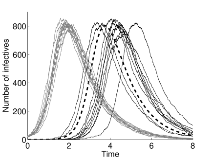
Figure 1: Examples of realizations of two randomized SIR models. The total number of infectives is plotted in node 1 ($I_{1}^{\Sigma}=I_{1}+I_{21}$) by thin grey lines and in node 2 ($I_{2}^{\Sigma}=I_{2}+I_{12}$) by thin black lines. Bold dashed lines indicates the hydrodynamic limit. ($N_{1}=N_{2}=2$k, ${\rm Ro}_{1}={\rm Ro}_{2}=4$, $\varepsilon=0.01,\tau=5$, $I_{0}/N_{1}=0.01$)

In the first set of numerical experiments the total population size varies from $N_{1}=N_{2}=N=400$ up to 10⁶. Number of realization $L$ was taken $10^{4}$ mainly but the number of realization is taken greater for small population $N=400$ and $2000$ and smaller for extremely high populations: 250k and 1000k. The current mean number of total infectives $\bar{I}_{1,2}^{\Sigma}(t)$ and standard deviation are computed. The results of the first set are shown in Figure 2. Observe that the mean value of the random process (thin lines) converges to the solution of correspondent deterministic problem (bold lines). But the convergence is much slower for node 2: for $N_{1}=10$k the mean trajectory practically coincides with the deterministic limit, on the other side the same effect in node 2 requires $N_{2}\sim 250$k.

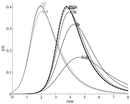
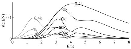
Figure 2: Evolution of the mean values for $I^{\Sigma}_{m}/N_{m}$ $m=1,2$ (left) and their standard deviations (right). Grey curves for node 1, black lines for node 2. Dashed lines indicate the hydrodynamic limit described by eqs. (4)–(7). The node population is indicated near the top of the correspondent curve.

The convergence rate is examined in Figure 3. One can see that for node 1 the convergence rate almost coincides with $O(N^{-1/2})$, as for node 2 the decay rate tends to $O(N^{-1/2})$ only for sufficiently large population: $N=10^{6}$. Thus for the secondary contaminated node the account of randomness is essential even if its population is large provided that the migration parameters $\varepsilon_{1,2}^{I,S}$ are small (0.01 in this case). Say, if $N_{2}=400$ the standard deviation exceeds the mean value up to the outbreak time.

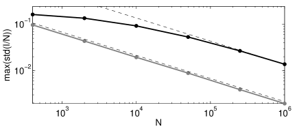
Figure 3: Maximal value of the standard deviation for processes $I_{1}/N_{1}$ and $I_{2}/N_{2}$ vs population $N=N_{1}=N_{2}$. Black curves for node 1, grey lines for node 2. The slope of dashed line corresponds to the decay law $N^{-1/2}$.

In the second set of numerical experiments we study dependence of mean number of infectives and their standard deviation from the initial number of infectives $I_{0}$ in node 1. It varies from $1$ to $100$ (the share $i_{0}=I_{0}/N_{1}$ varies from $10^{-4}$ to $10^{-2}$). The results are plotted in Figure 4.

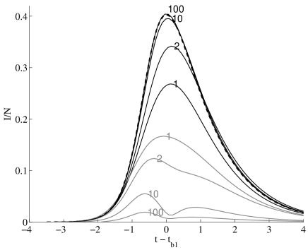
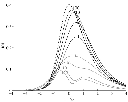
Figure 4: Left: Mean values for $I_{1}^{\Sigma}/N_{1}$ (black) and its standard deviation $\mathrm{std}{I_{1}^{\Sigma}/N_{1}}$ (grey) for different $I_{0}$. The initial number of infectives in node 1 is indicated near top of the corresponding curve. Dashed line indicates the deterministic limiting solution. Right: the same for $I_{2}^{\Sigma}/N_{2}$.

Because the outbreak time depends on initial number of infectives, the mean-field curves become essentially different. Therefore it is appropriate to shift the time so that the peak outbreak for different initial condition is at the same instant, say, $t=0$. Then all the curve are very close to each other and practically coincide with curve for the limiting solution introduces in [4, 5]. Observe that the smaller the number of initial infectives the greater is the standard deviation (std) and the larger is the difference between the mean curve for randomized process and the mean-field curve. Also observe that for node 1, the discrepancy of mean number of infectives from the hydrodynamic limit as well as the standard deviation monotonically decay with the growth of $I_{0}$. In node 2 the analogous discrepancy and the std slightly change when the number of initial infective varies from 10 to 100.

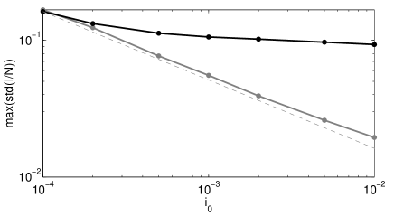
Figure 5: Maximal value of the standard deviation for $I_{1}/N_{1}$ and $I_{2}/N_{2}$ process vs population $I_{0}$ Grey curve is for node 1, black curve is for node 2. The dashed line has the slope corresponding to the decay law $N^{-1/2}$.

In the third set of numerical experiments we study dependence of the mean number of infectives on the coupling coefficient $\varepsilon$ (the same for all species). It was varied in the range $10^{-4},...,10^{-1}$. The results are plotted in Figures 6 and 7. Observe that $\varepsilon$ practically does not affect the standard deviation of total number of infectives in node 1. Discrepancy of the mean curve from the mean-field curve becomes noticeable only for small $\varepsilon$: $\varepsilon\lesssim 0.05$.

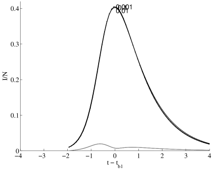
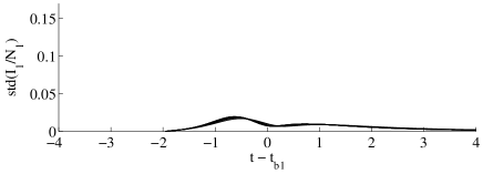
Figure 6: Mean values for $I_{1}^{\Sigma}/N_{1}$ (left) and its standard deviations $\mathrm{std}{I_{1}^{\Sigma}/N_{1}}$ (right) for different migration coefficient $\varepsilon$. Dashed lines indicate the mean-field limit. The initial number of infectives in node 1 is indicated near top of the corresponding curve.

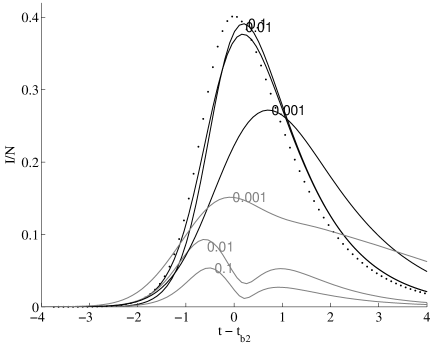
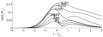
Figure 7: Mean values for $I_{2}^{\Sigma}/N_{2}$ (left) and its standard deviations $\mathrm{std}{I_{2}^{\Sigma}/N_{2}}$ (right) for different migration coefficient $\varepsilon$. Dashed lines indicate the mean-field limit. The initial number of infectives in node 1 is indicated near top of the corresponding curve.

As for the second node, the standard deviation grows monotonically with the decrease of the coupling. That indicates the importance to account for randomness of the epidemic process in the case of weak coupling (i.e. in the case of relatively slow migration fluxes).

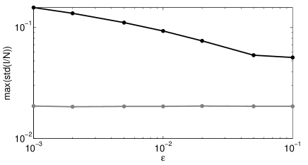
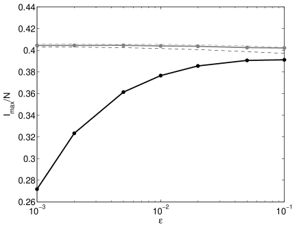
Figure 8: Left: Maximal value of the standard deviation for processes $I_{1}/N_{1}$ and $I_{2}/N_{2}$ vs population $N=N_{1}=N_{2}$. Grey curve is for node 1, black curve is for node 2. The dashed line has the slope corresponding to the decay law $N^{-1/2}$. Right: Outbreak value for $I_{1}/N_{1}$ and $I_{2}/N_{2}$ processes vs population $N=N_{1}=N_{2}$ Grey curve is for node 1, black curve is for node 2. The dashed line are for the mean-field values.

4 Two-stage semi-randomized model

The MC model for two coupled SIR centra can be readily generalized for an arbitrary network of $M$ mutually interacting SIR centers:

Process Rate

$$S_{n}\rightarrow S_{n}{-}1,I_{n}\rightarrow I_{n}{+}1$$

(26)

where $m,n=1,...,M,m\neq n$.

Generically, to study migration fluxes ($\gamma_{nm}^{S,I},\delta_{mn}^{S,I}>0$) between every pair of centers (although of different rates) we have to consider $2M$ host and $2M(M-1)$ guest species. The correspondent MC model will contain $4M^{2}$ fluxes. The total rate can be evaluated via $\nu_{\Sigma}=O(M^{2}N^{2})$. Therefore for a network containing significant number of highly populated centra (say, main cities in the UK), the time interval $\Delta t$ will have to be taken extremely small, and, hence, the GPU time for a single realization will be too long to get the necessary statistics. Thus the MC should be simplified for numerical modelling.

4.1 The small initial contagion (SIC) approximation

The SIC approximation is based on the assumptions which look relevant for a network of highly populated centers:

• Population in every center is high: $N_{n}\gg 1$.

• Migration fluxes between the centers are small: $\varepsilon_{nm}^{S,I}\ll 1$.

• Initial number of infectives in the first contaminated center (say, $n=1$), is small: $I_{0}\ll N_{1}$.

• Reproduction number exceeds unity and is not close to it in all the nodes: $\mathrm{Ro}_{n}:=\beta_{n}N_{n}/\alpha_{n}>1+r$ where $r=O(1),r>0$.

In these assumptions, the outbreak process in every center can be split into the following main stages:

1. Contaminating stage: number of infectives is small $I_{n}\ll N_{n},S_{n}\approx N_{n}$ and the fluxes of infectives caused by migration are essential for the outbreak process (except the first node).

2. Developed outbreak: $I_{n}\gg 1$, when the contribution of migration fluxes is negligible, (also the mean-field description for every individual realization looks adequately).

3. Recovering stage: the node is not affected by infective immigrants and slightly affects contamination of other nodes.

From these assumptions follows that the outbreak dynamics in the first node can be considered independently, and can be described by the following MC

Process Rate

$$S_{1}\rightarrow S_{1}{-}1,I_{1}\rightarrow I_{1}{+}1$$

(27)

with the initial condition $I_{1}(0)=I_{0}$, $S_{1}=N_{1}-I_{0}$ studied in [7, 3]. At the contamination stage we have $S_{1}\approx N_{1}$ and the MC can be further simplified

Process Rate

$$I_{1}\rightarrow I_{1}{+}1$$

(28)

Epidemic dynamics in node 2 at the contamination stage ($S_{2}\approx N_{2}$) can be described by analogous MC with additional flux $\nu(t)$ of infectives migrated from node 1:

Process Rate

$$I_{2}\rightarrow I_{2}{+}1$$

   (29)

with $I_{2}(0)=0$ where

$$\nu(t)=(\beta_{2}N_{2})I_{12}+\delta_{12}^{I}I_{21}.$$ (30)

At the contamination stage processes $I_{12}(t)$ and $I_{21}(t)$ are practically independent of process $I_{2}(t)$. Thus we have to consider MC (29) with a random flux $\nu(t)$ which statistics will be specified later.

4.2 Calculation of moments

First we consider a single realization of the flux $\nu(t)$ and treat it as a deterministic function. Later we will use averaging on $\nu(t)$ to calculate moments of distribution for $I_{2}(t)$.

4.2.1 Calculation of PGF for a single realization $G(z,t)$.

Let $P_{k}(t)=\mathbb{P}(I_{2}(t)=k)$ be the probability of $k$ infectives $I_{2}$ at instant $t$. Initial condition is

$$P_{0}(0)=1,\qquad P_{k>0}(0)=0.$$ (31)

Kolmogorov’s equations for MC (29) are

$$\textstyle{\frac{\mathrm{d}}{\mathrm{d}t}}P_{k}=\beta_{2}^{\prime}(\left\lceil k-1\right\rceil_{0}^{N_{2}})P_{k-1}-\beta_{2}^{\prime}kP_{k}+\displaystyle\alpha_{2}(\left\lceil k+1\right\rceil_{0}^{N_{2}})P_{k+1}-\alpha_{2}kP_{k}+\nu P_{k-1}-\nu P_{k}.$$ (32)

Here $\beta_{2}^{\prime}=\beta_{2}N_{2}$. For the PGF $G(z,t)$ tending $N_{2}\rightarrow\infty$ (with $\beta_{2}\rightarrow 0$, $\beta_{2}^{\prime}=const$) we obtain the following PDE

$$G_{t}=(z-1)\left[\left(\beta_{2}^{\prime}z-\alpha_{2}\right)G_{z}+\nu(t)G\right]$$ (33)

with the initial condition $G(z,0)=1$. Its solution can be written in the integral form

$$G(z,t)=\exp\!\Big{\{}\!-\int_{0}^{t}\frac{\lambda_{2}(z{-}1)\,\nu\left(t^{\prime}\right)\,\mathrm{d}t^{\prime}}{\beta_{2}^{\prime}(z{-}1)-(\beta_{2}^{\prime}z{-}\alpha_{2})\,e^{\lambda_{2}(t^{\prime}{-}t)}}\Big{\}}$$ (34)

where $\lambda_{2}=\beta_{2}^{\prime}-\alpha_{2}$ is the initial growth rate of infectives in the deterministic SIR model in the limit $I_{0}/N\rightarrow 0$ (limiting solution introduced in [4, 5]).

4.2.2 Calculation of first moment $\mathbb{E}\left[I_{2}\left(t\right)\right]$.

The first conditional moment $\mu_{1}(t\,|\,\nu)=\mathbb{E}(I_{2}(t)\,|\,\nu)$ for fixed $\nu(t)$ is

$$\mu_{1}(t\,|\,\nu)=G_{z}(1,t)=\int_{0}^{t}\nu\left(t^{\prime}\right)e^{\lambda_{2}(t-t^{\prime})}\mathrm{d}t^{\prime}$$ (35)

Averaging over all realizations for $\nu(t)$ (with a time varying PDF $f_{\nu}(t)$): $\mu_{1}(t)=\mathbb{E}\mu_{1}(t\,|\,\nu)$

$$\mu_{1}(t)=\int\Big{[}\int_{0}^{t}f_{\nu}(t^{\prime})\nu\left(t^{\prime}\right)e^{\lambda_{2}(t-t^{\prime})}\mathrm{d}t^{\prime}\Big{]}\mathrm{d}\nu=\int_{0}^{t}\bar{\nu}\left(t^{\prime}\right)e^{\lambda_{2}(t-t^{\prime})}\mathrm{d}t^{\prime}$$ (36)

where $\bar{\nu}(t)=\mathbb{E}\nu(t)$. Thus the average number of infectives in node 2 in the contamination stage relates with the flux $\nu(t)$ via the convolution

$$\mathbb{E}\left[I_{2}\left(t\right)\right]\equiv\mu_{1}\left(t\right)=\bar{\nu}\left(t\right)\ast e^{\lambda_{2}t}.$$ (37)

4.2.3 Calculation of second moment $\mathrm{var}[I_{2}(t)]$.

To calculate it we apply the Law of Total Variation  (e.g. [2]):

$$\mathrm{var}\left[I_{2}(t)\right]=\mathbb{E}\left[\mathrm{var}(I_{2}(t)\,|\,\nu)\right]+\mathrm{var}\left[\mathbb{E}(I_{2}(t)\,|\,\nu)\right].$$ (38)

1. The first addend in (38) can be found through the PGF $G(z,t)$:

$$\begin{array}[]{l}\mathrm{var}(I_{2}(t)\,|\,\nu)=\displaystyle G_{zz}(1,t)+\mu_{1}(t\,|\,\nu)-\mu_{1}^{2}(t\,|\,\nu)\\ \displaystyle=\frac{2\beta_{2}^{\prime}}{\lambda_{2}}\int_{0}^{t}\nu(t^{\prime})\left[e^{2\lambda_{2}(t-t^{\prime})}-e^{\lambda_{2}(t-t^{\prime})}\right]\mathrm{d}t^{\prime}+\mu_{1}(t\,|\,\nu).\end{array}$$

After the averaging through $\nu$ we obtain

$$\mathbb{E}\left[\mathrm{var}(I_{2}(t)\,|\,\nu)\right]=\displaystyle\mu_{1}(t)+\frac{2\beta_{2}^{\prime}}{\lambda_{2}}\int_{0}^{t}\bar{\nu}(t^{\prime})\left[e^{2\lambda_{2}(t-t^{\prime})}-e^{\lambda_{2}(t-t^{\prime})}\right]\mathrm{d}t^{\prime}.$$

Thus a first addend in (38) can written as a sum of two convolutions

$$\mathbb{E}\left[\mathrm{var}(I_{2}(t)\,|\,\nu)\right]=\frac{2\beta_{2}^{\prime}}{\lambda_{2}}\bar{\nu}(t)\ast e^{2\lambda_{2}t}+(1-\frac{2\beta_{2}^{\prime}}{\lambda_{2}})\bar{\nu}(t)\ast e^{\lambda_{2}t}$$ (39)

where $\bar{\nu}(t)=\beta_{2}^{\prime}\bar{I}_{12}(t)+\delta_{12}^{I}\bar{I}_{21}(t)$.

2. To calculate the second addend in (38), we temporary add $\mu_{1}^{2}$ to it. Now it can be expressed via the covariance of flux $\nu(t)$:

$$\begin{array}[]{l}\displaystyle\mathrm{var}\left[\mathbb{E}(I_{2}(t)\,|\,\nu)\right]+\mu_{1}^{2}(t)=\mathbb{E}\left(\int_{0}^{t}\nu\left(t^{\prime}\right)e^{\lambda_{2}(t-t^{\prime})}\mathrm{d}t^{\prime}\right)^{2}\\[6.0pt] \displaystyle=\int_{0}^{t}\int_{0}^{t}\mathbb{E}\left[\nu\left(t^{\prime}\right)\nu\left(t^{\prime\prime}\right)\right]e^{\lambda_{2}(t-t^{\prime})}\mathrm{d}t^{\prime}e^{\lambda_{2}(t-t^{\prime\prime})}\mathrm{d}t^{\prime\prime}.\end{array}$$ (40)

The function in the integrand can be represented as a sum

$$\mathbb{E}\left[\nu\left(t^{\prime}\right)\nu\left(t^{\prime\prime}\right)\right]=\mathrm{cov}\left[\nu\left(t^{\prime}\right),\nu\left(t^{\prime\prime}\right)\right]+\bar{\nu}(t^{\prime})\bar{\nu}(t^{\prime\prime}).$$ (41)

Integration of the second addend in (41) gives just the temporary added term

$$\int_{0}^{t}\int_{0}^{t}\bar{\nu}(t^{\prime})\bar{\nu}(t^{\prime\prime})e^{\lambda_{2}(t-t^{\prime})}\mathrm{d}t^{\prime}e^{\lambda_{2}(t-t^{\prime\prime})}\mathrm{d}t^{\prime\prime}=\mu_{1}^{2}(t).$$

Thus the second addend in (38) can be written through the following integral

$$\mathrm{var}\left[\mathbb{E}\big{(}I_{2}(t)\;|\;\nu\big{)}\right]=\int_{0}^{t}\int_{0}^{t}\mathrm{cov}\left[\nu\left(t^{\prime}\right),\nu\left(t^{\prime\prime}\right)\right]e^{\lambda_{2}(t-t^{\prime})}\mathrm{d}t^{\prime}e^{\lambda_{2}(t-t^{\prime\prime})}\mathrm{d}t^{\prime\prime}.$$ (42)

in which we have to calculate the covariance of flux $\nu(t)$.

If flux $\nu(t)$ is a random process controlled by a MC, calculation of its covariance is a complicated task, and consideration of this needs a separate work. Remind that the flux is a linear combination of two MC processes (30): $\nu(t)=\beta_{2}^{\prime}I_{12}(t)+\delta_{12}^{I}I_{21}(t)$. Here we approximate $I_{12}(t)$ and $I_{21}(t)$ by two mutually independent Poisson processes with variable rates $\frac{\mathrm{d}}{\mathrm{d}t}\bar{I}_{12}(t)$ and $\frac{\mathrm{d}}{\mathrm{d}t}\bar{I}_{21}(t)$, respectively, where $\bar{I}_{12}(t)$ and $\bar{I}_{21}(t)$ are calculated below. In this approximation, using the independence of increments of the inhomogeneous Poisson flow (e.g. [11]) we can write

$$\mathrm{cov}\left[I_{12}\left(t^{\prime}\right),I_{12}\left(t^{\prime\prime}\right)\right] \approx \bar{I}_{12}(\min\left\{t^{\prime},t^{\prime\prime}\right\}),$$

$$\mathrm{cov}\left[I_{21}\left(t^{\prime}\right),I_{21}\left(t^{\prime\prime}\right)\right] \approx \bar{I}_{21}(\min\left\{t^{\prime},t^{\prime\prime}\right\}),$$

$$\mathrm{cov}\left[I_{12}\left(t^{\prime}\right),I_{21}\left(t^{\prime\prime}\right)\right] \approx 0.$$

We justify this approximation numerically below. Thus, for the covariance of the flux we have

$$\mathrm{cov}\left[\nu\left(t^{\prime}\right),\nu\left(t^{\prime\prime}\right)\right]=\varpi(\min\left\{t^{\prime},t^{\prime\prime}\right\}),\quad\varpi(t)\equiv\left(\beta_{2}^{\prime}\right)^{2}\bar{I}_{12}(t)+\left(\delta_{12}^{I}\right)^{2}\bar{I}_{21}(t).$$ (43)

Equation (43) holds true because the second central moment of the Poisson process coincides with the first moment. In this approximation, it is sufficient to compute the first moment of flux $\nu(t)$ in order to compute the second moment for $I_{2}$.

With the account for (43), we split integral (42) into two parts:

$$\mathrm{var}\left[\mathbb{E}\big{(}I_{2}(t)\;|\;\nu\big{)}\right] \approx J_{1}+J_{2}$$

$$J_{1} = \int_{0}^{t}\int_{0}^{t^{\prime}}\varpi(t^{\prime\prime})e^{\lambda_{2}(t-t^{\prime\prime})}\mathrm{d}t^{\prime\prime}e^{\lambda_{2}(t-t^{\prime})}\mathrm{d}t^{\prime}$$

$$J_{2} = \int_{0}^{t}\int_{t^{\prime}}^{t}\varpi(t^{\prime})e^{\lambda_{2}(t-t^{\prime\prime})}\mathrm{d}t^{\prime\prime}e^{\lambda_{2}(t-t^{\prime})}\mathrm{d}t^{\prime}.$$

Integrating $J_{1}$ by parts and $J_{2}$ directly we obtain that they both give the same answer

$$J_{1}=J_{2}=\frac{1}{\lambda_{2}}\varpi(t)\ast e^{2\lambda_{2}t}-\frac{1}{\lambda_{2}}\varpi(t)\ast e^{\lambda_{2}t}.$$

Finally combining the above results we have

$$\begin{array}[]{l}\mathrm{var}(I_{2})=\displaystyle\frac{4\left(\beta_{2}^{\prime}\right)^{2}}{\lambda_{2}}\bar{I}_{12}\ast e^{2\lambda_{2}t}+\Big{[}\frac{2\beta_{2}^{\prime}\delta_{12}^{I}}{\lambda_{2}}+\frac{2\left(\delta_{12}^{I}\right)^{2}}{\lambda_{2}}\Big{]}\bar{I}_{21}\ast e^{2\lambda_{2}t}\\[8.39996pt] \displaystyle\;{}-\Big{[}\frac{4\left(\beta_{2}^{\prime}\right)^{2}}{\lambda_{2}}-\beta_{2}^{\prime}\Big{]}\bar{I}_{12}\ast e^{\lambda_{2}t}-\Big{[}\frac{2\beta_{2}^{\prime}\delta_{12}^{I}}{\lambda_{2}}+\frac{2\left(\delta_{12}^{I}\right)^{2}}{\lambda_{2}}-\delta_{12}^{I}\Big{]}\bar{I}_{21}\ast e^{\lambda_{2}t}.\end{array}$$ (44)

4.2.4 Computation of the average flux $\bar{\nu}(t)$.

It is natural to split the total flux into two parts $\nu(t)=\beta_{2}^{\prime}I_{12}+\delta_{12}^{I}I_{21}=\nu_{12}(t)+\nu_{21}(t)$. Flux process $\nu_{12}(t)$ described by the MC

Process Rate

$$I_{12}\rightarrow I_{12}{+}1$$

(45)

(with $I_{12}(0)=0$) coincides with that described by (29) if we set $\beta_{2}^{\prime}\leftarrow 0$, $\nu(t)\leftarrow\gamma_{12}^{I}I_{1}$, $\alpha_{2}\leftarrow\left(\delta_{21}^{I}+\alpha_{2}\right)$. Then we can immediately write down a solution for the PGF

$$G(z,t)=\exp\!\big{\{}\gamma_{12}^{I}\left(z{-}1\right)\!\!\!\int_{0}^{t}I_{1}\left(t^{\prime}\right)e^{-\left(\delta_{21}^{I}+\alpha_{2}\right)(t^{\prime}-t)}\mathrm{d}t^{\prime}\!\big{\}}$$

and the first moment

$$\bar{I}_{12}=\gamma_{12}^{I}\int_{0}^{t}\bar{I}_{1}\left(t^{\prime}\right)e^{-(\delta_{21}^{I}+\alpha_{2})(t-t^{\prime})}\mathrm{d}t^{\prime}.$$ (46)

Flux process $\nu_{21}$ is more complicated and can be described by the following MC

Process Rate

$$S_{21}\rightarrow S_{21}+1$$

(47)

with the initial conditions $S_{21}(0)=\varepsilon_{21}^{S}N_{2}$, $I_{21}(0)=0$. If we split the third event into two independent events $I_{21}\rightarrow I_{21}+1$ and $S_{21}\rightarrow S_{21}-1$ with the same rate, we can split MC (47) into two MCs. The first MC describes migration of host susceptives from node 2 to node 1 and their possible removal due to contamination:

Process Rate

$$S_{21}\rightarrow S_{21}+1$$

(48)

It is independent of the second MC with the rates

Process Rate

$$I_{21}\rightarrow I_{21}+1$$

(49)

which describes migration of susceptibles to a neighbor node, their contamination there and return to the host node as infected species.

First, we study the first MC: (48). In accordance with  (19) it has the binomial initial distribution:

$$P_{k}(0)=\binom{N_{2}}{k}\left(\varepsilon_{21}^{S}\right)^{k}\left(1-\varepsilon_{21}^{S}\right)^{N_{2}-k}.$$ (50)

The probabilities $P_{k}(t)=\mathbb{P}(S_{21}(t)=k)$ of $k$ guest susceptibles $S_{21}$ at instant $t$ satisfy Kolmogorov’s equations for MC (29)

$$\textstyle{\frac{\mathrm{d}}{\mathrm{d}t}}P_{k}=\nu\left(P_{k-1}-P_{k}\right)+\alpha\left[(\left\lceil k+1\right\rceil_{0}^{N_{2}})P_{k+1}-kP_{k}\right].$$ (51)

where $\nu=\gamma_{21}^{S}N_{2}$, $\alpha=\left(\delta_{12}^{S}+\beta_{1}I_{1}\right)$. System (51) implies the following PDE for MGF $G(z,t)=\sum_{k=0}^{\infty}z^{k}P_{k}(t)$

$$G_{t}=(z-1)\left[-\alpha(t)G_{z}+\nu G\right].$$ (52)

The initial condition is

$$G(z,0)=\sum\limits_{k=0}^{N}z^{k}\binom{N}{k}\varepsilon^{k}(1-\varepsilon)^{N-k}=(1-\varepsilon+\varepsilon z)^{N}.$$ (53)

The initial value problem (52)–(53) admits the explicit solution

$$G(z,t)=\left[1+\varepsilon(z-1)\phi(t)\right]^{N}\exp\left\{\nu(z-1)\phi(t)\int_{0}^{t}\frac{\mathrm{d}t^{\prime}}{\phi(t^{\prime})}\right\}.$$ (54)

where $\phi(t)=\exp\left\{-\int_{0}^{t}\alpha(t^{\prime})\mathrm{d}t^{\prime}\right\}$. From here we have

$$\mathbb{E}S_{21}(t)=G_{z}(1,t)=N_{2}\left[\varepsilon_{21}^{S}+\gamma_{21}^{S}\int_{0}^{t}\mathrm{d}t^{\prime}/\phi(t^{\prime})\right]\phi(t).$$ (55)

Now for process (49) in analogy with processes (29) and (45) we can immediately write

$$\bar{I}_{21}=\beta_{1}\int_{0}^{t}e^{-\left(\delta_{12}^{I}+\alpha_{2}\right)(t-t^{\prime})}\mathbb{E}\left[I_{1}\left(t^{\prime}\right)S_{21}(t^{\prime})\right]\mathrm{d}t^{\prime}.$$ (56)

Neglecting the mutual dependence of processes $S_{21}(t)$ and $I_{1}(t)$ we approximate

$$\mathbb{E}\left[S_{21}(t)I_{1}(t)\right]\approx\mathbb{E}S_{21}(t)\bar{I}_{1}(t).$$ (57)

Below we show numerically that it is satisfactory approximation for our applications.

4.3 The second stage

Remind that equations (36), (42), (43), (44), (46), (56), (57) are valid at the contamination stage only ($S_{2}\approx N_{2}$). They allow us to calculate the first and second moments for the number of infectives without modelling the random process directly. To evaluate the moments at the developed outbreak we use the same approach as in [3]: by approximating the outbreak via the mean field solution for a single SIR node with random initial conditions.

For this aim we define the intermediate time $t_{\ast}$ such that the number of infective is large enough to use the mean field solution but the number of infective still slightly deviate from $N_{2}$: $\hat{I}_{2}(t_{\ast})\gg 1$ and $N_{2}-\hat{S}_{2}\ll N_{2}$.

Then we generate $L$ times a random number $X$ lognormally distributed (to guarantee the positiveness) with mean $\bar{I}_{2}(t_{\ast})$ and variance $\mathrm{var}(I_{2}(t_{\ast}))$ and integrate the classical SIR equations: $\frac{\mathrm{d}}{\mathrm{d}t}\hat{S}_{2}=-\beta_{2}\hat{S}_{2}\hat{I}_{2}$, $\frac{\mathrm{d}}{\mathrm{d}t}\hat{I}_{2}=(\beta_{2}\hat{S}_{2}-\alpha_{2})\hat{I}_{2}$ with initial condition $\hat{I}_{2}(t_{\ast})=X$,

$$\hat{S}_{2}(t_{\ast})=-W_{-1}\left[-\beta_{2}^{\prime}N_{2}\exp\left\{\beta_{2}^{\prime}(X-N_{2})\right\}\right]/\beta_{2}^{\prime}$$

where $W_{k}[\cdot]$ is the $k$th branch of the Lambert function [12].

Let us emphasize that in the classical SIR model, the numbers of susceptives and infectives are related as $I=N-S+\ln\left[S/(N-I_{0})\right]/\beta^{\prime}$ where $\beta^{\prime}=\beta N$ (cf. [7]). Resolving this relation with respect to $S$ we can write

$$S=-W_{k}\left[-\beta^{\prime}(N-I_{0})\exp\left\{\beta^{\prime}(I-N)\right\}\right]/\beta^{\prime}$$

where $k=-1$ for the growing part and $k=0$ for the decaying part of the outbreak. If the outbreak is triggered by a infinitesimal number of infectives we can set $S=-W_{k}\left[-\beta^{\prime}N\exp\left\{\beta^{\prime}(I-N)\right\}\right]/\beta^{\prime}$.

Also note that it is natural to approximate the solution to a standard SIR model by the limiting solution ($I_{0}/N\rightarrow 0$) introduced in [4]. The limiting solution is independent of the initial condition, therefore it is not necessity to integrate the ODEs $L$ times but only once.

Thus the proposed two-stage model of a coupled randomized epidemic centers allows us to calculate its first moments much faster than the direct simulation summarized in Table 1.

4.4 Comparison with numerical simulation

To show the accuracy of the proposed model we compare the solution obtained by different approaches. Again the basic model of Section 3 is used: $N_{1}=N_{2}=10$k, $\beta_{1,2}^{\prime}=4$, $\alpha_{1,2}=1$, $\varepsilon_{1,2}^{S,I}=0.01$, $\tau_{1,2}^{S,I}=5$, $I_{0}/N_{1}=0.01$but also model with the smaller population $N_{1}=N_{2}=2$k. We compare (i) the full randomized model described in Table 1 which we regard as a benchmark; (ii) the SIC approximate randomized model where only flux of infectives from node 1 to node 2 is accounted, it is described in Table 2; (iii) the two-stage semi-randomized model proposed in this section above.

In the two-stage model we take time $t_{\ast}=2.0$ for transition from a contamination randomized stage to the mean-field stage with random initial condition. The expected number of infectives in node 2 at time $t=2.0$ is $100$ which is large enough and at the same time much smaller than the node population. We take $L=10^{4}$ for number of realization in the second stage to evaluate the moments.

In the SIC approximation the randomized model presented in Table 2 comprises four consequently independent MCs. Processes 1 and 2 represent independent outbreak in node 1 (27). Processes 3 and 4 represent migration of its infectives to node 2 (45). Processes 5 and 6 represent migration of host susceptives from node 2 to node 1 and their possible removal due to contamination; they are analogous to MC (48) with $N_{2}$ substituted by $S_{2}$ to be valid for all the stages. Analogously processes 7 and 8 represent contamination of $S_{21}$ in the first node and migration of appeared infectives $I_{21}$ to their host node (49). Finally processes 9–10 represent the outbreak in node 2 ; they are analogous to MC with an additional flux (29) with the accurate account of the number of succeptives $S_{2}$ at all the stages.

Table 2: Markov’s chain for two coupled SIR nodes in the SIC approximation

#	Process	Rate
1	$\begin{array}[]{l}S_{1}\rightarrow S_{1}{-}1\\ I_{1}\rightarrow I_{1}{+}1\end{array}$	$\beta_{1}I_{1}S_{1}$
2	$I_{1}\rightarrow I_{1}{-}1$	$\alpha_{1}I_{1}$
3	$I_{12}\rightarrow I_{12}{+}1$	$\gamma_{12}^{I}I_{1}$
4	$I_{12}\rightarrow I_{12}-1$	$\delta_{21}^{I}I_{12}$
5	$S_{21}\rightarrow S_{21}{+}1$	$\gamma_{21}^{S}S_{2}$
6	$S_{21}\rightarrow S_{21}{-}1$	$\left(\delta_{12}^{S}+\beta_{1}I_{1}\right)S_{21}$
7	$I_{21}\rightarrow I_{21}{+}1$	$\beta_{1}I_{1}S_{21}$
8	$I_{21}\rightarrow I_{21}{-}1$	$\alpha_{1}I_{21}$
9	$\begin{array}[]{l}S_{2}\rightarrow S_{2}{-}1\\ I_{2}\rightarrow I_{2}{+}1\end{array}$	$\beta_{2}(I_{2}+I_{12})S_{2}+\delta_{12}^{I}I_{21}$
10	$I_{2}\rightarrow I_{2}{-}1$	$\alpha_{2}I_{2}$

The results of computation are presented in Figures 9 and 10. Here the bold lines indicate the full randomized model, the thin solid lines indicate the SIC approximated model, the line with dots indicate the two-stage semi-randomized model. Also the mean-field solution is presented as well and indicated by dashed lines.

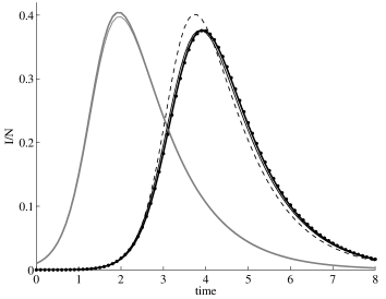
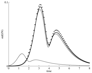
Figure 9: Comparison of different approximation for the mean value of infectives (left) and its standard deviation (right) for the populations $N_{1}=N_{2}=10$k. Bold line – full randomized model (Table 1), thin line – approximate randomized model (Table 2), line with dots – the proposed two-stage semi-randomized model, dashed line – the mean field solution.

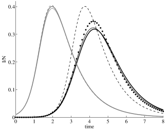
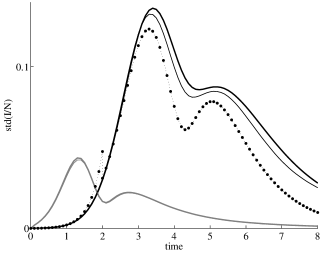
Figure 10: The same as in Figure 9 but for $N_{1}=N_{2}=2$k.

Evidently, the proposed two-stage semi-randomized model gives a quite satisfactory approximation for the first two moments of total number of infectives in node 2 if the population is $10$k but only qualitative similarity for the smaller population. This justifies the used simplifications for rather moderate populated sites, but for the sites with population 2k and smaller a more sophisticated models should be developed. This can be a material of the consequent works.

5 Discussion

The randomized network SIR model coupled by randomized migration fluxes is described in terms of a Markov chain (MC). In the absence of infectives the pure migration model give reasonable modelling of migration of individuals is described as a simple MC: being disturbed the system returns to a dynamic equilibrium exponentially fast that resembles a diffusion process in physics.

In the mean-field (hydrodynamic) limit the MC converges to a non-standard network SIR model: the host and guest species are treated separately in the corresponding ODEs (4)–(7).

Note that traditionally the coupling with other nodes is described by adding some transport terms (cf. [7, 13])

$$\begin{array}[]{rcl}{\frac{\mathrm{d}}{\mathrm{d}t}}S_{n}&=&-\beta_{n}S_{n}I_{n}+\chi_{mn}^{S}S_{m}\\ {\frac{\mathrm{d}}{\mathrm{d}t}}I_{n}&=&\beta_{n}S_{n}I_{n}-\alpha_{n}I_{n}+\chi_{mn}^{I}I_{m}\end{array}$$

Simple analysis shows that pure migration in the such equation results in exponentially growing solutions [8]. This instability is ignored as it can be hidden in the background of the outbreak and not be observable in certain epidemic model scenarios.

The model proposed in [14, 15]

$$\begin{array}[]{rcl}{\frac{\mathrm{d}}{\mathrm{d}t}}S_{n}&=&-\beta_{n}S_{n}I_{n}+\chi_{mn}^{S}S_{m}-\chi_{nm}^{S}S_{n}\\ {\frac{\mathrm{d}}{\mathrm{d}t}}I_{n}&=&\beta_{n}S_{n}I_{n}-\alpha_{n}I_{n}+\chi_{mn}^{I}I_{m}-\chi_{nm}^{I}I_{n}\end{array}$$

gives more stable pure migration but the simple analysis shows that in this model we obtain the fully mixed population in all the nodes [8] ($\varepsilon=0.5$ in our terms). Thus the dynamics of this model seems to be more realistic but nevertheless does not satisfy an intuitive interpretation of the equilibrium of the migration process.

The both above models are characterized by only one parameter describing migration of a given species. This makes impossible to tune the model to obtain the realistic migration in the absence of the outbreak.

In our earlier work [5] a migration model is introduced without splitting species into host and guest with two migration parameters: $\varepsilon$ and $\tau$ describing migration process of a given species. But model proposed in [5] also does not give a completely satisfactory solution for pure migration in the case of different migration times: $\tau_{12}^{S}$ and $\tau_{21}^{S}$ as shown in [8].

Note that for some combination of the network parameters (epidemic and migration) effect of the more correct accounting of migration can be very small but it can become essential when parameters of the model vary.

It is interesting to compare three different techniques for the model under consideration: a MC describing the number of individuals from all categories in both centers, its hydrodynamical limit in the form of a system of dynamic equations and a simple description of contamination stage at the node 2 as an isolated center with an inflow of infectives neglecting the backward migration. We developed an approach when the random evolution on the contamination stage either in its full or simplified form is coupled with the dynamical description on the stage of saturation. This makes the problem computationally feasible. Our intention is to apply this technique to a network of interacting population centers in the next paper. Note that the direct simulation of the network is far too expensive in terms of computational time compared with the integration of systems of dynamical equations. The computational time may be considerably reduced if the simulation is required during a relatively short contamination periods only.

The spatial dynamics of multi-species epidemic models is widely discussed in the literature (see [16, 17, 18, 19, 20, 21, 22, 23, 24] and the reference therein). For a purely deterministic model the account of different dynamics of host and guest species on the epidemic speed was studied in [8]. The simplifying assumptions make the analysis tractable by may not adequately reflect reality. It seems that a network of stochasticly interacting centres of the type discussed above may provide more realistic but still tractable setting.

In the next paper we intend to derive the traveling wave characteristic equation (cf. [4],[5],[8]) and explore analytically an numerically the dependence of the mean epidemic speed and its standard deviation on the network parameters.

Appendix A Sketch of the proof to Proposition 1.

First, the mean values of the Markov chain (MC) converges to the solution of initial value problem (4)–(9) by the LLN. Phenomenological sketch is given Section 1, and the rigorous proof is analogous to that presented in [25, 26].

We also have to establish the convergence in probability. For definiteness consider $I_{2}(t)$ and apply Chebyshev’s inequality for any $\epsilon>0$

$$\mathbb{P}\Big{(}\Big{|}\frac{I_{2}(t)}{\Lambda}-{\hat{I}}_{2}(t)\Big{|}>\epsilon\Big{)}\leq\frac{\mathrm{var}\left[I_{2}(t)\right]}{\Lambda^{2}\epsilon^{2}}.$$

Recall that $\Lambda$ is the population scaling parameter (see Section 1). So, it is enough to check that

$$\mathrm{var}\left[I_{2}(t)\right]=O(\Lambda),\qquad\Lambda\rightarrow\infty.$$ (58)

It is demonstrated numerically in Section 3 (see Figure 3). Actually we see that the normalized standard deviation decays as $N^{-1/2}$, or equivalently, the non-normalized standard deviation grows as $N^{1/2}$ (i.e., as $\Lambda^{1/2}$), that implies (58).

The rigorous argument runs as follows. Consider the processes in Table 1 which cause the change in number of infectives in node 2 and outline the fluxes of infectives. These processes are

$$\begin{array}[]{ccc}\hline\cr\hline\cr\mbox{\#}&\mbox{Event}&\mbox{Rate}\rule[-6.02289pt]{0.0pt}{18.0672pt}\\ \hline\cr\hline\cr\mbox{9,16}&I_{2}\rightarrow I_{2}+1&\beta_{2}I_{2}S_{2}+\underline{\beta_{2}I_{12}S_{2}+\delta_{12}^{I}I_{21}}\rule[-6.02289pt]{0.0pt}{18.0672pt}\\ \hline\cr\mbox{11,14}&I_{2}\rightarrow I_{2}-1&\alpha_{1}I_{2}+\underline{\gamma_{21}^{I}I_{2}}\rule[-6.02289pt]{0.0pt}{18.0672pt}\\ \hline\cr\hline\cr\end{array}$$ (59)

Here the flux terms are underlined, the remaining terms describe the MC based stochastic SIR model [7, 3]. So the real flux can be defined as

$$\nu(t)=\beta_{2}I_{12}S_{2}+\delta_{12}^{I}I_{21}-\gamma_{21}^{I}I_{2}.$$

We construct the process $\tilde{I}_{2}$

$$\begin{array}[]{cc}\hline\cr\hline\cr\mbox{Event}&\mbox{Rate}\rule[-6.0pt]{0.0pt}{18.0pt}\\ \hline\cr\hline\cr\tilde{I}_{2}\rightarrow\tilde{I}_{2}+1&\beta_{2}^{\prime}\tilde{I}_{2}+\tilde{\nu}\rule[-6.0pt]{0.0pt}{18.0pt}\\ \hline\cr\tilde{I}_{2}\rightarrow\tilde{I}_{2}-1&\alpha_{1}\tilde{I}_{2}\rule[-6.0pt]{0.0pt}{18.0pt}\\ \hline\cr\hline\cr\end{array}$$ (60)

with the majorized constant flux

$$\tilde{\nu}=\beta_{2}^{\prime}N_{1}+\delta_{12}^{I}N_{2}\geq\nu(t).$$

Remind that $\beta_{2}^{\prime}=\beta_{2}N_{2}$ is a constant when $\Lambda\rightarrow\infty$.

For this process we have a randomized SI model (considered in [3]) with the constant Poisson flux $\tilde{\nu}$. This problem is solved in Section 4 and it is shown that its variance grows as $O(\Lambda)$.

Next, we establish the second order stochastic domination (see [27] for details) of process $I_{2}(t)$ by $\tilde{I}_{2}(t)$. In fact the following inequality holds for all $x,t\geq 0$ (cf. [27])

$$\int_{0}^{x}\;\mathbb{P}\big{(}I_{2}(t)\geq u\big{)}\mathrm{d}u\leq\int_{0}^{x}\;\mathbb{P}\big{(}{\tilde{I}}_{2}(t)\geq u\big{)}\mathrm{d}u.$$

The second order stochastic domination means that for any convex function $\Psi(.)$ we have the inequality for all $t\geq 0$

$$\mathbb{E}[\Psi(I_{2}(t))]\leq\mathbb{E}[\Psi({\tilde{I}}_{2}(t))],$$

${\tilde{I}}_{2}(t)$ is the number of susceptible in the tractable model described by (60). In our case $\Psi(X)=(X-\mathbb{E}X)^{2}$. This implies the inequality $\mathrm{var}\left[I_{2}(t)\right]\leq\mathrm{var}\left[\tilde{I}_{2}(t)\right]$. $\Box$

References

• [1]
• [2] S.M.Β Ross, First Course of Probability, NJ: Prentice Hall, 2008
• [3] I.Β Sazonov, M.Β Kelbert, M.Β B. Gravenor, A two-stage model for the sir outbreak: Accounting for the discrete and stochastic nature of the epidemic at the initial contamination stage, Mathematical Biosciences 234 (2011) 108–117.
• [4] I.Β Sazonov, M.Β Kelbert, M.Β B. Gravenor, The speed of epidemic waves in a one-dimensional lattice of SIR models, Mathematical Modelling of Natural Phenomena 3Β (4) (2008) 28–47.
• [5] I.Β Sazonov, M.Β Kelbert, M.Β B. Gravenor, Travelling waves in a network of sir epidemic nodes with an approximation of weak coupling, Mathematical Medicine and Biology 28Β (2) (2011) 165–183.
• [6] A.N.Β Nayfeh, Introduction to Perturbation Technique, N.Y.: J. Wiley $\&$ Sons, 1973.
• [7] D.Β Daley, J.Β Gani, Epidemic Modeling, Cambridge University Press, Cambridge, 1999.
• [8] I.Β Sazonov, M.Β Kelbert, A new view on migration processes between SIR centra: an account of the different dynamics of host and guest. arXiv: 1401.6830v1 [q-bio. PE], 2013
• [9] Mollison, D., Ed. Epidemic Models: Their Structure and Relation to Data. Cambridge University Press, Cambridge, 1995.
• [10] Murray, J. Mathematical Biology. Springer, London, 1993.
• [11] Y.Β Suhov, M.Β Kelbert, Probability and Statistics by Example. Vol.II, Markov Chains: A Primer in Random Processes and their Applications. Cambridge: Cambridge University Press, 2008
• [12] R.M.Β Corless, G.H.Β Gonnet, D.E.G.Β Hare, D.J.Β Jeffrey, and D.E.Β Knuth, On the Lambert W function. Advances in Computational Math., 5 (1996), 329–359.
• [13] W.Β Wang, and X.Β Zhao, An epidemic model in a patchy environment. Mathematical Biosciences 190(1), (2004), 97–112.
• [14] W.Β Wang, and G.Β Mulone, Threshold of disease transmission in a patch environment. Journal of Mathematical Analysis and Applications 285, 1 (2003), 321–335.
• [15] J.Β Arino, J.Β Davis, D.Β Hartley, R.Β Jordan, J.Β Miller and P.Β vanΒ den Driessche, A multi-species epidemic model with spatial dynamics, Mathematical Medicine and Biology-A Journal of the IMA 22(2) (2005), 129–142.
• [16] D.Β Mollison, Dependence of epidemic and population velocities on basic parameters. Math.Β Biosciences 107 (1991), 255–287.
• [17] B.Β Bolker, and B.Β Grenfell, Space, persistence and dynamics of measles epidemics. Philos.Β Trans.Β R.Β Soc.Β Lond.Β B Biol.Β Sci. 348, 1325 (1995), 309–320.
• [18] B.T.Β Grenfell, A.Β Kleczkowski, C.A.Β Gilligan, and B.M.Β Bolker, Spatial heterogeneity, nonlinear dynamics and chaos in infectious diseases. Stat.Β Methods Med.Β Res. 4, 2 (1995), 160–183.
• [19] B.T.Β Grenfell, B.T.Β BjΓΈrnstad, and J.Β Kappey, Travelling waves and spatial hierarchies in measles epidemics. Nature 4141, 6865 (2001), 716–723.
• [20] J.Β Arino, J.Β Jordan and P.Β vanΒ den Driessche, Quarantine in a multi-species epidemic model with spatial dynamics. Mathematical Biosciences 206 (2007), 46–60.
• [21] S.Β Bansal, B.T.Β Grenfell and L.A.Β Meyers Large-scale spatial-transmission models of infectious disease. Science 316, 5829 (2007), 1298–1301.
• [22] V.Β Colizza, and A.Β Vespignani, Invasion threshold in heterogeneous metapopulation networks. Phys.Β Rev.Β Lett. 99 (2007), 148701.
• [23] V.Β Colizza, and A.Β Vespignani, Epidemic modeling in metapopulation systems with heterogeneous coupling pattern: Theory and simulations. Journ.Β Theor.Β Biol. 251, 3 (2008), 450–467.
• [24] J.Β Burton, L.Β Billings, D.A.Β Cummings, and I.B.Β Schwartz, Disease persistence in epidemiological models: the interplay between vaccination and migration. Mathematical Bioscience 239, 1 (2012), 91–96.
• [25] A.Β Shwartz, A.Β Weiss, Large Deviation for Performance Analisys. London: Chapman and Hall, 1995
• [26] M.Β Kelbert, I.Β Manolopoulou, I.Β Sazonov and Y.M.Β Suhov, Large Deviations for a Model of Excess of Loss Re-Insurance. Markov Processes and Related Fields. 13(1) (2007), 137–158
• [27] A.Β Muller, D.Β Stoyan, Comparison Methods for Stochastic Models and Risks, N.Y.: Wiley, 2002