Melt-preferred orientation, anisotropic permeability, and melt-band formation in a deforming, partially molten aggregate

Abstract

Shear deformation of partially molten rock in laboratory experiments causes the emergence of melt-enriched sheets (bands in cross-section) that are aligned at about $15$–$20^{\circ}$ to the shear plane. Deformation and deviatoric stress also cause the coherent alignment of pores at the grain scale. This leads to a melt-preferred orientation that may, in turn, give rise to an anisotropic permeability. Here we develop a simple, general model of anisotropic permeability in partially molten rocks. We use linearised analysis and nonlinear numerical solutions to investigate its behaviour under simple-shear deformation. In particular, we consider implications of the model for the emergence and angle of melt-rich bands. Anisotropic permeability affects the angle of bands and, in a certain parameter regime, it can give rise to low angles consistent with experiments. However, the conditions required for this regime have a narrow range and seem unlikely to be entirely met by experiments. Anisotropic permeability may nonetheless affect melt transport and the behaviour of partially molten rocks in Earth’s mantle.

1 Introduction

The dynamics of partially molten regions of the mantle are not well understood; in part, this is due to the inaccessibility of these regions to direct observation. It is widely agreed, however, that laboratory experiments performed on synthetic, partially molten aggregates of olivine and basalt (e.g Holtzman et al., 2003; King et al., 2010) are an effective test of theoretical models of magma dynamics (e.g. McKenzie, 1984). One feature of the experiments that remains challenging to reproduce in models is the emergence of high-porosity, melt-rich bands at angles between $15^{\circ}$ and $20^{\circ}$ to the shear plane (King et al., 2010). Although some characteristics of the band pattern are sensitive to the applied strain rate (Holtzman and Kohlstedt, 2007), the low angles of these bands are robust to variation in experimental parameters. Here we consider whether the low angles could arise as a consequence of a permeability that is directionally dependent (i.e. anisotropic).

Anisotropic permeability could be a consequence of another empirically known feature of partially molten rocks subjected to deviatoric stress: the microstructural alignment of interconnected pockets of melt between solid grains. This is called melt-preferred orientation (MPO) and has been observed in many laboratory studies (e.g. Bussod and Christie, 1991; Daines and Kohlstedt, 1997; Takei, 2010). The alignment may be attributed to the instantaneous state of deviatoric stress (Daines and Kohlstedt, 1997; Takei and Holtzman, 2009a), or to the combined effects of finite strain, lattice-preferred orientation, and anisotropic surface energy of olivine grains (Bussod and Christie, 1991; Daines and Kohlstedt, 1997; Jung and Waff, 1998); it is likely some combination of the two. Since the Darcian permeability of partially molten rocks arises from the shape and interconnectedness of melt pockets at the grain scale (e.g. Bear, 1972; Scheidegger, 1974), it is reasonable to assume that the anisotropic alignment of pores between grains leads to anisotropy in permeability. Daines and Kohlstedt (1997) estimated this anisotropy as a function of differential stress and found that permeability in the direction parallel to the maximum compressive stress $\sigma_{1}$ was enhanced by a factor of up to 15 over that parallel to the direction of maximum tensile stress. This is consistent with a theoretical model for anisotropy of permeability due to MPO by Hier-Majumder (2011).

Since both melt-banding at the macroscopic scale and melt-preferred orientation at the microscopic scale emerge under the same physical conditions, it is logical to ask whether their dynamics are linked. In particular, the question we address here is whether the low angle of high-porosity bands observed in experiments (see schematic diagram in Takei and Katz, 2013, fig. 1) can be explained through consideration of anisotropic permeability arising from MPO. We therefore develop and analyse two-phase models based on viscous compaction theory (McKenzie, 1984). Stevenson (1989) showed that for a matrix viscosity that weakens with porosity, unstable growth of porosity perturbations can lead to localisation of melt. We adopt this rheology and modify the two-phase theory with assumptions of how deviatoric stress might modify the permeability of the aggregate. Calculations show that anisotropic permeability does indeed exert control over the predicted angle of melt-rich bands; it can even give rise to the low angles observed in experiments. However, the parametric conditions required to reproduce the angles in experiments are a rather restrictive set, making it unlikely that this is the true explanation of the observations.

Other theoretical approaches have been made to explain the emergence and angle of melt-rich bands. In all cases besides the present one, authors have introduced more complicated rheological formulations to obtain low band angles. Katz et al. (2006) found that low angles are predicted under non-Newtonian viscosity, but experiments by King et al. (2010) produced low-angle bands and had a measured stress exponent of $\sim$1. A more recent approach considers the effect of deviatoric stress and MPO on diffusion-creep (Newtonian) viscosity (Takei and Holtzman, 2009a, b). Melt at the grain boundaries is a fast pathway for diffusion of the component that makes up solid grain; coherently aligned melt pockets thus give rise to anisotropy of aggregate viscosity under diffusion creep (Takei and Holtzman, 2009a). The consequences of microstructural and viscous anisotropy for melt-band formation were investigated by Takei and Holtzman (2009c), Butler (2012), Takei and Katz (2013), Katz and Takei (2013), Allwright and Katz (2014), and Takei and Katz (2015). All of these studies predict low-angle, high-porosity bands, consistent with experimental results, but none of them address the implications of MPO for permeability and melt segregation.

The manuscript is organised as follows. In §2 we present the governing conservation equations, the constitutive laws and a useful rescaling. §3 presents the assumptions and formulation of the tensorial permeability. In §4 we develop the linearised stability analysis. This section contains sub-sections considering the effect of the direction of MPO (§4.1), wavelength of porosity perturbations (§4.2), and the anisotropy conditions that can give rise to low-angle bands (§4.3). Results from numerical models are presented in §5 and compared with results from the stability analysis. In §6 we discuss, summarise, and conclude the manuscript.

2 Governing equations

2.1 Conservation statements

Equations describing the dynamics of an aggregate of solid mantle and liquid magma have been derived by various authors (e.g. McKenzie, 1984; Bercovici et al., 2001; Rudge et al., 2011). Here we consider a simplified form of the equations that is relevant to laboratory experiments. In this case there is no melting and deformation is rapid enough that we can neglect the effect of body forces. The equations are written in terms of liquid-volume fraction $\phi$, liquid velocity $\boldsymbol{v}^{L}$, liquid pressure $p^{L}$, and matrix velocity $\boldsymbol{v}^{S}$ as

$$0 =\partial_{t}{\phi}+\boldsymbol{\nabla}\cdot\left[\phi\boldsymbol{v}^{L}\right],$$ (1a)

$$0 =\partial_{t}{(1-\phi)}+\boldsymbol{\nabla}\cdot\left[(1-\phi)\boldsymbol{v}^{S}\right],$$ (1b)

$$0 =\phi\left(\boldsymbol{v}^{L}-\boldsymbol{v}^{S}\right)+\left(\mathbf{K}/\mu\right)\boldsymbol{\nabla}p^{L},$$ (1c)

$$\boldsymbol{0} =\boldsymbol{\nabla}\cdot\overline{\boldsymbol{\sigma}},$$ (1d)

where $\mu$ is the liquid viscosity, $\overline{\boldsymbol{\sigma}}=\phi\boldsymbol{\sigma}^{L}+(1-\phi)\boldsymbol{\sigma}^{S}$ is the stress tensor of the two-phase aggregate, and $\mathbf{K}$ is the permeability tensor. These equations represent conservation of mass for the liquid and solid, and balance of forces for the liquid and the aggregate, respectively. They incorporate the assumption of constant and uniform phase densities.

2.2 Constitutive relations

To close the system of partial differential equations (1), we require the specification of constitutive relations for stress and permeability.

The total stress can be written in terms of the pressure and a deviatoric stress tensor, $\boldsymbol{\sigma}^{L}=-p^{L}\mathbf{I}$ and $\boldsymbol{\sigma}^{S}=-p^{S}\mathbf{I}+\boldsymbol{\tau}^{S}$, where we have made the usual assumption that $\boldsymbol{\tau}^{L}\approx\boldsymbol{0}$. Following Rudge et al. (2011), we express the constitutive relationships for compaction and shear as

$$p^{L}-p^{S} =\frac{\zeta_{\phi}}{1-\phi}\boldsymbol{\nabla}\cdot\boldsymbol{v}^{S},$$ (2a)

$$\boldsymbol{\tau}^{S} =\frac{\eta_{\phi}}{1-\phi}\left[\boldsymbol{\nabla}\boldsymbol{v}^{S}+(\boldsymbol{\nabla}\boldsymbol{v}^{S})^{T}-\tfrac{2}{3}\mathbf{I}\boldsymbol{\nabla}\cdot\boldsymbol{v}^{S}\right].$$ (2b)

This is consistent with the formulation of McKenzie (1984) and gives

$$\overline{\boldsymbol{\sigma}}=-p^{L}\mathbf{I}+\eta_{\phi}\left[\boldsymbol{\nabla}\boldsymbol{v}^{S}+(\boldsymbol{\nabla}\boldsymbol{v}^{S})^{T}-\tfrac{2}{3}\mathbf{I}\boldsymbol{\nabla}\cdot\boldsymbol{v}^{S}\right]+\mathbf{I}\zeta_{\phi}\boldsymbol{\nabla}\cdot\boldsymbol{v}^{S}$$ (3)

as the phase-averaged stress tensor. $\eta_{\phi}$ and $\zeta_{\phi}$ are the aggregate shear and compaction viscosity. For present purposes, it is sufficient to take forms for these that are theoretically justified (Simpson et al., 2010a, b) and minimally complicated (Stevenson, 1989): $\eta_{\phi}=\eta_{0}\exp[-\lambda(\phi-\phi_{0})]$ and $\zeta_{\phi}=r_{\zeta}\eta_{\phi}$. In the shear viscosity, $\lambda$ controls the reduction in viscosity due to porosity; in the bulk viscosity, $r_{\zeta}$ controls the ratio of compaction to shear viscosity. Parameters $\eta_{0}$ and $\phi_{0}$ are constant, reference values. Stevenson (1989) showed that the porosity-weakening of viscosity ($\lambda>0$) gives rise to a melt-banding instability. Here we take $\lambda=27$, $r_{\zeta}=5/3$, and $\phi_{0}=0.05$ (e.g. Kelemen et al., 1997; Takei and Holtzman, 2009a; Holtzman et al., 2003, respectively).

The permeability can be broken down into an isotropic factor, dependent on the porosity, and an anisotropic factor that we use to model the effect of melt-preferred orientation. This gives

$$\mathbf{K}=K_{0}\left(\phi/\phi_{0}\right)^{\ell}\mathbf{A},$$ (4)

where $K_{0}$ is a reference permeability, $\ell$ is a constant measured to be between two and three (e.g. von Bargen and Waff, 1986; Miller et al., 2014), and $\mathbf{A}$ is a non-dimensional, second rank tensor determined by the form of the permeability anisotropy. Note that $\mathbf{A}$ could depend on other variables, particularly the deviatoric stress or finite strain that cause MPO. Here we neglect these dependencies and take $\ell=3$ for consistency with previous studies.

2.3 Rescaling

Equations (1), (3), and $\eqref{eq:perm}$ can be combined to eliminate $\boldsymbol{v}^{L}$ resulting in the system

$$\partial_{t}{\phi} =\boldsymbol{\nabla}\cdot\left[(1-\phi)\mathbf{v}\right],$$ (5a)

$$\boldsymbol{\nabla}\cdot\mathbf{v} =\boldsymbol{\nabla}\cdot\left[(\mathbf{K}/{\mu})\boldsymbol{\nabla}P\right],$$ (5b)

$$\boldsymbol{\nabla}{P} =\boldsymbol{\nabla}\cdot\left[\eta_{\phi}(\boldsymbol{\nabla}\mathbf{v}+\boldsymbol{\nabla}\mathbf{v}^{T})\right]+\boldsymbol{\nabla}\left[\left(\zeta_{\phi}-\tfrac{2}{3}\eta_{\phi}\right)\boldsymbol{\nabla}\cdot\mathbf{v}\right],$$ (5c)

where we have substituted $P\leftarrow p^{L},\,\mathbf{v}\leftarrow\boldsymbol{v}^{S}$ for simplicity of expression.

We now introduce the following characteristic scales: $[\boldsymbol{x}]\sim\delta$, $[t]\sim\dot{\gamma}^{-1}$, $[\eta_{\phi}]\sim\eta_{0}$, $[\mathbf{v}]\sim\dot{\gamma}\delta$, $[P]\sim\eta_{0}\dot{\gamma}$, and $[\mathbf{K}]\sim K_{0}$. Here we have used the compaction length $\delta=\sqrt{(r_{\zeta}+4/3)\eta_{0}K_{0}/\mu}$, a characteristic lengthscale for liquid/solid interaction (McKenzie, 1984). Our focus will be simple-shear flows with initially uniform strain rate $\dot{\gamma}$, which gives us a characteristic time-scale for the problem. Using these scales to nondimensionalise all symbols we obtain

$$\partial_{t}{\phi} =(1-\phi)\mathcal{C}-\mathbf{v}\cdot\boldsymbol{\nabla}\phi,$$ (6a)

$$\mathcal{C} =(r_{\zeta}+4/3)^{-1}\boldsymbol{\nabla}\cdot\left[(\phi/\phi_{0})^{\ell}\mathbf{A}\boldsymbol{\nabla}P\right],$$ (6b)

$$\boldsymbol{\nabla}{P} =\boldsymbol{\nabla}\cdot\left[\eta_{\phi}(\boldsymbol{\nabla}\mathbf{v}+\boldsymbol{\nabla}\mathbf{v}^{T})\right]+\boldsymbol{\nabla}\left[\eta_{\phi}\left(r_{\zeta}-2/3\right)\mathcal{C}\right],$$ (6c)

where we have defined the compaction rate as $\mathcal{C}\equiv\boldsymbol{\nabla}\cdot\mathbf{v}$.

3 Formulation of anisotropic permeability

Figure 1: Schematic diagram of melt-rich bands and melt-preferred orientation. (a) shows a macroscopic image of melt-rich bands, aligned at an angle $\theta$ to the shear plane. The image is adapted from Figure 4 of King et al. (2010). A schematic illustration of the simple-shear flow field is shown at left. (b) shows a schematic of melt-preferred orientation aligned at an angle $\Theta$ to the shear plane. The image is adapted from Figure 2 of Holtzman et al. (2003) by thresholding the greyscale such that melt is grey and solid is white. The melt-preferred orientation is aligned with a rotated coordinate system $(x^{\prime},y^{\prime})$ and has enhanced permeability in the direction of the long axes of the melt pockets ($y^{\prime}$). The scale of this image is microscopic — of order 10$\times$ the grain size — so well below the continuum scale of high-porosity bands.

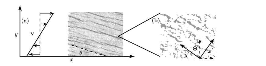
The dynamic origins of melt-preferred orientation remain poorly understood. In laboratory deformation experiments, melt pockets become elongated such that in cross section, they have a long axis and a short axis, as shown in Fig. 1. Coherent alignment of the long axes of melt pockets results from an unknown combination of the instantaneous stress (Takei and Holtzman, 2009a) and the finite strain (Daines and Kohlstedt, 1997; Jung and Waff, 1998). The latter acts to align olivine grains, which have anisotropic surface energy and hence anisotropic wetting affinity. If the deviatoric stress is the dominant forcing of MPO, we would expect melt pockets to be in instantaneous alignment, with their long axes perpendicular to the direction of maximum tension (the $\sigma_{3}$-direction). We can generalise this, however, and investigate the consequences of MPO alignment in terms of the angle $\Theta$ between the shear plane and the normal to the long axis of a melt pocket.

This angle is used to define a rotated coordinate system as in Fig. 1. The $x^{\prime}$-direction is normal to melt pockets and expected to have a low permeability. The $y^{\prime}$-direction is parallel to melt pockets (and in the plane defined by the eigenvectors corresponding to $\sigma_{1}$ and $\sigma_{3}$); this direction is expected to have a high permeability.

We quantify these expectations with the tensor $\mathbf{A}^{\prime}$ in the rotated coordinate system,

$$\mathbf{A^{\prime}}=\left(\begin{array}[]{cc}k_{\perp}&0\\ 0&k_{\parallel}\end{array}\right),$$ (9)

where $k_{\parallel}\geq 1$ is the permeability enhancement along $y^{\prime}$ and $0\leq k_{\perp}\leq 1$ is the reduction along $x^{\prime}$. A symmetry argument (Appendix A) shows that $\mathbf{A^{\prime}}$ must be diagonal. Then, by rotating from the primed to the unprimed coordinates, the anisotropy matrix is written as

$$\mathbf{A}=\mathbf{R}\mathbf{A^{\prime}}\mathbf{R}^{T}=\left(\begin{array}[]{cc}k_{\perp}\cos^{2}\Theta+k_{\parallel}\sin^{2}\Theta&(k_{\perp}-k_{\parallel})\cos\Theta\sin\Theta\\ (k_{\perp}-k_{\parallel})\cos\Theta\sin\Theta&k_{\perp}\sin^{2}\Theta+k_{\parallel}\cos^{2}\Theta\end{array}\right).$$ (12)

Here we could factor out $k_{\parallel}$, for example, and lump it with $K_{0}$, reducing by one the number of parameters in the problem. However, since we have non-dimensionalised lengths with the compaction length (and hence with $K_{0}$), this would obscure the role of permeability enhancement parallel to MPO.

Much of the work below is in understanding the behaviour of solutions to the system (6) under different assumptions for the values of $k_{\perp}$, $k_{\parallel}$, and $\Theta$ in the tensor (12). A list of the key non-dimensional symbols used in this manuscript is provided in table 1.

Symbol	meaning	equation, value, or range
$\boldsymbol{x}$	position
$t$	time
$P$	liquid pressure
$\mathbf{v}$	velocity
$\phi$	porosity
$\mathcal{C}$	compaction rate	$\boldsymbol{\nabla}\cdot\mathbf{v}$
$\eta_{\phi}$	shear viscosity	$\eta_{\phi}=\exp\left[-\lambda(\phi-\phi_{0})\right]$
$\zeta_{\phi}$	bulk viscosity	$\zeta_{\phi}=r_{\zeta}\eta_{\phi}$
$\lambda$	porosity-weakening exponent	27
$r_{\zeta}$	viscosity ratio	5/3
$\phi_{0}$	reference porosity	0.05
$\ell$	permeability exponent	3
$\mathbf{A}$	permeability anisotropy tensor	eqn. (12)
$k_{\parallel}$	MPO-parallel permeability factor	1–200
$k_{\perp}$	MPO-perpendicular permeability factor	0.005–1
$\Theta$	angle of MPO to shear plane	$0^{\circ}$–$90^{\circ}$
$\theta$	angle of perturbation wavevector to shear plane	$0^{\circ}$–$180^{\circ}$
$\epsilon$	very small number	$\ll 1$
$s,\dot{s}$	perturbation amplitude, growth rate	eqn. (16), (17)
$\boldsymbol{\kappa},\kappa$	perturbation wave-vector, magnitude	$\boldsymbol{\kappa}=\kappa\left(\sin\theta,\cos\theta\right)$

Table 1: Dimensionless symbols and their meaning.

4 Linearised stability analysis

Equations (6) form a coupled, non-linear, time-dependent system. To make analytical progress, we follow previous workers (e.g Spiegelman, 2003; Katz et al., 2006) and employ a linearised stability analysis. We expand the problem variables in a power-series of $\epsilon\ll 1$ and truncate after first order,

$$\left\{\begin{array}[]{l}\phi=\phi_{0}+\epsilon\phi_{1}\left(\boldsymbol{x},t\right),\\ P=P_{0}+\epsilon P_{1}\left(\boldsymbol{x},t\right),\\ \mathbf{v}=\mathbf{v}^{\left(0\right)}\left(\boldsymbol{x}\right)+\epsilon\mathbf{v}^{\left(1\right)}\left(\boldsymbol{x},t\right),\\ \mathcal{C}=\mathcal{C}_{0}+\epsilon\mathcal{C}_{1}\left(\boldsymbol{x},t\right).\end{array}\right.$$ (13)

Terms of order $\epsilon^{0}$ are taken to define the base-state about which we perturb. The expansion of porosity can be used to express the nondimensional permeability and viscosity to first order as

$$\left(\phi/\phi_{0}\right)^{\ell} =1+\epsilon\ell\phi_{1}/\phi_{0}$$ (14a)

$$\textrm{e}^{-\lambda(\phi-\phi_{0})} =1-\epsilon\lambda\phi_{1}.$$ (14b)

Substituting (13) and (14) into (6) and requiring terms to balance at each order allows us to derive two systems of linear equations at $\mathcal{O}(\epsilon^{0})$ and $\mathcal{O}(\epsilon^{1})$. We assume that the leading-order porosity $\phi_{0}$ is uniform and that the flow is simple shear with $\mathbf{v}^{(0)}=(\dot{\gamma}y,0)$. The uniform, leading-order viscosity and permeability therefore result in $\mathcal{C}_{0}=0$ and $P_{0}=\textrm{const}$.

The first order balance of equations (6) becomes

$$\partial_{t}{\phi_{1}} =(1-\phi_{0})\mathcal{C}_{1}-\mathbf{v}^{(0)}\cdot\boldsymbol{\nabla}\phi_{1},$$ (15a)

$$\mathcal{C}_{1} =(r_{\zeta}+4/3)^{-1}\boldsymbol{\nabla}\cdot\left[\mathbf{A}\boldsymbol{\nabla}P_{1}\right],$$ (15b)

$$\boldsymbol{\nabla}P_{1} =\boldsymbol{\nabla}\cdot\left[\boldsymbol{\nabla}\mathbf{v}^{(1)}+(\boldsymbol{\nabla}\mathbf{v}^{(1)})^{T}\right]+(r_{\zeta}-2/3)\boldsymbol{\nabla}\mathcal{C}_{1}-\lambda\boldsymbol{\nabla}\cdot\left[\phi_{1}\left(\boldsymbol{\nabla}\mathbf{v}^{(0)}+(\boldsymbol{\nabla}\mathbf{v}^{(0)})^{T}\right)\right].$$ (15c)

We consider harmonic porosity perturbations that are advected by the background simple shear

$$\phi_{1}=\exp\left[i\boldsymbol{\kappa}\cdot\left(\boldsymbol{x}-\int_{0}^{t}\mathbf{v}^{(0)}\text{d}t\right)+s(t)\right],$$ (16)

where $\exp s(t)$ is the time-dependent amplitude and the wave-vector is given as $\boldsymbol{\kappa}=\left(\kappa_{x},\kappa_{y}\right)=\kappa\left(\sin\theta,\cos\theta\right)$. Hence $\theta$ represents the angle between the perturbation wave vector $\boldsymbol{\kappa}$ and the $y$-axis or, equivalently, between the perturbation wavefronts and the shear plane.

This linearised system (15) can be solved, along with (16), to obtain the growth rate (details in Appendix B)

$$\dot{s}=\lambda\frac{1-\phi_{0}}{r_{\zeta}+4/3}\sin{2\theta}\frac{\left\langle\boldsymbol{\kappa},\mathbf{A}\boldsymbol{\kappa}\right\rangle}{1+\left\langle\boldsymbol{\kappa},\mathbf{A}\boldsymbol{\kappa}\right\rangle},$$ (17)

where the inner product notation means $\left\langle\boldsymbol{\kappa},\mathbf{A}\boldsymbol{\kappa}\right\rangle=\sum_{i}\limits\sum_{j}\limits\kappa_{i}A_{ij}\kappa_{j}$.

For isotropic permeability $k_{\perp}=k_{\parallel}=1$; then from equation (12), $\mathbf{A}$ reduces to the identity matrix. In this case, the growth rate is identical to that calculated by Spiegelman (2003) for isotropic permeability (and viscosity). Further, in the limit of vanishing perturbation wavelength $\kappa\to\infty$ (where $\kappa=|\boldsymbol{\kappa}|$), the ratio $\left\langle\boldsymbol{\kappa},\mathbf{A}\boldsymbol{\kappa}\right\rangle/(1+\left\langle\boldsymbol{\kappa},\mathbf{A}\boldsymbol{\kappa}\right\rangle)\to 1$ and so the growth rate again reduces to that of the isotropic case. In contrast, the limit $\kappa=0$ has zero growth rate. It can be shown (Appendix B) that the greatest sensitivity to the anisotropy of permeability occurs where $2\pi/\kappa\sim 1$ or, in dimensional terms, when the wavelength of the instability is approximately equal to the compaction length.

Figure 2: Anisotropy factor $F$ as a function of $\theta+\Theta$ for $\kappa=1$ and various values of $k_{\parallel}$. (a) $k_{\perp}=0.5$. (b) $k_{\perp}=0.005$.

For a permeability matrix $\mathbf{A}$ from equation (12) we can expand and simplify to obtain

$$\left\langle\boldsymbol{\kappa},\mathbf{A}\boldsymbol{\kappa}\right\rangle=\kappa^{2}\left[k_{\parallel}-(k_{\parallel}-k_{\perp})\sin^{2}(\theta+\Theta)\right].$$

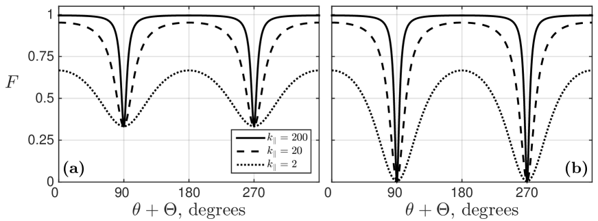
Hence from equation (17), we are interested in the behaviour of the factor

$$F=\frac{\kappa^{2}\left[k_{\parallel}-(k_{\parallel}-k_{\perp})\sin^{2}(\theta+\Theta)\right]}{1+\kappa^{2}\left[k_{\parallel}-(k_{\parallel}-k_{\perp})\sin^{2}(\theta+\Theta)\right]}.$$ (18)

that modifies the isotropic growth rate. $F$ is plotted in Fig. 2 as a function of $\theta+\Theta$ for $\kappa=1$ and various values of $k_{\parallel}$ and $k_{\perp}$. MPO is parallel to porosity perturbations when $\theta+\Theta=90^{\circ}$ or $270^{\circ}$. At these two angles, the reduced permeability $k_{\perp}$ in the MPO-perpendicular direction controls the flow of melt perpendicular to bands and causes a minimum in $F$. With $k_{\perp}\to 0$, melt cannot segregate in the direction perpendicular to MPO, and hence it cannot feed bands that are oriented parallel to MPO. When $\theta+\Theta\neq 90^{\circ}$ or $270^{\circ}$, values of $k_{\parallel}>1$ facilitate segregation of melt into (or out of) perturbations.

Although permeability can promote or impede melt transport, it does not drive melt transport. In this context, it is important to note that in the linearised analysis, the permeability does not multiply any zeroth-order fields and hence perturbations to the permeability play no role in the first-order balance (15). Only anisotropy of the zeroth-order permeability affects the growth rate of porosity perturbations. Here we assume that MPO (and hence anisotropic permeability) emerges on a much shorter time scale than melt redistribution, so the leading-order MPO is in equilibrium with the leading-order stress state. This assumption is consistent with grain-scale models (Hier-Majumder, 2011) as well as experimental observations (Takei, 2010; Zimmerman et al., 1999). Other experiments indicate that the strength of MPO increases with the amount of time that the stress is applied (Daines and Kohlstedt, 1997). Furthermore, the local stress state is affected by the segregation of melt into bands (e.g. Takei and Katz, 2015), which could modify the MPO and the permeability. However, in the context of linearised analysis, this would not appear at leading order and hence would not modify our results.

Equation (17) shows that the growth-rate of perturbations depends on the product of $F$ with $\sin 2\theta$, where the latter represents the deviatoric stress (tension positive) that drives melt segregation. In the absence of anisotropic permeability, $\sin 2\theta$ is the sole angular dependence of the growth rate and bands are predicted to grow fastest at $45^{\circ}$ to the shear plane. We next explore how and when $F$ modifies this prediction.

4.1 MPO orientation and growth rate

We return to (17) and consider the role of the orientation of anisotropy $\Theta$. Within the limitations of linearised analysis, it is the porosity perturbation with the largest instantaneous growth rate that is predicted to dominate after finite time, and hence to be expressed by the physical system. We are therefore interested in the angle $\theta^{*}$ at which the growth rate reaches its maximum, $\dot{s}^{*}$. Since the growth rate is most sensitive to anisotropy at $\kappa\sim 1$, we consider only $\kappa=1$ in this section; this constraint is relaxed in the following sections.

Figure 3: Growth-rate $\dot{s}$ versus $\theta$ for various values of anisotropy angle $\Theta$. Each curve is calculated with $k_{\perp}=0.005$, $k_{\parallel}=2$.

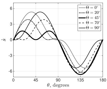
Fig. 3 shows the growth rate versus $\theta$ for a set of values of anisotropy angle $\Theta$. Independent of any imposed anisotropy, perturbation growth is driven by tension across a high-porosity, viscously weak band (Stevenson, 1989). As band angles rotate into directions parallel or perpendicular to the shear plane, this tension vanishes and the growth rate goes to zero (Spiegelman, 2003); this is why all curves in Fig. 3 cross $\dot{s}=0$ at $0^{\circ}$ and $90^{\circ}$. Anisotropy of permeability modifies the $\sin 2\theta$ dependence of growth-rate predicted by Spiegelman (2003). As $\Theta$ is increased from its smallest value, a local minimum in the positive growth rates appears in the range $0^{\circ}\leq\theta\leq 90^{\circ}$. This minimum exists at the angle where perturbation wavefronts are parallel to MPO, $\theta=90^{\circ}-\Theta$. For the case of $\Theta=45^{\circ}$, the minimum occurs at $\theta=45^{\circ}$ and we find two peaks of equal growth rate, one at an angle lower than $45^{\circ}$ and one higher. Katz et al. (2006) show that although the two perturbation angles have the same instantaneous growth rate, it is the lower-angle perturbation that dominates, since the high-angle band is rotated more rapidly by the background, simple-shear flow out of favourable orientation for growth (eqn. (16)).

4.2 Perturbation wavelength and growth rate

As in previous work on isotropic permeability (e.g. Stevenson, 1989), the growth rate in equation (17) depends on the wavelength of perturbations relative to the compaction length. Fig. 4(a) plots growth rate against the log of perturbation wavelength for the angle $\theta^{*}$ that has maximum growth rate. Here, we consider only MPO aligned at $\Theta=45^{\circ}$. For perturbation wavelengths much larger than the compaction length, the growth rate of perturbations drops to zero. Over these distances, pressure gradients associated with variation in viscosity are small and cannot drive melt segregation and differential compaction.

Figure 4: The effect of perturbation wavelength $2\pi/\kappa$ when $\Theta=45^{\circ}$, $k_{\perp}=0.005$ and $k_{\parallel}=2$. (a) Maximum growth rate, $\dot{s}^{*}$, against log-wavelength. (b) $\theta^{*}$ against log-wavelength. The angle of both the low- and the high-angle growth peaks is plotted.

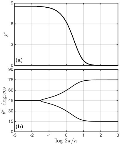
Looking instead at wavelengths much smaller than the compaction length, Fig. 4(a) indicates that there is no wavelength selection by the growth rate. At vanishingly small perturbation wavelengths, the resistance to segregation by Darcy drag is negligible. This highly local segregation is insensitive to the permeability; its orientation of maximal growth rate is therefore determined entirely by the orientation of the stress tensor and hence by $\sin 2\theta$. Fig. 4(b) plots $\theta^{*}$ as a function of perturbation wavelength; it confirms that at wavelengths smaller than a tenth of the compaction length $\theta^{*}=45^{\circ}$, as in the isotropic case. For increasing wavelength, anisotropy of permeability plays an increasing role; the $45^{\circ}$ growth-rate peaks splits into two peaks of equal height (as in Fig. 3 for $\Theta=45^{\circ}$). However, this split occurs as the growth rate declines to zero. Therefore, in a full, nonlinear solution to the governing equations that is initialised with a broadband spectrum of perturbations, the growth of shorter-wavelength perturbations would dominate the porosity field. These would likely appear at $\sim 45^{\circ}$. However Butler (2010) showed that the wavelength of high porosity bands in numerical simulations increases as the system evolves, due to the kinematics of the background flow. He explained that bands grow, rotate, and widen until wavelengths are similar to one compaction length. This is, as we have shown, the length scale at which anisotropic permeability has a significant effect on band angles.

It is also important to note, however, that application of the present model to arbitrarily small wavelength is invalid because the continuum assumptions hold only at length-scales much larger than the solid grains. Indeed if we consider the formation of “bands” at the grain scale, the distribution of melt is indistinguishable from melt-preferred orientation. So for a variation in porosity to be considered a melt-rich band, the variation must take place over a length-scale on which the concept of porosity is well defined; i.e. a large multiple of the mean grain size. Such wavelength are, in fact, observed in experiments (Holtzman et al., 2003; King et al., 2010) indicating that either the initial variations of porosity are concentrated at intermediate or larger scales, or that the non-linear system is regularised over finite time by some process that has not been included in the theory above. Possible examples of the latter are surface-energy-driven flow (Bercovici and Rudge, 2015) and dissolution/transport/precipitation due to gradients in chemical potential (Takei and Hier-Majumder, 2009).

4.3 The conditions for low-angle bands

To search for anisotropy conditions conducive to formation of low-angle bands, we map out the effect of anisotropy on $\theta^{*}$. Fig. 5 displays contours of $\theta^{*}$ and is coloured according to the corresponding (maximum) growth rate $\dot{s}^{*}$, for fixed $\kappa=1$. This is done in the space of $\left(-\log k_{\perp},\log k_{\parallel}\right)$ because $k_{\perp}$ ranges between zero and one, while $k_{\parallel}$ is greater than or equal to one. For any point in this space at which $\dot{s}$ has two maxima with equal rates, we select the one at smaller $\theta$, corresponding to bands that are more slowly rotated by the base-state flow. In these plots, the lower-left corner corresponds to the isotropic case (where $\theta^{*}=45^{\circ}$) while the top-right corner corresponds to the case with strong anisotropy.

Figure 5: Contours of $\theta^{*}$ (degrees) superimposed on a color-scale plot of $\dot{s}^{*}$ for $\kappa=1$. (a) $\Theta=20^{\circ}$. (b) $\Theta=45^{\circ}$. (c) $\Theta=70^{\circ}$.

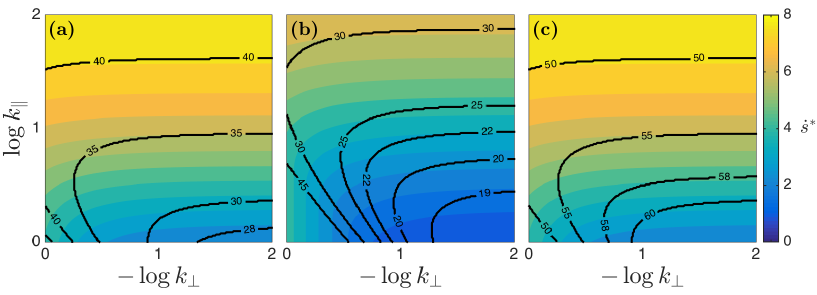
Fig. 5 demonstrates that $\theta^{*}$ is most effectively reduced by a sharp decrease of $k_{\perp}$ with little or no change in $k_{\parallel}$. Panel (b) uses $\Theta=45^{\circ}$ and shows that in this case, $\theta^{*}$ can be lowered to below $20^{\circ}$ by imposing $\kappa\sim 1$, $k_{\parallel}\sim 1$, and $k_{\perp}\to 0$. Under these conditions the predicted angles are consistent with bands observed in experiments, however $\dot{s}$ is low and so rotation due to the background flow is likely to result in bands observed at higher angles than the angle of maximal instantaneous growth rate. Panels (a) and (c), however, show that for $\Theta=20^{\circ}$ and $\Theta=70^{\circ}$, $\theta^{*}$ cannot be lowered to angles consistent with the experimental band angles.

All three panels of Fig. 5 show that away from the origin, the maximal growth rate $\dot{s}^{*}$ increases with $k_{\parallel}$ and is nearly independent of $k_{\perp}$. Close to the origin, where the permeability is approximately isotropic, the growth rate does depend on $k_{\perp}$ (see especially panel (b)). For bands to grow, the melt segregation velocity must have a component normal to the perturbation wavefronts. And as we have seen above, growth rate is sensitive to the orientation of perturbations with respect to MPO and to the perturbation wavelength relative to the compaction length. A simple heuristic that combines these dependencies is the non-dimensional compaction length in the direction normal to perturbation wavefronts of the fastest-growing perturbation. We define this as

$$\delta^{*}\equiv\sqrt{\left\langle\boldsymbol{\kappa}^{*},\mathbf{A}\boldsymbol{\kappa}^{*}\right\rangle}=\kappa\sqrt{k_{\parallel}-(k_{\parallel}-k_{\perp})\sin^{2}(\theta^{*}+\Theta)}.$$

This definition requires that when MPO is parallel to maximally growing perturbations ($\theta^{*}+\Theta=90^{\circ}$ or $270^{\circ}$), the compaction length across bands is controlled by $\sqrt{k_{\perp}}$, whereas when MPO is normal to these perturbations, the compaction length is controlled by $\sqrt{k_{\parallel}}$. Returning to Fig. 5, far from the origin we have $k_{\parallel}\gg k_{\perp}$ and $\sin^{2}(\theta^{*}+\Theta)\neq 1$, so $\delta^{*}$ (and hence $\dot{s}^{*}$) is primarily dependent on $k_{\parallel}$. Near the origin, $k_{\parallel}\approx k_{\perp}\approx 1$ and so $\delta^{*}$ depends on both permeability parameters. In panel (b) near the origin, we have the special case of $\theta^{*}=\Theta=45^{\circ}$; hence $\delta^{*}=\sqrt{k_{\perp}}$ so $\dot{s}^{*}$ depends only on $k_{\perp}$ here.

5 Numerical simulations

The linearised stability analysis presented above is valid at infinitessimal strains and only for the plane-wave perturbations considered. Numerical solutions discussed in this section allow us to verify and extend the linearised analysis. We solve the system (6) with permeability tensor (12) and shear and compaction viscosity as specified above in §2. The domain is rectangular with height $H$ and boundary conditions of tangengial velocity $\mathbf{v}=\pm\tfrac{1}{2}\dot{\gamma}H\hat{\boldsymbol{x}}$ (dimensional; positive velocity on the top boundary) and impermeability $\hat{\boldsymbol{y}}\cdot\mathbf{K}=\boldsymbol{0}$ imposed on the top and bottom boundaries (the domain is periodic in the $x$ direction). Spatial derivatives are discretised on a Cartesian, fully staggered grid with square cells. A semi-implicit, Crank-Nicolson scheme is used to discretise time, and the hyperbolic equation for porosity evolution is solved separately from the elliptic system in a Picard loop with two iterations at each time-step. The solutions are obtained in the context of the Portable, Extensible Toolkit for Scientific Computation (PETSc, Balay et al., 2001, 2004; Katz et al., 2007). Full details and references are provided by Katz and Takei (2013).

Numerical simulations of band formation with isotropic permeability are documented in the literature (e.g. Katz et al., 2006; Katz and Takei, 2013) and not repeated here. Instead, we consider simulations in which the anisotropy is fixed at $\Theta=45^{\circ}$, $k_{\perp}=0.005$, and $k_{\parallel}=2$; we vary the ratio of the smallest perturbation wavelength to the compaction length. All simulations are initialised with the identical porosity field, shown in Fig. 6(a). This field is constructed as $\phi(\boldsymbol{x},t=0)=\phi_{0}+\epsilon\phi_{1}(\boldsymbol{x})$, where $\phi_{0}=0.05$ and $\epsilon=0.005$. $\phi_{1}(\boldsymbol{x})$ is a smooth, random field with unit amplitude, generated by filtering grid-scale white noise to remove variation at wavelengths below $H/10$. Hence the smallest perturbation wavelength is $2\pi/\kappa_{\text{max}}=H/(10\delta)$, in non-dimensional terms that correspond to the abscissa in Fig. 4. A suite of simulations at different values of compaction length $\delta$ was run to compare the distribution of angles for a broadband perturbation.

If the prediction from the linearised stability analysis holds, we expect simulations to produce bands at low ($\sim$$20^{\circ}$) and high ($\sim$$70^{\circ}$) angles when the minimum perturbation wavelength is greater than the compaction length, $H/(10\delta)\gtrsim 1$. In contrast, when the minimum perturbation wavelength is smaller than the compaction length, we expect a transition to $\theta\gtrsim 45^{\circ}$. These systematics are discernable in Fig. 4.

Figure 6: Results from numerical solutions of (6) with permeability tensor (12) on a 1200$\times$600 grid. Parameter values are $k_{\perp}=0.005$, $k_{\parallel}=2$, $\Theta=45^{\circ}$. The coordinate axes $(x,y)$ have been rescaled with $\delta/H$, where $\delta$ is the compaction length and $H$ is the domain height. (a) The initial porosity field with mean $\phi_{0}=0.05$ and random perturbation of amplitude $\epsilon=\tfrac{1}{10}\phi_{0}$. The perturbation is white noise, filtered to remove wavelengths smaller than $1/10^{\text{th}}$ the domain height. This field is used to initialise all simulations. (b) The porosity field at strain $\gamma=0.4$ from a simulation with the compaction length chosen as $\delta=0.05H$ such that $\log 2\pi/\kappa_{\text{max}}=0.3$. (c) Spectral power binned by perturbation wavefront-angle $\theta$ to the shear plane (after Katz et al., 2006) for the porosity field at $\gamma=0.4$ from simulations with values of $\delta$. Curves are normalised to have unit maximum.

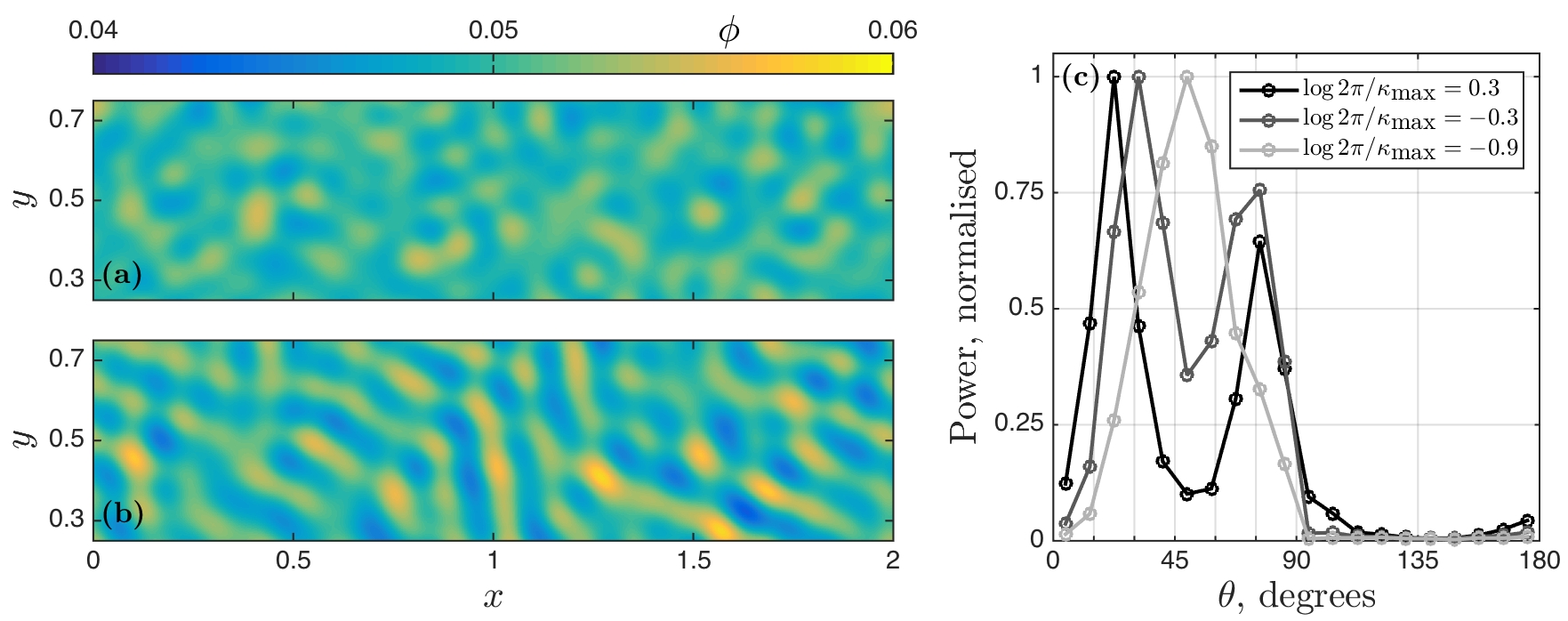
Fig. 6(b) shows the porosity field from a simulation with $\delta=0.05H$ (and thus $\log 2\pi/\kappa_{\text{max}}=0.3$) after a strain of $\gamma=0.4$. The porosity field, which was initially as shown in panel (a) of the same figure, has evolved to form low- and high-angle porosity bands. The angles of these features are characterised in the power spectrum shown in panel (c). Here, spectral power from a two-dimensional Fourier transform is binned according to the angle that wavefronts make with the shear plane. The black curve represents the case of perturbations with a minimum wavelength that is larger than the compaction length. It is peaked at $\sim$$22^{\circ}$ to the shear plane, with a secondary peak at $\sim$$75^{\circ}$. This asymmetry is in contrast with the equal heights of growth-rate peaks in Fig. 3 for $\Theta=45^{\circ}$. However, the relatively smaller height of the high-angle peak is expected because under simple-shear deformation, high-angle features are rotated more rapidly than low-angle features; this means that they spend less time in optimal orientation for growth (Katz et al., 2006).

Fig. 6(c) compares the angular spectra of simulations with three different values of $\log 2\pi/\kappa_{\text{max}}$. As the minimum wavelength of perturbation decreases from longer than to shorter than the compaction length, the dominant band orientation rotates to higher angle. For $\log 2\pi/\kappa_{\text{max}}\sim-1$, the low- and high-angle peaks have merged into a single peak at about $45^{\circ}$ (slightly higher due to rotation). This confirms the prediction of linearised analysis over finite strains.

6 Discussion and conclusion

The foregoing theory and results extend the equations of two-phase, magma/mantle dynamics to include anisotropic permeability. Anisotropic permeability is likely to arise as a consequence of melt-preferred orientation, the coherent alignment of melt pockets between solid grains. This alignment may be a consequence of finite strain or of deviatoric stress, or some combination of the two. Although we don’t model details of the two-phase microstructure (Hersum, 2008), we assume that MPO is a consequence of deviatoric stress, develops instantaneously, and is thus active at $t=0$ (Takei and Holtzman, 2009a). We postulate a simple anisotropy tensor with two eigenvalues representing the MPO-parallel and MPO-perpendicular permeabilities. An angle between the shear plane and the perpendicular to MPO then becomes the third parameter in the anisotropy model.

To understand the behaviour of the system of governing equations and constitutive laws, we perform linearised stability analysis and obtain numerical solutions. We explore the $(k_{\parallel},k_{\perp},\Theta)$ parameter space of the anisotropy model with a particular focus on $\Theta=45^{\circ}$, representing MPO aligned perpendicular to the maximum tensile direction of the deviatoric stress tensor.

For perturbations with wavelengths approximately equal to the compaction length, anisotropic permeability modifies the angular dependence of the perturbation growth rate. It suppresses the growth of high-porosity bands when those bands are in or near alignment with the MPO (high-permeability) direction. This is because melt that segregates into MPO-parallel bands must overcome the reduced permeability perpendicular to MPO. For $\Theta=45^{\circ}$, MPO is aligned normal to the direction of maximum tensile stress, and hence the reduced permeability resists band growth at precisely the angle that would be optimal in the absence of anisotropy. In this case, the symmetric peaks in growth rate arise at angles where the product of band-perpendicular tension and band-perpendicular permeability is maximised. This angle selection, however, depends on the wavelength of perturbation. Wavelengths much longer than the compaction length do not generate sufficient pressure gradients to cause melt segregation and band growth; wavelengths much shorter than the compaction length are unhindered by the extremely short pathways of melt segregation (over which they experience the anisotropy), and hence grow optimally at $45^{\circ}$.

Of particular interest in this exploration is the question of whether anisotropy of permeability can give rise to bands of high porosity that are oriented at low angle ($\lesssim 20^{\circ}$) to the shear plane, as observed in laboratory experiments. Our analysis predicts that it is possible, under certain conditions (i.e. $\Theta\sim 45^{\circ},\,2\pi/\kappa\sim 1,\,k_{\parallel}/k_{\perp}\gg 1$), to obtain bands oriented at the low angles that are consistent with experiments. These are fairly restrictive conditions. The requirement that initial porosity perturbations be of a wavelength that is greater than about one compaction length seems especially significant. Also, the angle of MPO that is typically measured under relevant experimental conditions is closer to $\Theta=30^{\circ}$, as opposed to $45^{\circ}$, though there is no accepted explanation for this.

On the other hand, there are arguments for the conditions above to be met, in which case anisotropic permeability might play a role in shaping and orienting the high porosity bands. Firstly, bands observed in experiments tend not to have wavelengths of a much smaller scale than the compaction length (Holtzman and Kohlstedt, 2007). This suggest that either the initial porosity variations are indeed concentrated at a relatively large scale or, as briefly considered above, the non-linear system is regularised by a process that occurs at a scale close to the compaction length. This could occur by surface tension acting over a diffuse interface (Bercovici and Rudge, 2015) or by diffusion of chemical components (Takei and Hier-Majumder, 2009). Secondly, the argument given by Butler (2010) for the growth of band wavelengths suggests that the porosity variations would evolve kinematically to a length scale comparable to the compaction length and hence the system would become susceptible to the effects of anisotropic permeability.

Although anisotropic permeability in the form discussed here may not independently explain the low angle of porosity bands in laboratory experiments, it may still be relevant in shaping the dynamics of those experiments, or of partially molten rocks more generally. Anisotropy of permeability may, for example, affect the trajectories of rising magma beneath mid-ocean ridges (Morgan, 1987) or melt segregation in magma chambers (Bergantz, 1995); in industrial processes, it has implications for macrosegregation during solidification (e.g. Yoo and Viskanta, 1992). More work is therefore needed to understand the consequences of anisotropy as well as the causes. In this latter category: How can melt-preferred orientation be quantitatively related to permeability? And, even more fundamentally, what is the energetic or mechanical cause for melt-preferred orientation?

Acknowledgements

The authors thank S. Butler and an anonymous reviewer for insightful comments. The research leading to these results has received funding from the European Research Council (ERC) under the European Union’s Seventh Framework Programme (FP7/2007–2013)/ERC grant agreement 279925. JT-W was supported for summer 2014 by as Research Experience Placement grant from the Natural Environment Research Council of the Research Councils UK. RFK is grateful for the support of the Leverhulme Trust. Numerical solutions were computed at the Advanced Research Computing facility of the University of Oxford.

Appendix A Diagonality of permeability tensor

To understand why the permeability tensor $\mathbf{A}$ must be diagonal when expressed in a coordinate system aligned with MPO, consider equation (1c) with uniform porosity $\phi=\phi_{0}$ and permeability given by equation (4),

$$\phi_{0}\left(\boldsymbol{v}^{S}-\boldsymbol{v}^{L}\right)=\frac{K_{0}}{\mu}\mathbf{A}\boldsymbol{\nabla}p^{L}.$$ (A.1)

We now adopt the primed coordinate system of Figs. 1 and 7 that is aligned with the melt-preferred orientation. Making no assumptions about the form of the permeability tensor, equation (A.1) becomes

$$\boldsymbol{q}=\frac{K_{0}}{\mu}\left(\begin{array}[]{cc}k_{\perp}&k_{\times_{1}}\\ k_{\times_{2}}&k_{\parallel}\end{array}\right)\boldsymbol{\nabla}p^{L},$$ (A.4)

where $\boldsymbol{q}=\phi_{0}(\boldsymbol{v}^{S}-\boldsymbol{v}^{L})$ is the segregation flux. For a unit pressure gradient, $\boldsymbol{\nabla}p^{L}=(0,1)$, applied in the $y^{\prime}$-direction we have

$$\boldsymbol{q}=\frac{K_{0}}{\mu}(k_{\times_{1}}\hat{\boldsymbol{x}}^{\prime}+k_{\parallel}\hat{\boldsymbol{y}}^{\prime})$$ (A.5)

with an $x^{\prime}$-component $q_{x^{\prime}}$ proportional to $k_{\times_{1}}$.

Figure 7: Reflection of MPO in $y^{\prime}$–axis

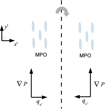
If we reflect in an axis parallel to the $y^{\prime}$-direction, as shown in Fig. 7, the pressure gradient is unchanged but the cross-MPO segregation $q_{x^{\prime}}$ becomes proportional to $-k_{\times_{1}}$. However, the melt-pocket structure in Fig. 1 is unchanged and so the permeability tensor should not change. Hence the segregation obtained from (A.4) is still given by equation (A.5) and we have $k_{\times_{1}}=-k_{\times_{1}}=0$, and by a similar argument $k_{\times_{2}}=0$.

Appendix B Solving the linearised equations for $\dot{s}$

Because the system of equations that governs the perturbation quantities is linear, we are able to relate the other variables to $\phi_{1}$ via unknown coefficients,

$$\mathbf{v}^{(1)}=\tilde{\mathbf{v}}\phi_{1},\hskip 11.38109ptP_{1}=\tilde{P}\phi_{1},$$ (B.1)

The order-$\epsilon$ balance derived from equation (6a) then gives

$$\dfrac{\partial{\phi_{1}}}{\partial{t}}=\left(1-\phi_{0}\right)\tilde{\mathbf{v}}\cdot\boldsymbol{\nabla}\phi_{1}-\mathbf{v}^{(0)}\cdot\boldsymbol{\nabla}\phi_{1}.$$ (B.2)

Expanding time and space derivatives using (16) and rearranging, equation (B.2) becomes an equation for the growth rate

$$\dot{s}=\left(1-\phi_{0}\right)i\boldsymbol{\kappa}\cdot\tilde{\mathbf{v}}=\left(1-\phi_{0}\right)\mathcal{C}_{1}/\phi_{1}.$$ (B.3)

Substituting $\mathbf{v}^{(0)}=(Y,0)$, $\mathbf{v}^{(1)}=\tilde{\mathbf{v}}\phi_{1}$ and $P_{1}=\tilde{P}\phi_{1}$ into the $x$ and $y$ components of equation (15c) gives

$$\tilde{P}\kappa_{x} =i\left[\left(r_{\zeta}+4/3\right)\kappa_{x}^{2}\tilde{V_{x}}+\left(r_{\zeta}+1/3\right)\kappa_{x}\kappa_{y}\tilde{V_{y}}+\kappa_{y}^{2}\tilde{V_{x}}\right]-\lambda\kappa_{y},$$ (B.4a)

$$\tilde{P}\kappa_{y} =i\left[\left(r_{\zeta}+4/3\right)\kappa_{y}^{2}\tilde{V_{y}}+\left(r_{\zeta}+1/3\right)\kappa_{x}\kappa_{y}\tilde{V_{x}}+\kappa_{x}^{2}\tilde{V_{y}}\right]-\lambda\kappa_{x},$$ (B.4b)

which can be combined using $\kappa_{x}^{2}+\kappa_{y}^{2}=\kappa^{2}$ to obtain

$$\tilde{P} =i\left(r_{\zeta}+4/3\right)\left(\kappa_{x}\tilde{V_{x}}+\kappa_{y}\tilde{V_{y}}\right)-2\frac{\kappa_{x}\kappa_{y}}{\kappa^{2}}\lambda$$

$$=\left(r_{\zeta}+4/3\right)\mathcal{C}_{1}/\phi_{1}-\lambda\sin{2\theta}.$$ (B.5)

By substituting this into equation (15b) we obtain

$$\mathcal{C}_{1} =\frac{1}{r_{\zeta}+4/3}\boldsymbol{\nabla}\cdot\left(i\tilde{P}\mathbf{A}\boldsymbol{\kappa}\phi_{1}\right)$$

$$=-\frac{\tilde{P}}{r_{\zeta}+4/3}\left\langle\boldsymbol{\kappa},\mathbf{A}\boldsymbol{\kappa}\right\rangle\phi_{1}$$

$$=-\left\langle\boldsymbol{\kappa},\mathbf{A}\boldsymbol{\kappa}\right\rangle\mathcal{C}_{1}+\frac{\lambda\sin{2\theta}}{r_{\zeta}+4/3}\left\langle\boldsymbol{\kappa},\mathbf{A}\boldsymbol{\kappa}\right\rangle\phi_{1},$$ (B.6)

where the inner product notation means $\left\langle\boldsymbol{\kappa},\mathbf{A}\boldsymbol{\kappa}\right\rangle=\sum_{i}\limits\sum_{j}\limits\kappa_{i}A_{ij}\kappa_{j}$. This provides an expression for $\mathcal{C}_{1}/\phi_{1}$ that, when substituted into (B.3), gives the growth rate

$$\dot{s}=\lambda(r_{\zeta}+4/3)^{-1}\left(1-\phi_{0}\right)\sin{2\theta}\frac{\left\langle\boldsymbol{\kappa},\mathbf{A}\boldsymbol{\kappa}\right\rangle}{1+\left\langle\boldsymbol{\kappa},\mathbf{A}\boldsymbol{\kappa}\right\rangle}.$$ (B.7)

To understand the role of perturbation wavelength in controlling the growth rate we consider the anisotropy factor

$$F=\frac{\left\langle\boldsymbol{\kappa},\mathbf{A}\boldsymbol{\kappa}\right\rangle}{1+\left\langle\boldsymbol{\kappa},\mathbf{A}\boldsymbol{\kappa}\right\rangle}=\frac{\kappa^{2}\left[k_{\parallel}-(k_{\parallel}-k_{\perp})\sin^{2}(\theta+\Theta)\right]}{1+\kappa^{2}\left[k_{\parallel}-(k_{\parallel}-k_{\perp})\sin^{2}(\theta+\Theta)\right]}.$$ (B.8)

A rough measure of the effectiveness of anisotropy of permeability in controlling the angular dependence of the growth rate is the range of variation of $F$. The maximum and minimum values of $F$ over all $(\theta+\Theta)$ are

$$F_{\textrm{max}}=\frac{\kappa^{2}k_{\parallel}}{1+\kappa^{2}k_{\parallel}},\hskip 36.135ptF_{\textrm{min}}=\frac{\kappa^{2}k_{\perp}}{1+\kappa^{2}k_{\perp}}.$$ (B.9)

We seek the stationary point of $F_{\textrm{max}}-F_{\textrm{min}}$ with respect to wavenumber $\kappa$,

$$0=\frac{\mathrm{d}}{\mathrm{d}\kappa^{2}}\left(F_{\textrm{max}}-F_{\textrm{min}}\right) =\frac{k_{\parallel}}{\left(1+k_{\parallel}\kappa^{2}\right)^{2}}-\frac{k_{\perp}}{\left(1+k_{\perp}\kappa^{2}\right)^{2}}$$ (B.10)

$$\implies\kappa^{2} =\frac{1}{\sqrt{k_{\parallel}k_{\perp}}}.$$ (B.11)

Taking a second derivative gives

$$\frac{\mathrm{d}^{2}}{\mathrm{d}(\kappa^{2})^{2}}\left(F_{\textrm{max}}-F_{\textrm{min}}\right) =\frac{2k_{\perp}^{2}}{\left(1+k_{\perp}\kappa^{2}\right)^{3}}-\frac{2k_{\parallel}^{2}}{\left(1+k_{\parallel}\kappa^{2}\right)^{3}},$$ (B.12)

which, evaluated at $\kappa^{2}=1/\sqrt{k_{\parallel}k_{\perp}}$, gives

$$\frac{2\left(\sqrt{k_{\perp}k_{\parallel}}\right)^{3}}{\left(\sqrt{k_{\perp}}+\sqrt{k_{\parallel}}\right)^{3}}\left(\sqrt{k_{\perp}}-\sqrt{k_{\parallel}}\right)<0.$$ (B.13)

This result shows that this stationary point is a maximum in the total variation of $F$. Using the example of $k_{\parallel}=2$, $k_{\perp}=0.005$ as in the numerical simulations, we find that the perturbation most affected by anisotropy has non-dimensional wavelength $2\pi/\kappa=2\pi/\sqrt{10}=1.987...\sim 1$, as expected.

References

- Allwright and Katz [2014] J. Allwright and R. Katz. Pipe poiseuille flow of viscously anisotropic, partially molten rock. Geophys. J. Int., 199(3):1608–1624, 2014. doi: 10.1093/gji/ggu345.
- Balay et al. [2001] S. Balay, K. Buschelman, W. Gropp, D. Kaushik, M. Knepley, L. McInnes, B. Smith, and H. Zhang. http://www.mcs.anl.gov/petsc, 2001.
- Balay et al. [2004] S. Balay, K. Buschelman, W. Gropp, D. Kaushik, M. Knepley, L. McInnes, B. Smith, and H. Zhang. PETSc users manual. Technical report, Argonne National Lab, 2004.
- Bear [1972] J. Bear. Dynamics of Fluids in Porous Media. Elsevier, 1972.
- Bercovici and Rudge [2015] D. Bercovici and J. Rudge. A mechanism for mode selection in melt band instabilities. EPSL, 2015. in review.
- Bercovici et al. [2001] D. Bercovici, Y. Ricard, and G. Schubert. A two-phase model for compaction and damage 1. General theory. J. Geophys. Res., 106, 2001.
- Bergantz [1995] G. W. Bergantz. Changing Techniques and Paradigms for the Evaluation of Magmatic Processes. J. Geophys. Res., 100(B9):17603–17613, 1995.
- Bussod and Christie [1991] G. Y. Bussod and J. M. Christie. Textural Development and Melt Topology in Spinel Lherzolite Experimentally Deformed at Hypersolidus Conditions. Journal Of Petrology, pages 17–39, 1991.
- Butler [2010] S. Butler. Porosity localizing instability in a compacting porous layer in a pure shear flow and the evolution of porosity band wavelength. Phys. Earth Plan. Int., 2010.
- Butler [2012] S. Butler. Numerical Models of Shear-Induced Melt Band Formation with Anisotropic Matrix Viscosity. Phys. Earth Planet. In., 200-201:28–36, 2012. doi: 10.1016/j.pepi.2012.03.011.
- Daines and Kohlstedt [1997] M. Daines and D. Kohlstedt. Influence of deformation on melt topology in peridotites. J. Geophys. Res., 102:10257–10271, 1997.
- Hersum [2008] T. Hersum. Consequences of crystal shape and fabric on anisotropic permeability in magmatic mush. Contrib. Mineral. Petrol., 157(3):285–300, 2008.
- Hier-Majumder [2011] S. Hier-Majumder. Development of anisotropic mobility during two-phase flow. Geophys. J. Int., 186:59–68, 2011. doi: 10.1111/j.1365-246X.2011.05024.x.
- Holtzman and Kohlstedt [2007] B. Holtzman and D. Kohlstedt. Stress-driven melt segregation and strain partitioning in partially molten rocks: Effects of stress and strain. J. Petrol., 48:2379–2406, 2007. doi: 10.1093/petrology/egm065.
- Holtzman et al. [2003] B. Holtzman, N. Groebner, M. Zimmerman, S. Ginsberg, and D. Kohlstedt. Stress-driven melt segregation in partially molten rocks. Geochem. Geophys. Geosys., 4, 2003. doi: 10.1029/2001GC000258.
- Jung and Waff [1998] H. Jung and H. S. Waff. Olivine crystallographic control and anisotropic melt distribution in ultramafic partial melts. Geophys. Res. Letts., 25(15):2901–2904, 1998.
- Katz and Takei [2013] R. Katz and Y. Takei. Consequences of viscous anisotropy in a deforming, two-phase aggregate: 2. Numerical solutions of the full equations. J. Fluid Mech., 734:456–485, 2013. doi: 10.1017/jfm.2013.483.
- Katz et al. [2006] R. Katz, M. Spiegelman, and B. Holtzman. The dynamics of melt and shear localization in partially molten aggregates. Nature, 442, 2006. doi: 10.1038/nature05039.
- Katz et al. [2007] R. Katz, M. Knepley, B. Smith, M. Spiegelman, and E. Coon. Numerical simulation of geodynamic processes with the Portable Extensible Toolkit for Scientific Computation. Phys. Earth Planet. In., 163:52–68, 2007. doi: 10.1016/j.pepi.2007.04.016.
- Kelemen et al. [1997] P. Kelemen, G. Hirth, N. Shimizu, M. Spiegelman, and H. Dick. A review of melt migration processes in the adiabatically upwelling mantle beneath oceanic spreading ridges. Phil. Trans. R. Soc. London A, 355(1723):283–318, 1997.
- King et al. [2010] D. King, M. Zimmerman, and D. Kohlstedt. Stress-driven melt segregation in partially molten olivine-rich rocks deformed in torsion. J. Petrol., 51:21–42, 2010. doi: 10.1093/petrology/egp062.
- McKenzie [1984] D. McKenzie. The generation and compaction of partially molten rock. J. Petrol., 25, 1984.
- Miller et al. [2014] K. Miller, W.-L. Zhu, L. Montési, and G. Gaetani. Experimental quantification of permeability of partially molten mantle rock. Earth Plan. Sci. Lett., 388:273–282, 2014. doi: 10.1016/j.epsl.2013.12.003.
- Morgan [1987] J. P. Morgan. Melt migration beneath mid-ocean spreading centers. Geophys. Res. Letts., 14(12):1238–1241, 1987.
- Rudge et al. [2011] J. F. Rudge, D. Bercovici, and M. Spiegelman. Disequilibrium melting of a two phase multicomponent mantle. Geophys. J. Int., 184(2):699–718, 2011.
- Scheidegger [1974] A. Scheidegger. The Physics of Flow Through Porous Media. University of Toronto Press, 1974.
- Simpson et al. [2010a] G. Simpson, M. Spiegelman, and M. Weinstein. A multiscale model of partial melts: 1. Effective equations. Journal Of Geophysical Research, 115, 2010a. doi: 10.1029/2009JB006375.
- Simpson et al. [2010b] G. Simpson, M. Spiegelman, and M. Weinstein. A multiscale model of partial melts: 2. Numerical results. Journal Of Geophysical Research, 115, 2010b. doi: 10.1029/2009JB006376.
- Spiegelman [2003] M. Spiegelman. Linear analysis of melt band formation by simple shear. Geochem. Geophys. Geosys., 2003. doi: 10.1029/2002GC000499.
- Stevenson [1989] D. Stevenson. Spontaneous small-scale melt segregation in partial melts undergoing deformation. Geophys. Res. Letts., 16, 1989.
- Takei [2010] Y. Takei. Stress-induced anisotropy of partially molten rock analogue deformed under quasi-static loading test. Journal Of Geophysical Research, 115:B03204, 2010. doi: 10.1029/2009JB006568.
- Takei and Hier-Majumder [2009] Y. Takei and S. Hier-Majumder. A generalized formulation of interfacial tension driven fluid migration with dissolution/precipitation. Earth And Planetary Science Letters, 288:138–148, 2009. doi: 10.1016/j.epsl.2009.09.016.
- Takei and Holtzman [2009a] Y. Takei and B. Holtzman. Viscous constitutive relations of solid-liquid composites in terms of grain boundary contiguity: 1. Grain boundary diffusion control model. J. Geophys. Res., 2009a. doi: 10.1029/2008JB005850.
- Takei and Holtzman [2009b] Y. Takei and B. Holtzman. Viscous constitutive relations of solid-liquid composites in terms of grain boundary contiguity: 2. Compositional model for small melt fractions. J. Geophys. Res., 2009b. doi: 10.1029/2008JB005851.
- Takei and Holtzman [2009c] Y. Takei and B. Holtzman. Viscous constitutive relations of solid-liquid composites in terms of grain boundary contiguity: 3. causes and consequences of viscous anisotropy. J. Geophys. Res., 2009c. doi: 10.1029/2008JB005852.
- Takei and Katz [2013] Y. Takei and R. Katz. Consequences of viscous anisotropy in a deforming, two-phase aggregate: 1. Governing equations and linearised analysis. J. Fluid Mech., 734:424–455, 2013. doi: 10.1017/jfm.2013.482.
- Takei and Katz [2015] Y. Takei and R. Katz. Consequences of viscous anisotropy in a deforming, two-phase aggregate. why is porosity-band angle lowered by viscous anisotropy? JFM, 2015. in revision.
- von Bargen and Waff [1986] N. von Bargen and H. S. Waff. Permeabilities, interfacial areas and curvatures of partially molten systems: Results of numerical computations of equilibrium microstructures. J. Geophys. Res., 91:9261–9276, 1986.
- Yoo and Viskanta [1992] H. Yoo and R. Viskanta. Effect of Anisotropic Permeability on the Transport Process During Solidification of a Binary Mixture. Int. J. Heat Mass Transfer, 35(10):2335–2346, 1992. doi: 10.1016/0017-9310(92)90076-5.
- Zimmerman et al. [1999] M. Zimmerman, S. Zhang, D. Kohlstedt, and S. Karato. Melt distribution in mantle rocks deformed in shear. Geophys. Res. Letts., 26(10):1505–1508, 1999.