The donor star of the X-ray pulsar X1908+075

High-mass X-ray binaries (HMXBs) consist of a massive donor star and a compact object. While several of those systems have been well studied in X-rays, little is known for most of the donor stars as they are often heavily obscured in the optical and ultraviolet regime. There is an opportunity to observe them at infrared wavelengths, however. The goal of this study is to obtain the stellar and wind parameters of the donor star in the X1908+075 high-mass X-ray binary system with a stellar atmosphere model to check whether previous studies from X-ray observations and spectral morphology lead to a sufficient description of the donor star. We obtained H- and K-Band spectra of X1908+075 and analysed them with the Potsdam Wolf-Rayet (PoWR) model atmosphere code. For the first time, we calculated a stellar atmosphere model for the donor star, whose main parameters are: $M_{\mathrm{spec}}$ = $15\pm 6$ $M_{\odot}$, $T_{\ast}=23_{-3}^{+6},$kK, $\log g_{\mathrm{eff}}=3.0\pm 0.2$ and $\log L/L_{\odot}$ = $4.81\pm 0.25$. The obtained parameters point towards an early B-type (B0–B3) star, probably in a supergiant phase. Moreover we determined a more accurate distance to the system of 4.85 $\pm$ 0.50 kpc than the previously reported value.

1 Introduction

High-mass X-ray binaries (HMXBs) are composed of a compact star orbiting a donor star from which there is an accretion of material (see Chaty 2013, for a review). There is a broad literature of the X-ray studies of these types of systems compared to the few detailed studies performed about the donor stars using stellar atmosphere models (e.g. Clark et al. 2002; González-Galán et al. 2014). The physical characteristics of the donor stars harbouring high-mass X-ray binaries, however, are essential for a complete picture of the physical processes occurring in these binary systems.

The binary system X1908+075, also known as 4U 1909+07, was first discovered in 1978 by Forman et al. (1978) with the Uhuru satellite. The source has been observed in surveys carried out with OSO7, Ariel, HEAO-1, EXOSAT, and INTEGRAL satellites, among others. It is a persistent X-ray source that shows fluctuations of 10$\%$ in the soft X-rays, 2–12 keV energy range (Levine et al. 2004).

The binary system is a highly absorbed and faint pulsar that shows strong X-ray pulsations at a period of 605 s (Levine et al. 2004). The location of X1908+075 in the pulse–orbital period plane (Corbet 1986) clearly indicates that this is a wind-fed, high-mass X-ray binary.

Levine et al. (2004) determined the orbital parameters of the system (see Table 1) with RXTE/PCA pointed observations. This study concludes that the system contains a highly magnetized neutron star orbiting in the wind of a massive companion star (mass function of (6.07 $\pm$ 0.35)M_⊙) with an orbital period of $4.400\pm 0.001$ days. Thus, they identify X1908+075 as a high-mass X-ray binary. Moreover, this study found changes in the optical depth along the line of sight to the compact object correlated with the orbital phase. These changes could be causing the observed soft X-ray modulation.

Levine et al. (2004) estimate a mass of the donor star in the range of 9–31 M_⊙ and an upper limit on its size of about 22 R_⊙, using the mass function and the orbital inclination angle. Previous values were derived from modelling the orbital phase-dependence of the X-ray flux. They also infer a wind mass-loss rate for the donor star of $\gtrsim$ $4\times 10^{-6}$ M_⊙ yr^-1, which is larger than the expected theoretical value according to Vink et al. (2000). Given the high rate combined with the estimated mass and radius, Levine et al. (2004) concluded that the system might be a Wolf-Rayet star with a neutron star companion that could evolve and become a black hole-neutron star system in 10⁴ to 10⁵ yrs.

Morel & Grosdidier (2005) analysed near-infrared observations of stars in, or close to, the error box of HEAO-1/A3. They suggest that the optical counterpart of the system might be a late O-type supergiant at a distance of 7 $\pm$ 3 kpc.

In this paper, we present intermediate-resolution ($R\sim 2500$) infrared spectroscopic observations of the counterpart of the X-ray pulsar X1908+075 in the error box reported by the Chandra position. For the first time, a non-LTE stellar model atmosphere analysis of X1908+075 is performed providing important physical parameters, such as the stellar temperature ($T_{\ast}$), the terminal velocity of the wind ($\varv_{\infty}$) and the effective surface gravity ($g_{\text{eff}}$), for the donor star. We also calculate a more accurate value of the distance to the binary system and enclose the value of its inclination. We conclude that the optical counterpart is, in contrast to previous assumptions, an early B-type (B0–B3) star, probably in a supergitant phase.

In Sect. 2 we describe the details of the observations, followed by a short overview of the stellar atmosphere models in Sect. 3. The results are shown in Sect. 4, discussed in Sect. 5, and conclusions are given in Sect. 6.

Table 1: Relevant orbital parameters derived by Levine et al. (2004)

Parameter	Orbital second-epoch Values
$a_{x}$ $\sin i$ [cm]	(1.43 $\pm$ 0.03) $\times$ 1012
$\tau_{90}$ [MJD]	52631.383 $\pm$ 0.013
$P_{\rm spin}$ ([s])	604.684 $\pm$ 0.001
$\dot{P_{\rm spin}}$ [s s-1]	(1.22 $\pm$ 0.09) $\times$ 10-8
$e$	0.021 $\pm$ 0.039
$P_{\rm orb}$ [days]	4.4007 $\pm$ 0.0009
$f(M)[M_{\odot}]$	6.07 $\pm$ 0.35

2 Observations

In July 2009 (proposal id: 135-WHT45/09A), we obtained two intermediate-resolution spectra (K and H-Band spectra at 55018.97 MJD and 55019.92 MJD respectively) of the optical counterpart of X1908+075 using the Long-slit Intermediate Resolution Infrared Spectrograph (LIRIS) mounted on the 4.2 m William Herschel Telescope (WHT), at the Observatorio del Roque de los Muchachos (La Palma, Spain). The instrument is equipped with a 1024 $\times$ 1024 pixel HAWAII detector. We took advantage of the excellent seeing and made use of the $0.65\arcsec$ slit in combination with the intermediate-resolution K and H pseudogrisms. The K configuration covers the 2055$-$2415 nm range, giving a minimum resolving power $R$ $\sim$ 2500 at 2055 nm and a slightly higher resolving power at longer wavelengths. The H configuration covers the 1520$-$1783 nm range, giving a minimum R $\sim$ 2500 at 1520 nm.

The position of the X-ray source was accurately determined using the High Energy Transmission Gratings (HETG) on board Chandra, as the intersection between grating orders $m=\pm 1$ and the zero order image. The coordinates of the X-ray source are $\alpha=19^{\mathrm{h}}10\arcmin 48.2\arcsec$ and $\delta=+07^{\deg}35\arcmin 51.8\arcsec$, with an estimated uncertainty of $0.65\arcsec$. We then searched for appropriate candidates within the error circle using the UKIDSS database. In Fig. 1, we present the K-Band image with the Chandra error circle overlay. Only one suitable candidate is compatible with the error circle, identified as 2MASS J19104821+0735516, in agreement with candidate A in Morel & Grosdidier (2005).

Data reduction was carried out using dedicated software developed by the LIRIS science group, which is implemented within IRAF. We use the G2V star HD182081 and the A0V star BD-013649B to remove atmospheric features using the IRAF standard procedure. The normalized spectra are shown in Fig. 2.

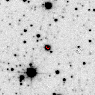
Figure 1: UKIDSS image of the X1908+075 region. North is up and east is left. The red circle indicates the Chandra position of the X-ray source. Size of the image: 1′$\times$ 1′.

Figure 2: H and K-Band spectra of the X1908+075 donor star.

3 Stellar atmosphere models

During the analysis, the observed spectra are compared with synthetic spectra calculated with the Potsdam model atmosphere code (PoWR). The PoWR code provides a model for a spherical symmetric star with an expanding atmosphere by iteratively solving the radiative transfer equation and the statistical equilibrium equations in non-LTE. The code further includes energy conservation and treats both the wind and photosphere in a consistent scheme.

The main aspects of the code are summarized in Gräfener et al. (2002) and Hamann & Gräfener (2003). This code has been applied to all kinds of stars that could be potential donors in wind-fed HMXB systems, such as O and B stars (e.g. Oskinova et al. 2011; Evans et al. 2012) and Wolf-Rayet (WR) stars (e.g. Hamann et al. 2006; Sander et al. 2012). Wind inhomogeneities are considered in a so-called “micro-clumping” approach, assuming that the wind is not smooth, but instead consisting of optical thin cells with an increased density and a void interclump medium (cf. Hamann & Koesterke 1998).

The “stellar radius” $R_{\ast}$ marks the lower boundary of the model atmosphere and is set at a Rosseland optical depth of $\tau=20$, where we assume that the hydrostatic equation is fulfilled. In the quasi-hydrostatic regime we use this equation to calculate a hydrodynamically-consistent velocity field(Sander et al. 2015). In the outer part we assume a so-called “beta-law’,’

$$\varv(r)=\varv_{\infty}\left(1-\frac{R_{\ast}}{r}\right)^{\beta},$$ (1)

with $\varv_{\infty}$ being the terminal velocity of the wind from the donor star. Both parts are connected such that a smooth transition is guaranteed. That means not only the velocities but their gradients are equal at the connection point, which is usually close to the sonic point where the wind velocity is equal to the speed of sound. In the final model for the donor star of X1908+075, we adopted an exponent of $\beta=1.2$, after testing models with different $\beta$ values. Models with lower values of $\beta$ down to $0.6$ lead to slightly lower fit qualities. The precise choice of beta has hardly any effect on the obtained parameters, for instance, for the estimated mass-loss rate: reducing $\beta$ by $0.2$ requires approximately an increase of $0.05\,$dex in $\dot{M}$ to still reproduce the observed strength of the Br$\gamma$ line.

With a given luminosity $L$, the stellar temperature $T_{\ast}$ can be obtained from $L$ and $R_{\ast}$ via the Stefan-Boltzmann relation. Apart from $L$, $T_{\ast}$, and $\varv_{\infty}$, the other main model parameters are the effective surface gravity $g_{\text{eff}}$ and the wind mass-loss rate $\dot{M}$. The $\log g_{\mathrm{eff}}$ corrects for full radiation pressure $a_{\text{rad}}$, i.e. it considers not only Thomson scattering, but also the non-negligible continuum and line accelerations. While the actual calculation for the model stratification is depth dependent, we use a mean value of $\Gamma_{\text{rad}}:=a_{\text{rad}}/g$ to define an output value for $g_{\text{eff}}$ that is related to the pure gravitational acceleration via

$$\log g_{\text{eff}}=\log g+\log\left(1-\overline{\Gamma}_{\text{rad}}\right)\text{.}$$ (2)

The details are described in Sander et al. (2015). In addition, the clumping factor $D$ describes the maximum density contrast reached in the outer parts of the wind. In our models we assume that the density contrast starts around the sonic point and increases outwards until the specified value of $D$ is reached. For our O- and B-star models, we assume a solar composition according to Asplund et al. (2009), see Table 2. An overview of the model atoms used in the PoWR calculations is given in Table 3.

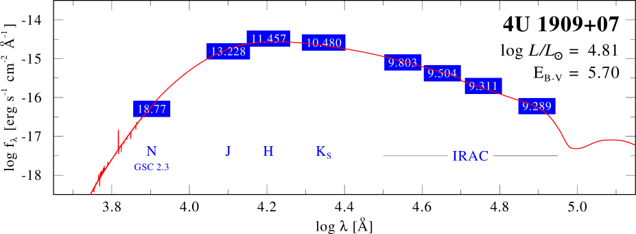
Figure 3: Spectral energy distribution (SED) of the 4U 1907+09 donor star. The PoWR model (red solid line) is reddened such that it fits the observed photometry marks (blue boxes).

4 Results

We simultaneously reproduce the normalized line spectrum and the spectral energy distribution (SED) of X1908+075 by our calculated PoWR model (see Fig. 3). The SED is compared to available photometry from IRAC (Spitzer Science 2009), 2MASS (Skrutskie et al. 2006) and Lasker et al. (2008). First, the interstellar reddening colour excess $E_{\text{B-V}}$ is determined. Then, we apply the reddening law by Fitzpatrick (1999) to calculate $E_{\text{J-K}}$ and compare this value with the estimated extinction curve in the direction towards X1908+075. This curve, shown in Fig. 4, was obtained following the procedure outlined in Cabrera-Lavers et al. (2007): red clump giants are selected over a near-infrared colour-magnitude diagram. Since this population has a well-calibrated luminosity function, we can compare their intrinsic and apparent colour and magnitude to derive both their distance along the line of sight and the reddening to which they are subjected. Once this ($d$, $E_{\text{J-K}}$)-curve is established, we can compare it with the colour excess of our source ($E_{\text{J-K}}=1.66$) to estimate a more accurate distance of 4.85 $\pm$ 0.50 kpc compared to the previous estimation by Morel & Grosdidier (2005).

Since the total luminosity $L$ is critically dependent on the distance, we can estimate the luminosity, using our SED fit, once we have determined the new distance of the system. We obtain a value of $10^{4.81}L_{\odot}$. This value is used in our atmosphere model. As we already need a model for the SED fit, the whole process was iterated until we obtained the consistent solution described above. The corresponding stellar radius $R_{\ast}=16\,R_{\sun}$ inferred from temperature and luminosity perfectly agrees with the radius deduced for a wind-fed system in Levine et al. (2004).

Prior to modelling the spectrum, we compared our data with the standard atlases of OB stars in the $H$ and $K$ bands (Hanson et al. 1998, 2005) to constrain the parameter space of the models. The He ii lines at 1.693 $\mu$m and 2.188 $\mu$m are weak or maybe even absent as it is hard to distinguish them from the noise here. Together with the relatively strong hydrogen absorption lines in the H-band, this points to a spectral type later than O9.5 (Hanson et al. 1996, 2005). The luminosity class is more difficult to ascertain. Several indicators point to a high luminosity: The He I series lines are narrow and the H series can be seen, at our resolution, up to Br 19. However, the equivalent width of the He I line at 1.700 $\mu$m ($\sim 1.9\AA$) is lower but comparable to that of the Brackett (11-4) line at 1.6814 $\mu$m (2.8 Å). This is typically seen in supergiants rather than in main-sequence stars where EW(HeI) $<$ EW(Br 11-4). All these properties suggest a high luminosity class. In addition, Br$\gamma$ in emission is a spectroscopic feature only observed in two objects within the sample analysed by Hanson et al. (2005). Both sources belong to the rare class of ON/BN supergiants.

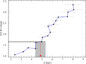
Figure 4: Estimated extinction curve from the direction of X1908+075, obtained following the procedure outlined in Cabrera-Lavers et al. (2007).

We calculate a set of stellar models starting with typical properties of O9.7-B4 stars. An iterative improvement of the parameters is performed until a sufficient fit of both, the spectral lines and the photometry, is achieved. Figure 5 shows the normalized line spectrum in the H and $\text{K}_{\text{S}}$ bands together with the best-fitting PoWR model. Most spectral features can be reproduced, apart from the observed asymmetric shape in some of the hydrogen absorption lines in the H band. The corresponding stellar parameters are compiled in Table 2. Because of the limited spectral range and the absence of unblended metal lines, there is a certain degeneracy in the spectral appearance that introduces a quite large error margin. The observation is best reproduced by a model with $T_{\ast}=23$ kK and $\log g_{\mathrm{eff}}=3.0$, which is in line with an early B-type donor. To constrain the temperature, we used the Bracket series as well as He i at 1.7 $\mu$m and He ii at 1.693 $\mu$m. The absence of He ii emission at 2.189 $\mu$m excludes temperatures higher than $\approx 30\,$kK. In the range between $21$ and $28\,$kK one can always find a model that reproduces Br$\gamma$ and a few other lines sufficiently, but most of them fail to predict the strength of the very sensitive He i 2.059 $\mu$m line. As the low terminal velocity deduced from Br$\gamma$ already favours the lower part of the deduced temperature range, we found that a model with $T_{\ast}=23$ kK best fits the observation.

For $\log g_{\mathrm{eff}}$, the right wings of the bracket series could be used to determine an upper limit and excluded values $\ga 3.3$. These stronger effective gravity values would lead to broader wings than observed, including an unobserved red absorption wing for Br$\gamma$.

To reproduce the shape of the observed line profiles, the emergent spectrum of the PoWR model was convolved with a rotational velocity of $100\,$km/s. Given the limited spectral quality this should be seen as just a rough approximation with a relatively large uncertainty of $\pm 50\,$km/s.

Before the donor was detected, Levine et al. (2004) speculated that the donor might be a WR star. With the first infrared spectra of the donor obtained by Morel & Grosdidier (2005) it became clear, that this is most likely not the case. Instead, Morel & Grosdidier (2005) claim that the donor star would be an O7.5-9.5If supergiant, based on the emission feature next to the He i absorption line at $2.11\,\mathrm{\mu m}$. This feature is actually a complex structure consisting of He i, N iii, C iii, and O iii emission lines. The C, N and O components are originated from high excitation states, and since not all of them are covered in our atomic database, this peak cannot be reproduced with the PoWR model. While one might argue that this line could be an indicator of enhanced nitrogen, this should also affect N iii $2.2471$/$2.2513\,\mathrm{\mu m}$. Since these lines are not detectable in the spectrum, we keep a solar chemical composition.

The Br$\gamma$ line is the only line in the observed spectra formed in the stellar wind. Therefore, the determination of the terminal wind velocity can only rely on fitting the wind broadening of this line. This fitting results in $\varv_{\infty}=500\pm 100$ km/s with a relatively large error margin. Significantly larger values would over predict the emission line width or even lead to additional absorption features that are not observed.

The precise B-subtype is hard to determine from the given observations. The relationship between the He I line at 1.700 $\mu$m and the Brackett (11-4) line at 1.6814 $\mu$m (the former being deeper than the latter) clearly shows that the donor should be B0.5 or even B0 (Fig. 2 in Hanson et al. 1998). The obtained temperature of $23\,$kK, however, favours a slightly later subtype around B2. We therefore specify the spectral type of the X1908+075 donor star to be in the range between B0 to B3.

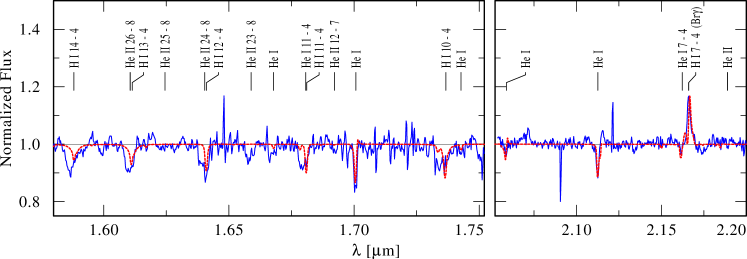
Figure 5: The observed spectrum (thin blue line) – $H$ band (left panel), $K$ band (right panel) – is compared with the best-fitting PoWR model (red thick dotted line). Noticeable spectral lines are identified.

Table 2: Derived properties of the X1908+075 donor star.

Parameter	Obtained value
$T_{\ast}$	$23.0^{+6}_{-3}\,$kK
$T_{\frac{2}{3}}$	$22.7^{+6}_{-3}\,$kK
$\log L/L_{\odot}$	$4.81\pm 0.25$
$E_{\text{B-V}}$	$5.7\pm 0.1$
$d$	$4.85\pm 0.50$ kpc
$\varv_{\infty}$	$500\pm 100$ km/s
$R_{\ast}$	$16\,R_{\odot}$
$\log g_{\text{eff}}$	$3.0\pm 0.2$
$\log g$	$3.2\pm 0.2$
$M_{\text{spec}}$	$15\pm 6$ $M_{\odot}$
$\dot{M}$	$10^{-6.55}$ $M_{\odot}/$yr
$D$	$10$
$\varv_{\text{dop}}$	$20$ km/s
$\varv_{\text{rot}}$	$100\pm 50$ km/s
$M_{\text{V}}$	$-5.29$
$X_{\text{H}}$	$0.735$
$X_{\text{He}}$	$0.256$
$X_{\text{C}}$	$2.2\cdot 10^{-3}$
$X_{\text{N}}$	$6.1\cdot 10^{-4}$
$X_{\text{O}}$	$5.3\cdot 10^{-3}$
$X_{\text{Fe}}$	$1.1\cdot 10^{-3}$
$\log Q_{0}$	$47.1\,$s-1

Table 3: Overview of the used model atoms.

Ion	Levels	Lines
H i	22	595
H ii	1	325
He i	35	0
He ii	26	231
He iii	1	0
C i	2	0
C ii	32	703
C iii	40	630
C iv	21	703
C v	1	1
N i	1	1
N ii	38	496
N iii	36	780
N iv	38	210
N v	2	0
O i	2	1
O ii	36	630
O iii	33	528
O iv	25	300
O v	2	1
Fe i	1	0
Fe ii	2	1
Fe iii	8	25
Fe iv	11	49
Fe v	13	69
Fe vi	17	121
Fe vii	11	52
Fe viii	1	0

5 Discussion

5.1 On the accretion scenario

We are going to demonstrate that the wind mass-loss rate derived in our model is compatible with the observed average X-ray luminosity, considering a Bondi-Hoyle-Lyttleton (BHL) accretion scenario (Bondi & Hoyle 1944, and references therein). We estimated the fraction of the wind that is gravitationally captured by the compact object to estimate the accretion luminosity. First, we determine the orbital separation of the neutron star to the donor star ($a$). Given our spectroscopic mass, the orbital period derived by Levine et al. (2004) (see Table 1) and assuming a canonical neutron star of 1.4M_⊙, we obtain $a=(1.98\pm 0.10)\times 10^{12}$ cm. Second, we determine the Bondi-Hoyle accretion radius, and finally, we estimate the captured fraction of the wind as follows:

$$f(a)=\frac{\dot{M}_{\mathrm{captured}}}{\dot{M}_{\mathrm{wind}}}=\frac{r_{\mathrm{accr}}^{2}}{4a^{2}}\\ \mathrm{;}\\ r_{\mathrm{accr}}=\frac{2GM_{\mathrm{NS}}}{\varv(a)_{\mathrm{wind}}^{2}+\varv(a)_{\mathrm{orb}}^{2}}.$$ (3)

Therefore, the captured fraction of the wind depends on the wind velocity and the orbital velocity as a function of the orbital separation. From our model we obtain a $\varv_{\mathrm{wind}}=190\pm 40\;\mathrm{km/s}$ for the given $a$, and we estimate an orbital velocity of $\varv_{\mathrm{orb}}=330\pm 20\;\mathrm{km/s}$ (considering our spectroscopic mass, a canonical neutron star of 1.4M_⊙ and the obtained $a$), which leads to a captured fraction of the wind of $f(a)=0.0044\pm 0.0016$.

Once we know the captured fraction of the wind, we can estimate the X-ray luminosity generated by the accretion of this fraction of the wind onto the neutron star as follows:

$$L_{\mathrm{accr}}=\frac{GM_{\mathrm{NS}}\dot{M}_{\mathrm{captured}}}{R_{\mathrm{NS}}}\xi=\frac{GM_{\mathrm{NS}}f(a)\dot{M}_{\mathrm{wind}}}{R_{\mathrm{NS}}}\xi,$$ (4)

where $\xi$ is the efficiency factor of energy conversion and $R_{\mathrm{NS}}=15\mathrm{km}$, obtaining a $L_{\mathrm{accr}}=[(10\pm 3)\times 10^{36}]\;\xi\;\mathrm{erg/s}$.

However, we know that the source is persistent in X-rays with an X-ray luminosity of $\sim(1-4)\times 10^{36}\;\mathrm{erg/s}$ in the $2-30$ keV band according to Levine et al. (2004) and using our distance value. Since we expect significant X-ray emission below 2 keV, we estimate the X-ray luminosity in the 0.1–50 keV energy range assuming the spectral model used by Levine et al. (2004), obtaining $L_{\mathrm{X}}=(1.4-5.6)\times 10^{36}\;\mathrm{erg/s}$. Taking an average value of $L_{\mathrm{X}}=3.5\times 10^{36}\mathrm{erg/s,}$ we obtain an energy conversion efficiency of $0.36\pm 0.13$, which is a reasonable value for a wind-fed system.

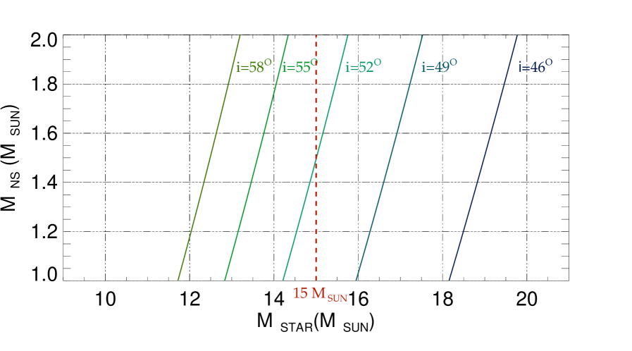
Figure 6: Relations between the donor mass and neutron star mass. Lines of constant orbital inclination constructed from the mass function of Levine et al. (2004) are labelled. The X-axis range corresponds to the spectroscopic mass error margin, while the Y-axis range covers the range permitted for a neutron star mass (e.g. Lattimer 2012).

5.2 On the wind mass-loss rate determination

Our stellar atmosphere model is used to derive a wind mass-loss rate $\dot{M}_{\text{PoWR}}=2.8\times 10^{-7}\,M_{\odot}/$yr, significantly lower than the value of $\gtrsim$ $4\times 10^{-6}$ M_⊙ yr^-1 derived from X-rays by Levine et al. (2004). Levine et al. (2004) employed the density stratification of the wind expected from a $\beta$-law of the velocity field and the continuity equation. Using the orbital parameters that they derived, they make a fit of the orbital modulation of the X-rays absorption ($N_{\mathrm{H}}$ ). From this fit it is possible to derive $\dot{M}/\varv_{\infty}$, so an assumption about $\varv_{\infty}$ is required to make an estimation of $\dot{M}$. Since our adopted $\varv_{\infty}$ is very low, it is very likely that Levine et al. (2004) assumed a higher value of $\varv_{\infty}$. Therefore, their estimations of $\dot{M}$ must be corrected by a factor $F=500/\varv_{\infty}^{\text{Levine}}$. Even using this correction, it is clear that the estimations from the orbital modulation of the $N_{\mathrm{H}}$ yield higher values of $\dot{M}$ than the values obtained in this work. We have used a clumping factor $D=10$. Decreasing $D$ in order to increase $\dot{M}$, worsens the quality of the fit. For instance, a more modest value of clumping $D=4$ (see Appendix A, in which models with different D values are compared), yields a higher mass-loss rate $\dot{M}=4.6\cdot 10^{-7}\,M_{\odot}/$yr. In summary, there is a discrepancy between the X-rays estimation by Levine et al. (2004) and our model estimation ($\dot{M}_{\text{PoWR}}$). The plausible reasons are: a density enhancement in the vicinity of the neutron star that systematically increases the measured $N_{\mathrm{H}}$ ; and/or an accumulation of uncertainties in both methods, including $\dot{M}$, $D$ for the stellar atmosphere calculations, and $\varv_{\infty}^{\text{Levine}}$, $N_{\mathrm{H}}$ and its variability in X-rays.

In addition to the comparison with the mass-loss rate estimation from X-rays, we can compare our estimation to the predictions by Vink et al. (2000) for OB stars. These predictions distinguish two regimes depending on the effective temperature of the star (the so-called bi-stability jump). These two regimes are also characterized by a different ratio $r=\varv_{\infty}/\varv_{\text{esc}}$, where $\varv_{\text{esc}}$ is the escape velocity (corrected for the radiative acceleration due to Thomson scattering). In the hot regime the effective temperature is over $30$ kK and $r\sim 2.6$, whereas in the cool regime the effective temperature lies below $22.5$ kK and $r\sim 1.3$. Hence, given our parameters (see Table 2), and $\varv_{\text{esc}}=560$ km/s, the donor star in X1908+075 belongs to the cool regime. Vink et al. (2000) gives an estimation of the mass-loss rate depending on the luminosity, the mass, the ratio $r,$ and the effective temperature of the star. Plugging our parameters into the cool regime equation, we find $\dot{M}_{\text{Vink}}\simeq 8\times 10^{-7}\,M_{\odot}/$yr. The difference between our $\dot{M}_{\text{PoWR}}$ and the expected $\dot{M}_{\text{Vink}}$ is on the order of $\sqrt{D}$, hinting that a porous wind treatment in the mass-loss predictions might possibly solve this discrepancy.

5.3 Enclosing the inclination angle of the system

We can also constrain the inclination of the system using our spectroscopic mass ($15\pm 6$ $M_{\odot}$) and the mass function given by Levine et al. (2004). Figure 6 shows lines of constant orbital inclination for the allowed spectroscopic mass range and the permitted neutron star mass range by the equation of nuclear state (e.g. Lattimer 2012). The allowed inclination values are in the range 46^∘ $<$ i $<$ 58^∘. The canonical neutron star mass of 1.4 M_⊙ favours an inclination of $\sim$ 50^∘. Our determination agrees with the estimation of Levine et al. (2004), who used a completely independent method and obtained the inclination from the orbital modulation of N_H.

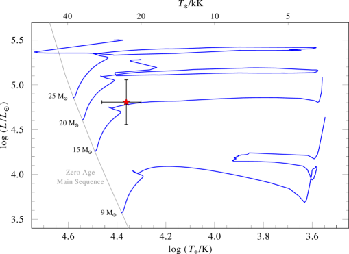
Figure 7: Evolutionary tracks using the Geneva Stellar Models (Ekström et al. 2012) for solar metallicity and a rotation rate of $\varv_{\mathrm{ini}}/\varv_{\mathrm{crit}}=0.4$ on ZAMS (it corresponds to 170 km/s for an initial mass of 20$M_{\odot}$). Initial masses are: 9, 15, 20, and 25$M_{\odot}$. The position of X1908+075 is marked by the red star.

5.4 On the evolutionary phase

Our spectrum shows Br$\gamma$ in emission (see Sect. 4), which indicates that the source could belong to the rare class of ON/BN supergiant systems. There are several observational hints that point to this classification:

• This class of objects commonly show variability (e.g. Walborn 1976). Comparing our data set with Morel & Grosdidier (2005) reveals that Br$\gamma$ for X1908+075 is not only in emission, but varies significantly between the two observations. We measured an equivalent width for this line to be -4.3 Å (55018.97 MJD), which differs by a factor of  3 compared to the value of -1.4 Å (52418.54 MJD) found by Morel & Grosdidier (2005). The peak height in the normalized spectrum is also about three times higher than in the observation discussed in Morel & Grosdidier (2005).

• ON/BN supergiant systems seem to be nitrogen enriched (e.g. Corti et al. 2009). X1908+075 has likely gone through a common envelope phase in the past because of the proximity of the neutron star and its companion ($R_{\text{orb}}\approx 1.7R_{\ast}$). Consequently, the source could be nitrogen enriched (e.g. Langer 2012) and thus, show spectral features similar to ON/BN stars as seen in Hanson et al. (2005). However, our spectrum does not show unblended metal lines, which makes it hard to determine the CNO abundances. Models with increased nitrogen did not improve the fit and thus we cannot confirm if the star is really nitrogen enriched or not.

• ON/BN supergiant systems are candidates for interacting binaries (e.g. Walborn 1976). The projected rotational velocity derived from our data is high compared to that of isolated OB stars (Simón-Díaz & Herrero 2014). This could be the result of a tight binary interaction of the system in the past.

• Figure 7 shows the evolutionary tracks using the Geneva Stellar Models (Ekström et al. 2012) computed for single-star evolution and initial masses of $9$, $15$, $20$, and $25\,M_{\odot}$. Thus, assuming that binary interactions in our system have been negligible in the past, we can compare the current position of our donor star to these tracks. Indeed, the position of X1908+075 in the HR diagram is very close to the $15\,M_{\odot}$-track in coincidence with our spectroscopic mass. However, as previously discussed, there are several indications that point towards a former interaction that would make the star to appear much younger than an isolated star (Langer 2012). Nevertheless, we can neither confirm nor rule out this expected rejuvenation of the system due to the large uncertainties in our spectroscopic mass and effective temperature.

5.5 On the asymmetry of some of the hydrogen absorption lines

The hydrogen absorption lines of our data show an additional component with respect to the model (see Fig, 5). These additional absorptions have a measured blueshift of about 200 km/s compared to the rest of the spectrum. The additional absorption is comparable to the intensity of the lines in the model. This effect is only seen in the hydrogen absorption lines, while the helium absorption lines and Br$\gamma$ are perfectly reproduced by our model atmosphere.

A first hypothesis would be that these lines might be shifted because of the tidal disruption expected in this kind of close binary systems (Abubekerov et al. 2004) in which the optical companion is pear-shaped, leading to a non-uniform temperature distribution in the atmosphere of the star. Even though we cannot completely rule out this hypothesis since PoWR assumes a spherically symmetric wind, it is certainly quite unlikely since there is no reason why this effect is only seen in the hydrogen absorption lines.

Another hypothesis is that these additional absorptions are due to the presence of a density enhancement caused by the interaction with the neutron star, as seen in the simulations of Blondin et al. (1991) and Manousakis et al. (2012). This hypothesis is supported by the fact that these blueward shifts of the absorption features are only seen in the H-band spectrum, while the lines in the K-band spectrum are perfectly reproduced. Both spectra were taken at different orbital phases. The H-band spectrum was taken at orbital phase $\phi=0.158$, with the neutron star travelling to quadrature where the projected orbital velocity towards the observer is maximum. For an orbital speed of $\varv_{\mathrm{orb}}=330\leavevmode\nobreak\ \mathrm{km/s}$ and an orbital inclination of the order of $i\approx 50^{\rm o}$ this component would be $\varv_{\mathrm{orb}}\sin i=252\leavevmode\nobreak\ \mathrm{km/s}$, of the same order than the measured blueshift. Moreover, the K-band spectrum was taken during orbital phase $\phi=0.374$ with the neutron star approaching inferior conjunction where the projected orbital velocity towards the observer is zero. As a consequence, the K-band spectrum does not show this effect.

To reproduce the additional absorptions, however, we need the column density of the extra absorber to be at least equal to the column density from the photosphere to the observer, which is $\sim 1\leavevmode\nobreak\ \mathrm{g\,cm^{-2}}$ in our model, corresponding to $N_{\text{H}}\leavevmode\nobreak\ \sim\leavevmode\nobreak\ 60\leavevmode\nobreak\ \times\leavevmode\nobreak\ \mathrm{10^{22}at\,cm^{-2}}$. Moreover, this extra absorber has to be hot enough to produce a significant amount of hydrogen lines at level 4. Manousakis et al. (2012) simulations corresponding to our mass-loss rate and terminal velocity has shown a very modest density enhancement in the vicinity of the neutron star in comparison to our required estimations. Furthermore, Levine et al. (2004) were able to explain the observed $N_{\text{H}}$ orbital modulation appealing to the wind without any further structure. Therefore, it is quite unlikely that the observed extra absorption is due to the presence of a density enhancement produced by the interaction of the neutron star with the stellar wind.

6 Conclusions

For the first time, we obtained a reliable set of stellar and wind parameters for the donor star in the high-mass X-ray binary X1908+075, allowing us to determine various parameters of the system. Most of our results are in line with what is expected from a wind-fed binary system. The main conclusions of this work are:

• The donor star of X1908+075 is identified with an early B-type star (B0-B3). Its main parameters are: $M_{\mathrm{spec}}$ = $15\pm 6$ $M_{\odot}$, $T_{\ast}=23_{-3}^{+6}\,$kK, $\log g_{\mathrm{eff}}=3.0\pm 0.2$, and $\log L/L_{\odot}$ = $4.81\pm 0.25$.

• The low effective gravity perfectly fits with a supergiant star, favouring this classification. Moreover, the presence of Br$\gamma$ in emission could indicate that the source belongs to the rare class of nitrogen-enriched B-type supergiant stars.

• The source shows a variable stellar wind, since the equivalent width of Br$\gamma$ emission line in our K-spectrum is three times higher than the value found by Morel & Grosdidier (2005).

• The derived parameters along this work are consistent with a wind-fed high-mass X-ray binary within the Bondi-Hoyle-Lyttleton (BHL) accretion scenario.

• The distance to the system is constrained to the value of 4.85 $\pm$ 0.50 kpc, which is well inside the previously estimated range of 7 $\pm$ 3 kpc reported by Morel & Grosdidier (2005).

• The wind mass-loss rate we have obtained from the spectral fit is one order of magnitude lower than the Levine et al. (2004) estimation using X-ray observations.

• The inclination of the system is constrained, favouring an inclination $\sim$ 50^∘, assuming a canonical 1.4 M_⊙ neutron star.

As a general conclusion, we would like to emphasize that to understand wind-fed binary systems in a coherent way, one needs to analyse the donor stars with stellar atmosphere models to constrain their parameters and to understand how the wind of the donor star interacts with its compact companion.

Appendix A On the clumping factor and mass-loss rate dependency

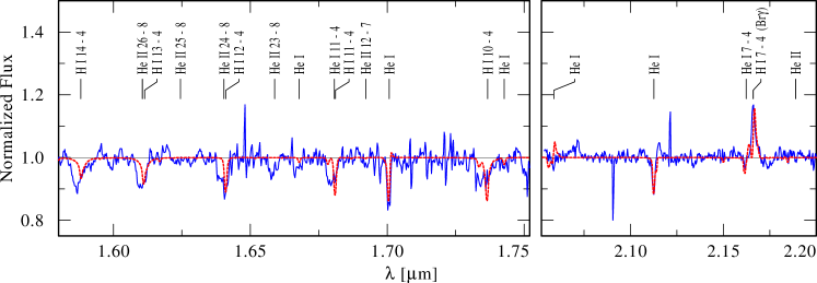
Figure 8: The observed spectrum (thin blue line) – $H$ band (left panel), $K$ band (right panel) – is compared with the best-fitting PoWR model (dotted line) for different D factors: D=10 (top panel); D=4 (middle panel); D=1 (low panel).