Capture Dynamics of Ultracold Atoms in the Presence of an Impurity Ion

Abstract

We explore the quantum dynamics of a one-dimensional trapped ultracold ensemble of bosonic atoms triggered by the sudden creation of a single ion. The numerical simulations are performed by means of the ab initio multiconfiguration time-dependent Hartree method for bosons which takes into account all correlations. The dynamics is analyzed via a cluster expansion approach, adapted to bosonic systems of fixed particle number, which provides a comprehensive understanding of the occurring many-body processes. After a transient during which the atomic ensemble separates into fractions which are unbound and bound with respect to the ion, we observe an oscillation in the atomic density which we attribute to the additional length and energy scale induced by the attractive long-range atom-ion interaction. This oscillation is shown to be the main source of spatial coherence and population transfer between the bound and the unbound atomic fraction. Moreover, the dynamics exhibits collapse and revival behavior caused by the dynamical build-up of two-particle correlations demonstrating that a beyond mean-field description is indispensable.

I Introduction

The theoretical description of degenerate atomic quantum gases has advanced significantly in the past two decades. It relies particularly on the separation of length scales of the external trapping potential, the inter-particle distances and the range of atomic interactions. In the ultracold regime, this allows to approximate the interaction by a contact potential (or simply pseudopotential) Huang and Yang (1957), which has proven tremendously powerful when applied to bosonic gases. The latter holds especially for the mean-field approximation leading to the well-known Gross-Pitaevsikii (GP) equation Gross (1963); Pitaevskii (1961) which describes the condensed state of a weakly interacting bosonic gas yielding a variety of phenomena such as collective excitations, solitons, and vortices Pitaevskii and Stringari (2003); Pethick and Smith (2008). For state-of-the-art methods, such as the density-matrix renormalization group Schollwöck (2011) and the multiconfiguration time-dependent Hartree method for bosons (MCTDHB) Alon et al. (2008) as well as its multi-layer extension (ML-MCTDHB) Cao et al. (2013); Krönke et al. (2013), the pseudopotential represents an essential simplification for the quantum dynamical description of many-boson systems in order to investigate the physics beyond the mean-field approximation. Even though the short-range interaction has proven to lead to exotic states of quantum matter like supersolidity Büchler and Blatter (2003) or crystalline phases Büchler (2011) and therefore represents an important case, not all ultracold atomic systems exhibit these short-range interactions. An example for the latter are chromium atoms which possess long-range magnetic dipolar interactions Stuhler et al. (2005); Lahaye et al. (2009).

Hybrid atom-ion systems represent a specific class of systems with a new scale of interactions due to the interplay between the charge of an ion and the induced dipole moment of a neutral atom Seaton and Steenman-Clark (1977). They have recently become available experimentally Smith et al. (2005); Zipkes et al. (2010); Schmid et al. (2010); Härter et al. (2012) and attracted increasing interest. Most of the current experiments, however, are based on the Paul trap scheme, whose drawback is the so-called micromotion which so far prevents from reaching the ultracold regime as shown in theoretical classical and quantum analyses Cetina et al. (2012); Krych and Idziaszek (2015). Corresponding studies showed that a large ion-atom mass ratio might help circumventing this limitation Cetina et al. (2012); Joger et al. (2014); Krych and Idziaszek (2015), although it is not yet clear whether the s-wave regime can be reached. Still, a recent detailed study has shown that specifically for the atom-ion pair $\mathrm{Li}$-$\mathrm{Yb}^{+}$ the ultracold regime can be reached experimentally Tomza et al. (2015). Given these findings, it is desirable to extend the theoretical understanding of ultracold neutral quantum many-body systems by the presence of ions. This attractive interaction induces, additional to the confinement, a further length and energy scale and it is therefore expected to lead to intriguing effects such as the formation of molecular ions Côté et al. (2002) and ion-induced density bubbles in the atomic cloud Goold et al. (2010). Apart from this fundamental point of view, these hybrid systems show versatile applications in quantum information processing as, for example, the controlled creation of entanglement Joger et al. (2014); Gerritsma et al. (2012), the realization of quantum gates Doerk et al. (2010), and the simulations of solid-state systems Bissbort et al. (2013).

In a previous study, we have investigated in detail the ground-state properties of an atom-ion hybrid system, consisting of a single static ion in the center of a bosonic atomic cloud. The dependence of relevant observables on the atom number and the interaction strength has been analyzed and we showed that the presence of an ion strongly affects them Schurer et al. (2014). For weakly interacting atoms, we found that the ion impedes the transition to the Thomas-Fermi regime while for strong atom-atom interaction it modifies the fragmentation behavior depending on the atom number parity. In the present work, we explore the impact of the second length and energy scale generated by the atom-ion interaction onto the dynamics of the atomic cloud. In particular, we envision the scenario in which we create a single ionic impurity in an ensemble of $N$ interacting atomic bosons. If the atomic cloud, initially prepared in the ground state of a harmonic trap, and the ion are suddenly brought into contact, this process resembles, to some extent, the sudden ionization of a single impurity atom within the atomic cloud. Here, however, we still neglect the ionic motion which is justified in case the ion is tightly trapped. We will see in the following that the second length and energy scale induces a coherent oscillation between states bound in the atom-ion potential and states of the harmonic trap. This oscillation occurs in addition to the usual harmonic excitation and reveals a collapse and revival behavior caused by the dynamical build-up of correlations.

This work is organized as follows. In Sec. II, we define the setup and explain the model of our hybrid atom-ion system. In addition, we introduce a cluster-expansion scheme which enables us to distinguish the single-particle dominated physics from the processes induced by the build-up of (quantum) correlations. In Sec. III, we explore the dynamical evolution of the hybrid system and identify the most important excited modes by means of our cluster-expansion approach. Sec. IV contains a brief convergence analysis which shows the necessity to use an advanced method like MCTDHB. Finally, we summarize our findings in Sec. V together with the conclusions and an outlook on future investigations.

II Model and Theoretical Approach

In the following, we introduce our model and define the process to initiate the dynamics. Further, we briefly outline the MCTDHB used for the simulations, define important quantities for the analysis, and introduce our cluster expansion approach which we exploit in order to analyze the many-body wave function.

II.1 Model of the System

We consider $N$ interacting bosonic atoms in a one-dimensional (1D) harmonic trap at zero temperature initially prepared in the ground state of the system which we compute by imaginary time propagation Kosloff and Tal-Ezer (1986) of an initial guess wave function. The short-range intra-atomic interaction is modeled by a contact pseudopotential. Into this atomic cloud, we immerse a single trapped impurity atom which does not interact with the other atoms. This could be achieved by tuning the inter-atomic interaction to zero by exploiting a Feshbach resonance Chin et al. (2010). At time $t_{0}=0$ this impurity atom is ionized by a laser pulse such that a single ion is created within the atomic cloud. The ionizing laser pulse is assumed to be far detuned from any possible resonance of the atomic cloud. Moreover, we assume pulse durations such that the ionization process takes place on much faster time scales than any possible response of the atomic cloud. This allows us to treat the ionization as an effectively instantaneous process. If the atomic impurity is trapped in a sufficiently deep and tight trap, the proposed scenario can be indeed achieved experimentally, as recently reported for optical trapping of a single ion Huber et al. (2014). Thus, at time $t_{0}=0$, the ion is assumed to be statically trapped at $z_{\mathrm{I}}=0$ in the atomic cloud. The motional excitations following this ionization process result in a rich dynamics which we analyze in Sec. III.

The interaction between the ion at $z_{\mathrm{I}}$ and an atom at $z_{\mathrm{A}}$ behaves in 1D at large distances as $-\alpha e^{2}/(2(z_{\mathrm{A}}-z_{\mathrm{I}})^{4})$ up to a minimal cutoff distance $R_{\mathrm{1D}}$ Idziaszek et al. (2007), where $\alpha$ is the polarizability of the atoms and $e$ the elementary charge. For numerical many-body simulations with MCTDHB it is more convenient, however, to define a model potential as Schurer et al. (2014):

$$V_{\mathrm{mod}}(z)=\mathrm{v}_{0}e^{-\gamma z^{2}}-\frac{1}{z^{4}+1/\omega}.$$ (1)

Here $z$ denotes the relative coordinate $z_{\mathrm{A}}-z_{\mathrm{I}}$. The model parameters $\mathrm{v}_{0}$,$\gamma$, and $\omega$ are determined by the short-range quantum defect parameters. The above potential asymptotically approach the $-1/z^{4}$ behavior at large distances, whereas at short distances it has a barrier which is designed such that the quantum defect theory results for the atom-ion scattering Idziaszek et al. (2009) can be reproduced. Additionally to the harmonic confinement, this interaction introduces a second length $R^{*}=\sqrt{\alpha e^{2}m/\hbar^{2}}$ and energy scale $E^{*}=\hbar^{2}/(2m{R^{*}}^{2})$ to the system, where $m$ is the mass of a single neutral atom.

In summary, the system can be described by the following many-body Hamiltonian (in $E^{*}$ and $R^{*}$ units)

$$\hat{H}= \sum_{i=1}^{N}\underbrace{\left[-\frac{\partial^{2}}{\partial z_{i}^{2}}+\frac{1}{l^{4}}z_{i}^{2}+\theta(t-t_{0})V_{\mathrm{mod}}(z_{i})\right]}_{\hat{h}_{i}}$$

$$+g\sum_{i<j}^{N}\delta(z_{i}-z_{j})$$ (2)

with the harmonic trap of frequency $\omega_{0}$ and characteristic length $l=\sqrt{\hbar/(m\omega_{0})}/R^{*}$, and the intra-atomic contact interaction strength $g$. The ionic part is switched on at time $t_{0}$ by a step-function $\theta(t-t_{0})$. Thereby, we term the Hamiltonian of a single boson as $\hat{h}_{i}$. In the following, we denote the stationary eigenenergies of $\hat{h}_{i}(t>t_{0})$ for fixed $t$ with $\epsilon_{j}$ and the corresponding single-particle eigenstates with $\phi^{0}_{j}(z_{i})$ such that $\hat{h}_{i}(t>t_{0})\phi^{0}_{j}(z_{i})=\epsilon_{j}\phi^{0}_{j}(z_{i})$. Hereafter, for the sake of numerical convenience, we set $l=0.5R^{*}$, which would corresponds to $\omega_{0}=2\pi\cdot 3.3\,\mathrm{k}\mathrm{Hz}$ and $l=188\,\mathrm{n}\mathrm{m}$ for ⁸⁷Rb atoms. We will see that this choice does not affect qualitatively the observed dynamics. Furthermore, we choose a weak intra-atomic interaction strength $g=2E^{*}R^{*}$ and small atomic ensembles consisting of $N=2$ up to $N=10$ neutral atoms. Besides, we fix the model parameters to $\omega=80(R^{*})^{-4}$, $\mathrm{v}_{0}=3\omega$ and $\gamma=4\sqrt{10\omega}$. We refer here to Ref. Schurer et al. (2014) for a detailed discussion of the chosen parameters as well as for the experimental conditions needed for the quasi-1D regime. Our above choice leads to two bound states for the atoms in the atom-ion potential which are localized on both sides of the ion but vanish at $z_{\mathrm{I}}$. Even though we neglect the motion of the ion, we term the two states below $E=0$ bound states while we refer to the remaining states as trap states (with $E>\hbar\omega_{0}/2$). In Fig. 1, we show the total potential for the atoms together with the energies $\epsilon_{j}$ as well as the lowest single-particle state $\phi^{0}_{1}(z)$, bound in the atom-ion potential, and the state $\phi^{0}_{5}(z)$. The arrows indicate the possible processes that can occur: within the trap (green arrow), in the atom-ion potential (white arrow), and between those two scales (oblique magenta arrows).

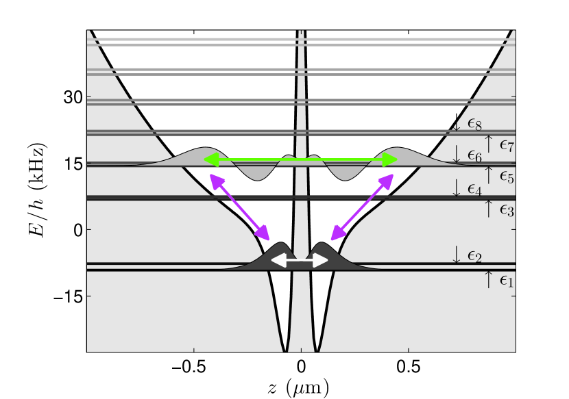
Figure 1: The effective potential (gray shaded area in background) consisting of the harmonic trap and the atom-ion interaction potential for the ${}^{87}\mathrm{Rb}$ atom. Further, we show the single-particle energy levels $\epsilon_{j}$ indicated by straight horizontal lines. In addition, the energetically lowest single-particle state $\phi^{0}_{1}(z)$ (dark gray area) and the trap state $\phi^{0}_{5}(z)$ (light gray area) are sketched with arbitrary but equal scaling. Possible types of dynamics occurring in the system are indicated by arrows.

II.2 Theoretical Approach

We explore the quantum dynamics of the many-body system described by the wave function $|\Psi\rangle$ by means of the numerically exact ab initio method MCTDHB. Its main idea is that by using $m$ time-dependent variationally optimized single-particle basis functions, the number of basis functions can be kept rather small. More precisely, the many-body wave function $|\Psi\rangle$ for $N$ bosons is expanded in bosonic number states $|{\mathbf{n}}(t)\rangle$

$$|\Psi(t)\rangle=\sum_{{\mathbf{n}}|N}A_{{\mathbf{n}}}(t)|{\mathbf{n}}(t)\rangle$$ (3)

in order to take into account the indistinguishability of the bosons. Note that in a number state $|{\mathbf{n}}(t)\rangle$, each boson occupies one of the $m$ time-dependent single-particle functions (SPFs) $|\Psi_{j}(t)\rangle$ and that the vector ${\mathbf{n}}=(n_{1},\cdots,n_{m})$ contains the occupation numbers $n_{j}$ of every SPF. Besides, the sum in Eq. (3) goes over all possible ${\mathbf{n}}$ with $\sum_{j}n_{j}=N$, which is denoted by the symbol ${\mathbf{n}}|N$. With this ansatz for the many-body wave function, the temporal evolution of the wave function $|\Psi(t)\rangle$ is obtained by means of the Dirac-Frenkel variational principle Dirac (1930); Frenkel (1934) which guarantees a variational optimal many-body solution. We would like to emphasize that not only the coefficients $A_{{\mathbf{n}}}(t)$ but also the SPFs $|\Psi_{j}(t)\rangle$ are adapted in time to the many-body dynamics in order to allow for the largest possible overlap between the ansatz (3) and the true many-body wave function. We refer for a detailed description of the method to Refs. Alon et al. (2008); Cao et al. (2013); Krönke et al. (2013).

The analysis of the full many-body wave function $|\Psi\rangle$ is generally a complicated task due to the underlying high dimensionality resulting from the $N$ degrees of freedom. In order to analyze the time-dependent many-body wave function in detail, we inspect two different quantities: The one- and two-particle reduced density matrices which allow for the investigation of spatial coherence and correlations Sakmann et al. (2008), and clusters enabling us to analyze coherence and correlations in terms of any single-particle basis. We transfer and adapt the notion of clusters from Ref. Kira and Koch (2006) to bosonic systems of few particles.

II.2.1 Density Matrices

The reduced one- and two-particle density matrices are defined via the expectation values of the field operators $\hat{\Psi}^{\dagger}{\left(x\right)}$ and $\hat{\Psi}^{{\color[rgb]{1,1,1}\dagger}}{\left(x\right)}$ as $\rho_{1}(x,y,t)=\langle\hat{\Psi}^{\dagger}{\left(x,t\right)}\hat{\Psi}^{{\color[rgb]{1,1,1}\dagger}}{\left(y,t\right)}\rangle$ and $\rho_{2}(x,y,y^{\prime},x^{\prime},t)=\langle\hat{\Psi}^{\dagger}{\left(x,t\right)}\hat{\Psi}^{\dagger}{\left(y,t\right)}\hat{\Psi}^{{\color[rgb]{1,1,1}\dagger}}{\left(y^{\prime},t\right)}\hat{\Psi}^{{\color[rgb]{1,1,1}\dagger}}{\left(x^{\prime},t\right)}\rangle$, respectively. Their spectral decomposition can be written in terms of the natural populations $\lambda_{j}(t)$ and the natural orbitals $\Phi_{j}(x,t)$

$$\rho(x,x^{\prime},t)=\sum_{j}\lambda_{j}(t)\Phi_{j}^{*}(x,t)\Phi_{j}(x^{\prime},t),$$ (4)

and the natural populations $\gamma_{j}(t)$ and natural geminals $\Phi_{j}(x,x^{\prime},t)$

$$\rho_{2}(x,y,y^{\prime},x^{\prime},t)=\sum_{j}\gamma_{j}(t)\Phi_{j}^{*}(x,y,t)\Phi_{j}(x^{\prime},y^{\prime},t),$$ (5)

respectively. This natural representation of the reduced density matrices has several advantages. For example, the natural populations can be used to identify the degree of fragmentation of the system Penrose and Onsager (1956) and to judge the convergence of our numerical simulations Beck et al. (2000). Further, the natural orbitals build always a very suitable single-particle basis set for the description of the dynamical system, hence in many cases only a few basis functions are needed to represent the (many-body) wave function in this basis. Despite these advantages, the analysis and a deep physical understanding of the quantum dynamics in this basis is very difficult, since the natural orbitals are time-dependent eigenfunctions of the density matrix in its spatial representation. Given this, we use instead the so-called clusters for the detailed analysis of the many-body dynamics. We define in the following the notion of clusters in the framework of the cluster-expansion approach.

II.2.2 Definition of Clusters and Correlations

The cluster-expansion approach is a very powerful technique to describe the quantum dynamics of interacting many-body systems because it allows for a systematic truncation of the Bogolyubov-Born-Green-Kirkwood-Yvon (BBGKY) hierarchy Wyld and Fried (1963). By expanding $M$-particle expectation values into cumulants or correlated clusters, a consistent theory up to the single-, two-, or even $M$-particle level can be developed Purvis and Bartlett (1982). In this spirit, we shall use the cluster-expansion approach in order to separate the many-body dynamics, obtained by means of MCTDHB, into single- and two-particle contributions which will enable us to get more physical insight. In particular, it will be useful for the identification and classification of the most relevant excitations of the system that are created during the dynamical evolution (see Sec. III).

To this end, we will first briefly review the cluster-expansion approach, which will be helpful for a better understanding of our modifications to the traditional approach. Indeed, we shall adapt the traditional cluster-expansion to bosonic systems with a fixed particle number. This constraint is particularly important for atomic ensembles of only a few particles.

To begin with, let us consider an arbitrary orthonormal time-independent single-particle basis $\phi_{j}(x)$ and the annihilation and creation operators $\hat{a}^{\dagger}_{j}$ and $\hat{a}^{{\color[rgb]{1,1,1}\dagger}}_{j}$ for the corresponding single-particle state, respectively. Then, the expectation value of any observable can be expressed in terms of the $M$-particle expectation values or $M$-particle clusters

$$\langle\Psi|M_{{\mathbf{j}},{\mathbf{k}}}|\Psi\rangle=\langle M_{{\mathbf{j}},{\mathbf{k}}}\rangle=\langle\prod_{i}^{M}\hat{a}^{\dagger}_{j_{i}}\prod_{i}^{M}\hat{a}^{{\color[rgb]{1,1,1}\dagger}}_{k_{i}}\rangle$$ (6)

with the index sets ${\mathbf{j}}=\{j_{1},...,j_{M}\}$ and ${\mathbf{k}}=\{k_{1},...,k_{M}\}$ and $M\leq N$. These are nothing else but the matrix elements of the $M$-particle reduced density matrix in an arbitrary basis and can be, most conveniently for MCTDHB, obtained from the spectral representation of the $M$-particle reduced density matrix, as shown for $M=1$ and $M=2$ in App. A .

Now, the single-particle properties of the system are given by the single-particle clusters $\langle\hat{a}^{\dagger}_{i}\hat{a}^{{\color[rgb]{1,1,1}\dagger}}_{j}\rangle$, also called singlets. We distinguish between occupations $f_{j}=\langle\hat{a}^{\dagger}_{j}\hat{a}^{{\color[rgb]{1,1,1}\dagger}}_{j}\rangle$, which describe the population of the state $\phi_{j}(x)$, and coherences $p_{ij}=\langle\hat{a}^{\dagger}_{i}\hat{a}^{{\color[rgb]{1,1,1}\dagger}}_{j}\rangle$ ($i\neq j$) which can be understood as a transition amplitude between the $i$-th and the $j$-th state.

Starting from the singlets, the cluster-expansion is recursively build-up based on the consistent factorization of an $M$-particle cluster into independent particles (singlets), correlated pairs, correlated three particle clusters, up to correlated $M$-particle clusters Kira and Koch (2006, 2012), that is:

$$\langle 1\rangle =[\langle 1\rangle]_{\mathrm{S}}$$ (7)

$$\langle 2\rangle =[\langle 2\rangle]_{\mathrm{S}}+\Delta\langle 2\rangle_{\mathrm{C}}$$ (8)

$$\langle 3\rangle =[\langle 3\rangle]_{\mathrm{S}}+[\Delta\langle 2\rangle_{\mathrm{C}}\langle 1\rangle]_{\mathrm{D}}+\Delta\langle 3\rangle_{\mathrm{C}}$$ (9)

$$\vdots$$

Here the terms $[\langle M\rangle]_{\mathrm{S}}$ represent the single-particle contributions, while the terms $\Delta\langle M\rangle_{\mathrm{C}}$ contain the correlated part of the $M$-particle cluster. Note that we omitted the indices for brevity such that all cluster products, denoted in square brackets, include a sum over all unique permutations. For instance, for the two-particle clusters $\langle\hat{a}^{\dagger}_{k}\hat{a}^{\dagger}_{q}\hat{a}^{{\color[rgb]{1,1,1}\dagger}}_{q^{\prime}}\hat{a}^{{\color[rgb]{1,1,1}\dagger}}_{k^{\prime}}\rangle$, the single-particle contributions are defined as $[\langle 2\rangle]_{\mathrm{S}}\equiv[\langle\hat{a}^{\dagger}_{k}\hat{a}^{\dagger}_{q}\hat{a}^{{\color[rgb]{1,1,1}\dagger}}_{q^{\prime}}\hat{a}^{{\color[rgb]{1,1,1}\dagger}}_{k^{\prime}}\rangle]_{\mathrm{S}}:=\langle\hat{a}^{\dagger}_{k}\hat{a}^{{\color[rgb]{1,1,1}\dagger}}_{q^{\prime}}\rangle\langle\hat{a}^{\dagger}_{q}\hat{a}^{{\color[rgb]{1,1,1}\dagger}}_{k^{\prime}}\rangle+\langle\hat{a}^{\dagger}_{k}\hat{a}^{{\color[rgb]{1,1,1}\dagger}}_{k^{\prime}}\rangle\langle\hat{a}^{\dagger}_{q}\hat{a}^{{\color[rgb]{1,1,1}\dagger}}_{q^{\prime}}\rangle$. Given this, the correlated part of the two-particle cluster is given by $\Delta\langle 2\rangle_{\mathrm{C}}:=\langle 2\rangle-[\langle 2\rangle]_{\mathrm{S}}$. Now the correlated clusters $\Delta\langle M\rangle_{\mathrm{C}}$ with $M>2$ can be determined recursively which completes the formulation of the cluster expansion.

At this point a remark is in order: For bosonic systems with a fixed number of particles (i.e., in a number-conserving theory), even in a GP type mean-field state (i.e., with only one single-particle orbital), the term $\Delta\langle M\rangle_{\mathrm{C}}$ is non-zero because of the bosonic symmetry. This implies that the systematic truncation of the BBGKY hierarchy, for which the correlated parts of any $M$-particle cluster beyond a certain size ($M>M_{\mathrm{T}}$) have to be neglected, cannot be performed in this case. Note that this issue does not arise neither for fermions nor for bosons with particle number fluctuations. Thus, in order to circumvent this problem, we shall introduce a slightly different definition of the correlated parts $\Delta\langle M\rangle_{\mathrm{C}}$. Our strategy will be to define the correlated parts of any $M$-particle cluster in such a way that all the $(M-1)$-particle contributions are indeed removed. As a result of such a strategy, for example, the correlated parts automatically vanish in any mean-field state.

To this end, let us note that an $M$-particle cluster contains all the information about the $M^{\prime}$-particle clusters with $M^{\prime}<M$. This can be easily seen by using the recursive relation between the density matrices

$$\rho_{M-1}(x_{1},\cdots,x_{M-1},x_{M-1}^{\prime},\cdots,x_{1}^{\prime})=$$

$$\frac{1}{N-M+1}\int\mathrm{d}{x_{M}}\rho_{M}(x_{1},\cdots,x_{M},x_{M},x_{M-1}^{\prime},\cdots,x_{1}^{\prime})$$ (10)

for $M\geq 2$, which leads to

$$\langle(M-1)_{{\mathbf{j}},{\mathbf{k}}}\rangle=\frac{1}{N-M+1}\sum_{q}\langle M_{\{{\mathbf{j}},q\},\{q,{\mathbf{k}}\}}\rangle.$$ (11)

In order to identify the correlated part of an $M$-particle cluster, we decompose the $M$-particle cluster into two parts: one consisting of all contributions from clusters with $M^{\prime}<M$ , denoted by $\langle M_{{\mathbf{j}},{\mathbf{k}}}\rangle_{<M}$, and one which contains only the $M$-particle contributions, that is,

$$\langle M_{{\mathbf{j}},{\mathbf{k}}}\rangle:=\langle M_{{\mathbf{j}},{\mathbf{k}}}\rangle_{<M}+\Delta\langle M_{{\mathbf{j}},{\mathbf{k}}}\rangle.$$ (12)

There are several ways one could perform such a decomposition. For instance, in the traditional cluster-expansion approach, as we have discussed above, one would choose the following definition for the single-particle part of the two-particle cluster: $\langle 2_{\{k,q\}\{q^{\prime},k^{\prime}\}}\rangle_{<2}=\langle\hat{a}^{\dagger}_{k}\hat{a}^{{\color[rgb]{1,1,1}\dagger}}_{q^{\prime}}\rangle\langle\hat{a}^{\dagger}_{q}\hat{a}^{{\color[rgb]{1,1,1}\dagger}}_{k^{\prime}}\rangle+\langle\hat{a}^{\dagger}_{k}\hat{a}^{{\color[rgb]{1,1,1}\dagger}}_{k^{\prime}}\rangle\langle\hat{a}^{\dagger}_{q}\hat{a}^{{\color[rgb]{1,1,1}\dagger}}_{q^{\prime}}\rangle$. Here, however, we shall define the term $\langle M_{{\mathbf{j}},{\mathbf{k}}}\rangle_{<M}$ by requiring that it has to fulfill the condition

$$\langle(M-1)_{{\mathbf{j}},{\mathbf{k}}}\rangle=\frac{1}{N-M+1}\sum_{q}\langle M_{\{{\mathbf{j}},q\},\{q,{\mathbf{k}}\}}\rangle_{<M}.$$ (13)

This expression is assumed to hold for any many-body quantum state and implies that $\sum_{q}\Delta\langle M_{\{{\mathbf{j}},q\},\{q,{\mathbf{k}}\}}\rangle=0$ . Besides, if we consider, for instance, the case $M=2$, then we see that the right-hand side of Eq. (13) accounts only for single-particle contributions of two-particle clusters.

In order to find a definition for $\langle M_{{\mathbf{j}},{\mathbf{k}}}\rangle_{<M}$ such that Eq. (13) is fulfilled, let us first investigate, as an example, the case where $|\Psi\rangle$ is a general mean-field state, which is defined as a single permanent. More precisely, given some single-particle orbitals $\chi_{j}(x)$ with the associated creation operators $\hat{\alpha}^{\dagger}_{j}$, a mean-field state is defined as a single permanent like $|\mathrm{MF}_{\mathbf{k}}\rangle=\prod_{i}^{N}\hat{\alpha}^{\dagger}_{k_{i}}|\mathrm{vac}\rangle$ with $|\mathrm{vac}\rangle$ being the vacuum and ${\mathbf{k}}=\{k_{1},...,k_{N}\}$ (for the commonly known GP state $k_{i}=k_{1}\,\forall i$). For such a state the two-particle clusters can be written as

$$\langle\hat{a}^{\dagger}_{k}\hat{a}^{\dagger}_{q}\hat{a}^{{\color[rgb]{1,1,1}\dagger}}_{q^{\prime}}\hat{a}^{{\color[rgb]{1,1,1}\dagger}}_{k^{\prime}}\rangle_{\mathrm{MF}}= \langle\hat{a}^{\dagger}_{k}\hat{a}^{{\color[rgb]{1,1,1}\dagger}}_{q^{\prime}}\rangle_{\mathrm{MF}}\langle\hat{a}^{\dagger}_{q}\hat{a}^{{\color[rgb]{1,1,1}\dagger}}_{k^{\prime}}\rangle_{\mathrm{MF}}$$

$$+\langle\hat{a}^{\dagger}_{k}\hat{a}^{{\color[rgb]{1,1,1}\dagger}}_{k^{\prime}}\rangle_{\mathrm{MF}}\langle\hat{a}^{\dagger}_{q}\hat{a}^{{\color[rgb]{1,1,1}\dagger}}_{q^{\prime}}\rangle_{\mathrm{MF}}$$

$$+\Delta_{\mathrm{B}}^{\mathrm{MF}}(k,q,q^{\prime},k^{\prime})$$ (14)

with the bosonic correlations given by

$$\Delta_{\mathrm{B}}^{\mathrm{MF}}(k,q,q^{\prime},k^{\prime})= -\sum_{j}\langle\chi_{j}|\phi_{k}\rangle\langle\chi_{j}|\phi_{q}\rangle$$

$$\langle\phi_{k^{\prime}}|\chi_{j}\rangle\langle\phi_{q^{\prime}}|\chi_{j}\rangle n_{j}(n_{j}+1).$$ (15)

Here $n_{j}$ is the number of bosons in the single-particle state $\chi_{j}(x)$ defined via $n_{j}=\sum_{i}\delta_{k_{i},j}$ ($\delta_{i,j}$ is the Kronecker-Delta). It is easy to verify that for such a mean-field state Eq. (13) is fulfilled if we set $\langle\hat{a}^{\dagger}_{k}\hat{a}^{\dagger}_{q}\hat{a}^{{\color[rgb]{1,1,1}\dagger}}_{q^{\prime}}\hat{a}^{{\color[rgb]{1,1,1}\dagger}}_{k^{\prime}}\rangle_{<M}=\langle\hat{a}^{\dagger}_{k}\hat{a}^{\dagger}_{q}\hat{a}^{{\color[rgb]{1,1,1}\dagger}}_{q^{\prime}}\hat{a}^{{\color[rgb]{1,1,1}\dagger}}_{k^{\prime}}\rangle_{\mathrm{MF}}$. With this choice, the term $\Delta\langle 2_{\{k,q\},\{q^{\prime},k^{\prime}\}}\rangle$ is zero in a mean-field state per definition. In this spirit, the terms $\Delta\langle M_{{\mathbf{j}},{\mathbf{k}}}\rangle$ can be understood as the $M$-particle correlations.

Now for a general many-body quantum state we replace in Eq. (15) the mean-field occupations $n_{j}$ and the mean-field basis functions $\chi_{j}(x)$ by the natural populations $\lambda_{j}$ and the natural orbitals $\Phi_{j}(x)$, respectively, yielding the following analogue expression:

$$\Delta_{\mathrm{B}}(k,q,q^{\prime},k^{\prime})= -\sum_{j}\langle\Phi_{j}|\phi_{k}\rangle\langle\Phi_{j}|\phi_{q}\rangle$$

$$\langle\phi_{k^{\prime}}|\Phi_{j}\rangle\langle\phi_{q^{\prime}}|\Phi_{j}\rangle\lambda_{j}(\lambda_{j}+1).$$ (16)

Note that in general $\lambda_{j}$ is not an integer. Hence, we define the single-particle contributions of a two-particle cluster as

$$\langle\hat{a}^{\dagger}_{k}\hat{a}^{\dagger}_{q}\hat{a}^{{\color[rgb]{1,1,1}\dagger}}_{q^{\prime}}\hat{a}^{{\color[rgb]{1,1,1}\dagger}}_{k^{\prime}}\rangle_{<M}:= \langle\hat{a}^{\dagger}_{k}\hat{a}^{{\color[rgb]{1,1,1}\dagger}}_{q^{\prime}}\rangle\langle\hat{a}^{\dagger}_{q}\hat{a}^{{\color[rgb]{1,1,1}\dagger}}_{k^{\prime}}\rangle+\langle\hat{a}^{\dagger}_{k}\hat{a}^{{\color[rgb]{1,1,1}\dagger}}_{k^{\prime}}\rangle\langle\hat{a}^{\dagger}_{q}\hat{a}^{{\color[rgb]{1,1,1}\dagger}}_{q^{\prime}}\rangle$$

$$+\Delta_{\mathrm{B}}(k,q,q^{\prime},k^{\prime}),$$ (17)

whereas the two-particle correlations, also called doublets, are defined as

$$g_{kqq^{\prime}k^{\prime}}\equiv \Delta\langle\hat{a}^{\dagger}_{k}\hat{a}^{\dagger}_{q}\hat{a}^{{\color[rgb]{1,1,1}\dagger}}_{q^{\prime}}\hat{a}^{{\color[rgb]{1,1,1}\dagger}}_{k^{\prime}}\rangle$$

$$:= \langle\hat{a}^{\dagger}_{k}\hat{a}^{\dagger}_{q}\hat{a}^{{\color[rgb]{1,1,1}\dagger}}_{q^{\prime}}\hat{a}^{{\color[rgb]{1,1,1}\dagger}}_{k^{\prime}}\rangle$$

$$-\langle\hat{a}^{\dagger}_{k}\hat{a}^{{\color[rgb]{1,1,1}\dagger}}_{q^{\prime}}\rangle\langle\hat{a}^{\dagger}_{q}\hat{a}^{{\color[rgb]{1,1,1}\dagger}}_{k^{\prime}}\rangle-\langle\hat{a}^{\dagger}_{k}\hat{a}^{{\color[rgb]{1,1,1}\dagger}}_{k^{\prime}}\rangle\langle\hat{a}^{\dagger}_{q}\hat{a}^{{\color[rgb]{1,1,1}\dagger}}_{q^{\prime}}\rangle$$

$$-\Delta_{\mathrm{B}}(k,q,q^{\prime},k^{\prime}).$$ (18)

Here some considerations are in order. Our choice for the non-correlated part of the two-particle cluster [Eq. (17)] indeed fulfills the condition (13) which justifies the above replacement of the mean-field occupations and basis functions by the natural populations and natural orbitals, respectively. Although we focused here on the two-particle clusters, we note that expressions like Eq. (18) can be obtained for any $M$-particle clusters, too. However, for the present study the singlets and doublets are sufficient to understand the dynamics of the system. Further, we would like to stress that the decomposition into singlets and $M$-particle correlations does not correspond to a separation into mean-field and beyond mean-field contributions. But even if the condition (13) only separates the clusters into singlets, doublets, three-particle correlations, etc., it enables us to identify genuine correlations of any many-body quantum state which are beyond mean-field. Indeed, in the limit of a mean-field state Eq. (16) boils down to Eq. (15), and therefore all correlated parts $\Delta\langle 2_{\{k,q\},\{q^{\prime},k^{\prime}\}}\rangle=0$ vanish. This would not be possible with the traditional cluster-expansion approach.

Finally, we would like to highlight that one could instead search for the best mean-field state Cederbaum and Streltsov (2003) and then separate the $M$-particle clusters into mean-field part and contributions beyond that. It turns out, however, that such a choice does not satisfy Eq. (13). This shows that a mean-field approximation of a real many-body state does not necessarily result in the exact single-particle properties of the system.

II.2.3 Singlet Dynamics

Even though we are able to derive the time evolution of every $M$-particle cluster from our MCTDHB solutions, it is worth to investigate the equations of motion of the clusters since they make it possible to understand the coupling between the singlets themselves and between singlets and doublets. The dynamics of the $M$-particle clusters can be derived from the Heisenberg equation of motion and the above outlined definitions. For the analysis of the dynamics in Sec. III, we focus onto the equations of motion of the singlets. One can easily show that the time evolution of the coherences is given by

$$i\hbar\frac{\mathrm{d}}{\mathrm{d}t}p_{ij}= \left(\tilde{\epsilon}_{j}-\tilde{\epsilon}_{i}^{*}\right)p_{ij}+\Sigma_{ji}(f_{i}-f_{j})$$

$$+\sum_{q\neq i,j}\left[\Sigma_{jq}p_{iq}-\Sigma^{*}_{iq}p_{qj}\right]$$

$$+\Gamma_{ij}^{\mathrm{B}}+\Gamma_{ij}$$ (19)

while the one of the populations is governed by

$$\hbar\frac{\mathrm{d}}{\mathrm{d}t}f_{i}= 2\sum_{q\neq i}\mathrm{Im}\left[\Sigma_{iq}p_{iq}\right]+\mathrm{Im}\left[\Gamma_{ii}^{\mathrm{B}}+\Gamma_{ii}\right].$$ (20)

Here we used the definition of Eq. (18) for the two-particle cluster that appears in the corresponding Heisenberg equation, because of the atom-atom interaction and the asterisk for the complex conjugation. Besides, in the above equations, we have introduced the renormalized single-particle energies $\tilde{\epsilon}_{i}=\epsilon_{i}+\Sigma_{ii}$, the singlet couplings $\Sigma_{ij}=2\sum_{kq}V_{kijq}\langle\hat{a}^{\dagger}_{k}\hat{a}^{{\color[rgb]{1,1,1}\dagger}}_{q}\rangle$, the coupling to the bosonic correlations

$$\Gamma_{ij}^{\mathrm{B}}=\sum_{kk^{\prime}q}\left[V_{kjqk^{\prime}}\Delta_{\mathrm{B}}(i,k,q,k^{\prime})-V_{kqik^{\prime}}\Delta_{\mathrm{B}}(q,k,j,k^{\prime})\right],$$ (21)

and to the doublets

$$\Gamma_{ij}=\sum_{kk^{\prime}q}\left[V_{kjqk^{\prime}}g_{ikqk^{\prime}}-V_{kqik^{\prime}}g_{qkjk^{\prime}}\right],$$ (22)

and the interaction matrix elements

$$V_{ijj^{\prime}i^{\prime}}=g\int\phi_{i}^{*}(x)\phi_{j}^{*}(x)\phi_{j^{\prime}}(x)\phi_{i^{\prime}}(x)\mathrm{d}{x}.$$ (23)

Note that the equations of motion for the singlets form a system of non-linear differential equations, since the mean-field couplings are also defined by the singlets themselves. Furthermore, they are coupled to the doublets (via $\Gamma_{ij}$) which can be interpreted as a source term (or inhomogeneity) for the singlets. On the other hand, the dynamics of the doublets depends on the singlets as well as on the three-particle correlations $\Delta\langle 3\rangle$, which renders the coupling time-dependent. We would like to emphasize that the coupling to $\Delta\langle 3\rangle$ is a manifestation of the BBGKY-hierarchy.

For the truncation of the hierarchy at the singlet level, one has to ensure that the contribution of the doublets to the singlet dynamics remains very small during the time interval of interest, which would imply that one can set $\Gamma_{ij}=0$. In addition, we remind here again that in order to obtain a closed singlet theory, the coupling to the bosonic correlations has to be included which is the price to pay for our choice of factorization. In the following, we show how a consistent and closed singlet theory can be accomplished. At first, by means of Eqs. (13) and (17), we obtain an exact relation among the bosonic correlations and the singlets of the system:

$$\sum_{q}\Delta_{\mathrm{B}}(k,q,q,k^{\prime})=-\sum_{q}\left[\langle\hat{a}^{\dagger}_{k}\hat{a}^{{\color[rgb]{1,1,1}\dagger}}_{k^{\prime}}\rangle\delta_{qk}+\langle\hat{a}^{\dagger}_{k}\hat{a}^{{\color[rgb]{1,1,1}\dagger}}_{q}\rangle\langle\hat{a}^{\dagger}_{q}\hat{a}^{{\color[rgb]{1,1,1}\dagger}}_{k^{\prime}}\rangle\right].$$ (24)

Then, by using this relation and by noticing that $\Delta_{\mathrm{B}}(i,k,q,k^{\prime})\neq 0$ only if all indices are even or if all are odd [see Eq. (16) and note that the natural orbitals have a defined parity in our setup] we can approximate $\Gamma_{ij}^{\mathrm{B}}$ as

$$\Gamma_{ij}^{\mathrm{B}}\approx \sum_{q}\Biggl{[}V_{qqqi}\left(\langle\hat{a}^{\dagger}_{q}\hat{a}^{{\color[rgb]{1,1,1}\dagger}}_{j}\rangle+\sum_{k}\langle\hat{a}^{\dagger}_{q}\hat{a}^{{\color[rgb]{1,1,1}\dagger}}_{k}\rangle\langle\hat{a}^{\dagger}_{k}\hat{a}^{{\color[rgb]{1,1,1}\dagger}}_{j}\rangle\right)$$

$$-V_{jqqq}\left(\langle\hat{a}^{\dagger}_{i}\hat{a}^{{\color[rgb]{1,1,1}\dagger}}_{q}\rangle+\sum_{k}\langle\hat{a}^{\dagger}_{i}\hat{a}^{{\color[rgb]{1,1,1}\dagger}}_{k}\rangle\langle\hat{a}^{\dagger}_{k}\hat{a}^{{\color[rgb]{1,1,1}\dagger}}_{q}\rangle\right)\Biggr{]}.$$ (25)

With this expression for the coupling to the bosonic correlations, the equations of motion of the singlets can be completely decoupled from higher than single-particle clusters such that a consistent and closed singlet theory is obtained. In the following, we will see the power of such a singlet theory in the analysis of the complicated many-body dynamics, especially in combination with the MCTDHB method.

III Dynamical Evolution

We investigate now the dynamics induced by the instantaneous creation of an ion in an atomic cloud. First, we analyze the one-body density (matrix) and the components of the energy as well as the many-body excitation spectrum. The observations are then discussed and analyzed in detail in terms of our singlet-doublet theory developed above.

III.1 Observations

In Fig. 2, we show exemplarily the temporal evolution of the one-body density $\rho(z,t)=\rho(z,z,t)$ of the atomic cloud for $g=2E^{*}R^{*}$ and $N=2$. In order to give a feeling of the actual time scales involved, we note that for ${}^{87}\mathrm{Rb}$ we have $\hbar/E^{*}\approx 0.39\,\mathrm{m}\mathrm{s}$, while for ${}^{7}\mathrm{Li}$ it corresponds to $\hbar/E^{*}\approx 0.001\,\mathrm{m}\mathrm{s}$. For short times, the suddenly created ion captures very quickly most of the atomic cloud in its bound states. The remaining atomic density fraction is emitted as a beam into the outer region of the harmonic trap. Consequently, this fraction is decelerated ($t<0.2\,\hbar/E^{*}$) and back reflected ($0.2\,\hbar/E^{*}<t<0.4\,\hbar/E^{*}$) by the harmonic confinement. Subsequently, this sequence repeats with approximatively constant frequency. Furthermore, a second faster oscillation in the density fraction captured within the ionic potential is visible (see the holes in the density plot at $z\approx\pm R^{*}/2$). Additionally, we show in Fig. 2 the components of the energy per particle. The trapping energy (green line) perfectly oscillates with a single frequency which coincides with the oscillation frequency of the outer density fraction. In contrast, the ionic energy (magenta line), which represents the expectation value of the ionic potential (1), oscillates with a higher frequency matching the inner density oscillation. On top of this oscillation, we observe a short pulse when the outer fraction “crashes” into the inner density part. Note that these events are not visible in the trapping energy since the harmonic trap energy is negligible in the vicinity of the trap center. The kinetic energy (cyan line) can be understood as the negativ sum of trapping and ionic energy, since the interaction energy (not shown) is comparably small and the total energy is conserved during the dynamics. Hereafter, we term the oscillation of the outer fraction of the atomic cloud harmonic and the inner fraction ionic oscillation. Note that the above observations are qualitatively independent of the atom number $N$ such that Fig. 2 is representative also for larger $N$.

Figure 2: Time evolution of the one-particle density $\rho(z,t)$ and the components of the total energy per particle for a system with $N=2$. The green, cyan, and magenta lines represent the trapping, kinetic, and ionic energy per particle, respectively.

After multiple oscillation periods (see Fig. 3), we observe that the ionic energy (magenta line), and therefore the ionic oscillation, exhibits a clear collapse and revival behavior on this long time scale. On the other hand, the trapping energy (green line), and thus the harmonic oscillation, becomes only slightly damped. While for $N=2$ these two aspects of the long-time behavior can be barely seen, it becomes strongly pronounced for larger particle numbers.

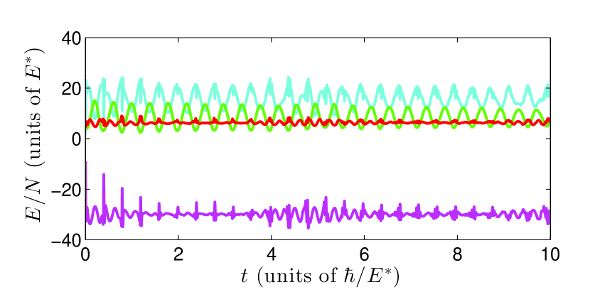
Figure 3: Time evolution of the various components of the energy per particle for $N=10$. The red, green, cyan, and magenta lines represent the interaction, trapping, kinetic, and ionic energy per particle, respectively.

The collapse and revival behavior can also be observed in the long time dynamics of the atomic density. Figure 4 shows the disappearance of the ionic oscillation during the time interval $[1.5,3.5]\hbar/E^{*}$ and its recurrence around $t\approx 4.0\,\hbar/E^{*}$. This effect seems to be directly connected to the loss and regain of spatial coherence between the inner and outer density fraction which can be observed in the snapshots of the one-particle density matrix at times $t=0.54\,\hbar/E^{*}$ (left panel), $t=2.20\,\hbar/E^{*}$ (middle panel), and $t=4.61\,\hbar/E^{*}$ (right panel) in Fig. 4. Below, we will understand the relation between the ionic oscillation and the spatial coherence in detail through the singlet-doublet analysis.

Figure 4: (Top panel) Time evolution of the one-particle density $\rho(z,t)$ for $N=10$. Snapshots of the one-particle reduced density matrix $\rho(z,z^{\prime},t)$ (lower panels) at times $t=0.54\,\hbar/E^{*}$ (left panel), $t=2.20\,\hbar/E^{*}$ (middle panel), and $t=4.61\,\hbar/E^{*}$ (right panel) which are indicated in the main top panel as white vertical lines ($\hbar/E^{*}=0.39\,\mathrm{m}\mathrm{s}$ for ${}^{87}\mathrm{Rb}$ atoms).

Let us now discuss the frequencies that are involved in the dynamics. To this aim, we investigate the fidelity defined by the overlap of the many-body wavefunction at time $t_{0}=0$ with the one at time $t$ Zanardi and Paunković (2006):

$$F(t)=|\langle\Psi(0)|\Psi(t)\rangle|^{2}.$$ (26)

Since this fidelity $F(t)$ can be understood as the expectation value of the time-evolution operator, thus an $N$-body operator, its Fourier transform contains information of all involved excited eigenstates of the interacting $N$ atom system. Due to the discrete nature of the spectrum and because in our numerical simulations the propagation time $T$ is finite, it turns out to be more efficient for the computation of the Fourier transform to use the compressed sensing (CS) method Donoho (2006); Candes and Tao (2006). With compressed sensing, one can indeed obtain a resolution in frequency space better than $\Delta\omega=\frac{2\pi}{T}$ Candes et al. (2006). To this end, we have used the matlab package “SPGL1” for compressed sensing from Ref. van den Berg and Friedlander (2007). The algorithms used in this package can be found in Refs. van den Berg and Friedlander (2008, 2011). In Fig. 5, we show the Fourier transform $F(\omega)$ of the fidelity (red continuous line). Several prominent resonances become apparent. We observe one dominant mode at a frequency $\omega\approx 34\,E^{*}/\hbar$. This corresponds to the ionic oscillation frequency. In contrast, the harmonic frequency can not directly be found in the spectrum. Furthermore, we see that modes with high frequency are excited and seem to have an equidistant spacing. In addition to this, there is a low energy mode around $\omega\approx 15\,E^{*}/\hbar$, whose origin we will explain in the subsequent sections.

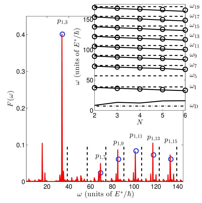
Figure 5: (Main panel) Excitation spectrum for $N=5$ and $g=2E^{*}R^{*}$. The red line represents the actual Fourier spectrum of the fidelity $F(t)$. The blue circles mark the single-particle energies (see text). We indicate the corresponding dominant singlet $p_{kq}$ at each peak by the label $p_{i,j}$ for the sake of better readability. The dashed vertical lines illustrate the non-interacting limit, thus correspond to $g=0$. Note that $p_{1,5}$ is hard to identify due to its small amplitude. (Inset) Prominent resonances of the spectrum $F(\omega)$ in dependence of $N$. The black solid lines are extracted from the Fourier transform of the fidelity $F(t)$. The circles indicate the resonance positions obtained from our singlet theory (see text). Further, the excitation energies for the non-interacting case (g=0) $\hbar\omega_{i}=\epsilon_{i}-\epsilon_{1}$ (dashed lines), $\hbar\omega_{\mathrm{I}}=\epsilon_{3}-\epsilon_{1}$ (lowest dashed line), and $\hbar\omega_{\mathrm{D}}=2(\epsilon_{2}-\epsilon_{1})$ (dashed dotted line) are shown.

III.2 Singlet Dynamics

Let us start the analysis of the many-body spectrum in terms of the singlets. Therefore, we choose from here on the non-interacting single-particle functions $\phi^{0}_{j}(x)$ as the basis $\phi_{j}(x)$ in which the clusters are expressed. In general, the identification of the modes corresponding to the observed resonances is a very complicated task. Nevertheless, we were able to identify the most important modes by linearizing the equation of motion for the singlets [see Eqs. (19) and (20), and App. B]. The obtained energies together with the “exact” spectrum belonging to the Fourier transform of the fidelity [see Eq. (26)] are shown in Fig. 5 (blue circles). One observes a very good agreement of the obtained peak positions with the Fourier spectrum of $F(t)$ (red continuous line). On the other hand, the relative heights of the peaks can be only obtained approximatively by our singlet theory (see App. B) showing qualitative agreement with the Fourier spectrum. Further, we can identify which singlet has the dominant contribution to a certain resonance (see App. B for details). This dominant singlet is indicated in Fig. 5 at the corresponding peak.

We find that the most dominant frequency corresponds to $p_{13}=\langle\hat{a}^{\dagger}_{1}\hat{a}^{{\color[rgb]{1,1,1}\dagger}}_{3}\rangle$ excitations. These are coherences between the number states $|N,0,0,...\rangle$ and $|N-1,0,1,0,...\rangle$ (in the basis of the non-interacting single-particle states $\phi^{0}_{j}(z)$) which oscillates with the frequency $\omega_{\mathrm{I}}=(\epsilon_{3}-\epsilon_{1})/\hbar=38.7\,E^{*}/\hbar$ for $g=0$. Thus, the ionic oscillation corresponds to an oscillation between a bound state and the first trap state (see also the oblique magenta arrows in Fig. 1). Hence, it connects the inner part of the atomic cloud with the outer fraction establishing spatial coherence between them as we have seen in Fig. 4. Moreover, this mode induces, as we will see in the following, population transfer between the inner and the outer atomic fraction. On the other hand, the harmonic oscillation can not be attributed to a single resonance, because no resonance shows up at its frequency. Nevertheless, we can understand its origin. We note that singlets $\langle\hat{a}^{\dagger}_{1}\hat{a}^{{\color[rgb]{1,1,1}\dagger}}_{i}\rangle$ with $i=5,7,9,...$ to very high $i$ are excited and therefore present in $F(\omega)$. They correspond to oscillations between the numberstate $|N,0,0,...\rangle$ and the states with $|N-1,0,...,0,1,0,...\rangle$, where a single particle is excited to the $i$th state and thus they oscillate, for $g=0$, with frequencies $\omega_{i}=(\epsilon_{i}-\epsilon_{1})/\hbar$ with $i=5,7,9,..$ (note that excitations into states with $i$ even are symmetry forbidden). These frequencies are shown in Figs. 5 as dashed lines. Since the difference between two neighboring resonances is approximatively constant $(\omega_{i+2}-\omega_{i})\approx 2\omega_{0}$ due to the equidistant spacing of the energy levels in the harmonic trap, all of these singlets are in phase again after a time $T\approx\pi/\omega_{0}\approx 0.4\hbar/E^{*}$. Although this approximation does not work perfectly at all times, because of the presence of the ionic potential, the harmonic oscillation is visible for the entire simulation time due to the contribution of high energy modes which are only slightly affected by the presence of the ion. Nevertheless, the damping of the harmonic oscillation, visible in the trap energy (see also Fig. 3, green line), can be attributed to the induced slight dephasing.

In the inset of Fig. 5, the resonance positions in dependence of the particle number $N$ are shown. We observe that the peaks which can be associated to a coherence $p_{1j}$ shift to smaller energies for growing $N$. Our singlet theory is perfectly able to capture this behavior. Therefore, the shift of resonances can be understood as a mean-field phenomenon which effectively renormalizes the singlet resonances. Importantly, we numerically find that the property of equidistant spacing between the single-particle modes seems to be nearly untouched by the interaction and, as a consequence, the harmonic oscillation is essentially unaffected.

The singlet theory explains most of the modes found in the Fourier spectrum $F(\omega)$. The low energy resonance at $\omega\approx 15.5\,E^{*}/\hbar$, however, does not appear in the singlet spectrum. Moreover, a closer inspection of the inset of Fig. 5 shows that this mode has the tendency of an increasing energy as the number of bosons increases, which is the opposite behavior of the other resonances. We show in the following that this resonance can be attributed to correlations which are dynamically build-up during the temporal evolution. To do so we have first to understand the coupling between the singlets and the doublets.

Towards that end, we proceed further with the analysis of the dynamical evolution of the singlets. In Fig. 6, the coherences $p_{13}$, $p_{1\mathrm{T}}=\sum_{k>3}p_{1k}$, and the occupations $f_{1}$, $f_{2}$, $f_{\mathrm{T}}=\sum_{k>3}f_{k}$ are shown. As stated beforehand, the coherence $p_{13}$ oscillates with the frequency of the ionic oscillation. From the time evolution of the ionic energy (see Fig. 3), one expects in addition the collapse and revival behavior. Here we see that for $N=2$ (lower left panel), the absolute value of $p_{13}$ is nearly constant, while collapse and revival become clearly visible for $N=10$ (lower right panel). The coherence between the first bound and the trap states, $p_{1\mathrm{T}}$, shows the aforementioned rephasing behavior in the distinct peaks with $T\approx\pi/\omega_{0}\approx 0.4\hbar/E^{*}$ periodicity. The damping is also visible here for $N=10$, but, importantly, the peaks are still very pronounced enabling the harmonic oscillation to be unaffected. Turning our attention to the dynamics of the occupations (Fig. 6, upper panels), we can identify that the population of the bound states, thus the ion population $f_{\mathrm{I}}=f_{1}+f_{2}$, is about $80-90\%$, and therefore only about $10\%-20\%$ of the particles are emitted into the trap by the “ionization process”. Furthermore, a population transfer between the two bound states occurs (upper left panel). For larger $N$ (upper right panel), also transfer to and from the trap population (green line) becomes visible with a rate equal to the frequency of the ionic oscillation.

An inspection of Eq. (20) reveals that the population transfer between the bound state $\phi^{0}_{1}$ and the trap states is mediated by coherences, primarily by $p_{13}$, because it has the highest contribution in the Fourier spectrum $F(\omega)$ (see also Fig. 5), explaining its oscillation with the frequency of the ionic oscillation. In contrast, the dynamical evolution of $f_{2}$ has to be induced by the correlations $\Gamma_{22}$, since all coherences in question vanish. Hence, the population transfer from the state $\phi^{0}_{1}$ to the state $\phi^{0}_{2}$ would not take place in a mean-field scenario, thus it is a clear signature of a genuine many-body effect. We also note that the frequency of this population transfer is $\omega\approx 8.2\,E^{*}/\hbar$ for $N=2$ which matches very well to the position of the additional low energy peak seen in the inset of Fig. 5. Further, the larger $N$ is, the faster the transfer process between the first bound and the trapped states happens which fits to the shift of the low energy resonance to larger energies visible in Fig. 5. We therefore show, in the next section, which doublets play an important role for this oscillation and to which process/mode it corresponds. Further, we will explain the origin of the collapse and revival of the ionic oscillation.

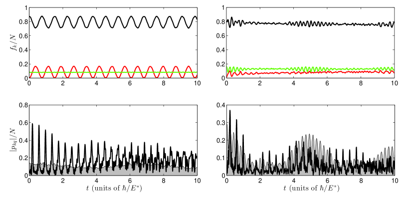
Figure 6: Time evolution of the singlets for $N=2$ (left panels) and $N=10$ (right panels). In the upper panels, the occupations $f_{k}$ are shown: $f_{1}$ (black line), $f_{2}$ (red line), and $f_{\mathrm{T}}$ (green line). Further, the absolute values of the most important coherences $p_{kq}$ are plotted in the lower panel: $p_{1\mathrm{T}}$ as a black line, and $p_{13}$ as a gray shaded area (for better visibility).

III.3 Doublet Dynamics

In order to understand the observed collapse and revival phenomena and the incoherent population transfer, we need to investigate the dynamical evolution of the doublets. For the sake of clarity, we classify the most important doublets (see definition in Sec. II.2.2) into incoherent doublets $g_{kkkk}$, $g_{kqkq}$, and coherent doublets $g_{kkqq}$, $g_{kqkk}$. This separation is justified by the fact that the incoherent doublets are always real-valued quantities, and therefore do not contribute to the dynamics of the singlet occupations [see Eq. (20)]. Moreover, the doublets have the properties $g_{kqk^{\prime}q^{\prime}}=g_{k^{\prime}q^{\prime}kq}^{*}$ and $g_{kqk^{\prime}q^{\prime}}=g_{kqq^{\prime}k^{\prime}}=g_{qkk^{\prime}q^{\prime}}=g_{qkq^{\prime}k^{\prime}}$. Therefore, we can identify, noting that only correlations involving states up to $k=3$ are contributing to the system dynamics, the most important classes of correlations: incoherent $\{g_{1111},g_{2222},g_{3333},g_{1212},g_{1313}\}$ and coherent $\{g_{1122},g_{1133},g_{2233},g_{1211},g_{2122},g_{1311},g_{3133},g_{2322},g_{3233}\}$. In Fig. 7, we show for $N=2$ (left panels) and $N=10$ (right panels) only those doublets of the incoherent (upper panels) and the coherent (lower panels) doublets which are considerably occupied. At first, we observe that, even though we start in an essentially uncorrelated state, very quickly a tremendous amount of correlations is created in the course of the temporal evolution. With the help of these correlations, we are now able to answer the remaining open questions concerning the dynamical evolution of the system.

In order to understand the population transfer between the states $\phi^{0}_{1}$ and $\phi^{0}_{2}$, we have to identify the correlations $g_{qkk^{\prime}q^{\prime}}$ contributing to $\Gamma_{11}$ and $\Gamma_{22}$. The coherent doublets $g_{1122}$ ($g_{2211}$) is the only correlation in question which can be understood by inspecting Eq. (22) and Fig. 7. Comparing Figs. 6 and 7 (left panels), we see that they are build up and decay with the frequency of the population transfer between the state $\phi^{0}_{1}$ to the state $\phi^{0}_{2}$. Since $g_{1122}$ and $g_{2211}$ which drive $\Gamma_{11}$ and $\Gamma_{22}$, respectively, are by $\pi$ out of phase ($g_{1122}=g_{2211}^{*}$), they induce the population transfer between those two bound states. Thus, we can understand these coherent doublets as mediators for the population transfer. Further, we can now identify the low energy mode in the spectrum of Fig. 5 as a coherent oscillation between the numberstates $|N,0,...\rangle$ and $|N-2,2,0,...\rangle$ which corresponds to a two-particle excitation. In the non-interacting case, this mode would therefore oscillate with a frequency $\omega_{\mathrm{D}}=2(\epsilon_{2}-\epsilon_{1})/\hbar\approx 7.4\,E^{*}/\hbar$ indicated by a dashed dotted line in the inset of Fig. 5. Here we can understand the following: First, this oscillation can not be seen in single-particle quantities like the one-body reduced density matrix. Second, this is also the reason why we could not explain the low energy peak by our singlet theory. Third, any mean-field approach would not be able to capture the associated dynamics. For example, in a GP theory the population transfer from $|N,0,...\rangle$ to $|N-2,2,0,...\rangle$ would be not possible, because in a general GP state $(\sum_{k}c_{k}\hat{a}^{\dagger}_{k})^{N}|\mathrm{vac}\rangle$ contributions from odd states are symmetry forbidden as long as only GP states with parity symmetry are considered.

Finally, we would like to discuss possible reasons for the collapse and revival behavior of the ionic oscillation occurring for larger $N$. The impact of the doublets onto the singlet $p_{13}$ is contained in $\Gamma_{13}$. Even if many doublets contribute to $\Gamma_{13}$, we can identify the responsible doublet by inspecting Fig. 7 (right panels). We observe that exactly at the times when the coherent doublets $g_{1133}$ are present, the ionic oscillation is strongly suppressed whereas when $g_{1133}$ nearly vanishes the ionic oscillation reappears (compare Figs. 3, 4, and 6). Therefore, the doublet $g_{1133}$ is the main source of loss of the coherence $p_{13}$. Consequently, this doublet is responsible for the loss of spatial coherence between the inner and the outer density fraction during the dynamics, as it can be seen in Fig. 4. Nevertheless, the build-up of $g_{1133}$ does not only act as a source of damping for the singlet coherences, since the coherences $p_{13}$ recur when the value of $g_{1133}$ is reduced again. Further, we note that $g_{1133}$ ($g_{3311}$) is also present in $\Gamma_{11}$ ($\Gamma_{33}$) such that also the collapse and revival in the population transfer can be attributed to this coherent doublet.

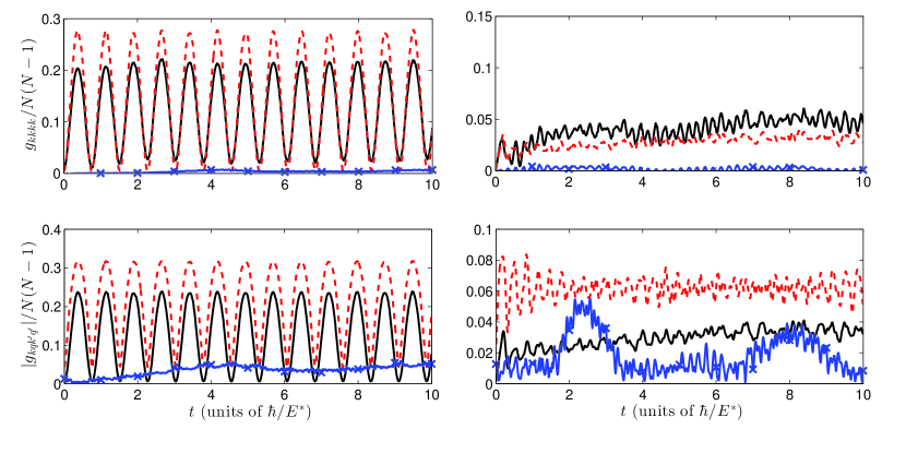
Figure 7: Time evolution of the most important doublets for $N=2$ (left panels) and $N=10$ (right panels). In the upper panels, the incoherent doublets $g_{1111}$ (black solid line), $g_{2222}$ (red dashed line), and $g_{3333}$ (blue line with crosses) are shown while the absolute values of coherent doublets $g_{1221}$ (black solid line), $g_{1122}$ (red dashed line), and $g_{1133}$ (blue line with crosses) are shown in the two lower panels.

IV Convergence Analysis

In the following, we briefly discuss the quality of our data and to which extend advanced tools as MCTDHB in the description of the dynamical behavior of such quantum systems are indeed necessary. To this aim, we inspect the natural populations [see Eq. (4)] which provide an assessment of the degree of fragmentation of the system Penrose and Onsager (1956). Further, one can use them to systematically judge the convergence of our result to the exact solution of the many-body quantum system Beck et al. (2000).

Figure 8: Natural populations $\lambda_{j}(t)$ exemplarily for $N=10$ particles on a logarithmic scale. Note that the $\lambda_{j}$ are by definition ordered such that $\lambda_{1}>\lambda_{2}>...>\lambda_{m}$ for all times.

In Fig. 8, the evolution of the natural populations exemplarily for $N=10$ particles is shown. We see that even if the initial state is nearly condensed, thus describable in the GP framework, depletion from the condensate state is created very quickly during the time evolution. Therefore, a GP description would be inaccurate and a multi-orbital description becomes unavoidable. Here we are using $m=6$ single-particle orbitals. The contribution of the lowest natural orbital (smallest natural population) stays below $1\%$ such that only natural orbitals with even smaller contribution are expected to be not taken into account by truncating the Hilbert space. One could further speculate that in such cases a multi-orbital mean-field description might be sufficient. However, this is not the case and we stress that the non-steady behavior of the natural populations implies the necessity to go beyond a mean-field description Krönke (2015). Therefore, the utilization of MCTDHB is essential to capture the full correlated quantum dynamics of the system.

V Conclusions and Outlook

We have investigated the dynamics of a trapped cloud of $N$ interacting bosons after the sudden creation of a static ion. Thereby, most of the atoms are quickly captured in the bound states of the atom-ion potential, while the remaining atomic fraction is emitted into the trap. We were able to understand the subsequent dynamics and the many-body spectrum in detail by means of an underlying singlet-doublet theory.

Our atom-ion hybrid system exhibits, apart from the harmonic oscillation, that is, a density oscillation within the external harmonic confinement, an additional density oscillation which we were able to attribute to a coherent oscillation between a bound state and a trap state. This coherent oscillation results in the spatial coherence between the inner and outer density fraction. It also allows for population transfer between bound and trap states such that the fraction of atoms in the bound states becomes time-dependent. In contrast to the harmonic oscillation, this ionic oscillation shows a particle number dependence. Furthermore, we showed that, even though the atoms are weakly interacting, strong correlations are build-up during the temporal evolution. These correlations lead to population transfer between the bound states and show up as a strong doublet resonance in the many-body spectrum. Besides this, the correlations induce a periodic suppression of coherence between the inner and the outer fraction which gives rise to collapse and revival of the ionic oscillation on longer time scales.

The impact of the ion onto the bosonic cloud dynamics can be summarized as follows: Apart from the accumulation of atoms on both sides of the ion while depleting the cloud at the ion position, the ion induces a coherent oscillation between the bound states and the trap states. The oscillation essentially arises because of the additional scales present in the system. Indeed, this can be easily seen in the non-interacting case ($g=0$) and taking the limit of small trapping frequency $\omega_{0}\rightarrow 0$. In this case, the frequency of the ionic oscillation converges to the non-interacting single-particle energy $\epsilon_{1}$ of the lower bound state (see Sec. II.1 for definition) which, thus, sets effectively a lower bound to the frequency of the ionic oscillation. Hence, although we have chosen a tight trap, which is numerically convenient to resolve the dynamics in a finite system, the ionic oscillation would be present with a frequency on the same order of magnitude for a weak confinement, too.

The present work can be viewed as a further step towards the simulation of the dynamics of the hybrid atom-ion system in the ultracold regime. The fact that quasi one-dimensional quantum Bose gases are routinely realized in several laboratories and given the recent advances in optical trapping of ions, puts the experimental realization of the hybrid system considered here within reach. Furthermore, since the multilayer extension of our method (ML-MCTDHB) is especially designed for the simulation of mixtures, we plan to investigate the impact of the ionic motion onto the ground state and the dynamical evolution of the bosonic ensemble in the nearer future. This will be done by treating the ion quantum mechanically as well. Due to the attractive inter-particle interaction, these future studies can reveal the dynamical formation of molecular ions as predicted in Ref. Côté et al. (2002). Furthermore, it would be of interest to study the energy transfer between ionic and atomic degrees of freedom in order to understand, for example, sympathetic cooling of the ion in the atomic cloud in more detail.

VI Acknowledgements

JS thanks Sven Krönke, Lushuai Cao, and Valentin Bolsinger for many discussions. This work has been financially supported by the excellence cluster ’The Hamburg Centre for Ultrafast Imaging - Structure, Dynamics and Control of Matter at the Atomic Scale’ of the Deutsche Forschungsgemeinschaft.

Appendix A Derivation of Clusters from Density Matrices

The $M$-particle clusters can be calculated via the $M$-particle reduced density matrices. Let us start with the time-dependent one-particle reduced density matrix which describes the spatial density and coherence of the system. We express it in terms of the natural orbitals $\Phi_{j}$ and the natural populations $\lambda_{j}$ as

$$\rho(x,x^{\prime},t)=\sum_{j}\lambda_{j}(t)\Phi_{j}^{*}(x,t)\Phi_{j}(x^{\prime},t).$$ (27)

If we now expand the natural orbitals in an arbitrary single-particle basis $\phi_{j}(x)$

$$\Phi_{j}(x,t)=\sum_{k}c_{jk}(t)\phi_{k}(x)$$ (28)

with

$$c_{jk}(t)=\int\phi^{*}_{k}(x)\Phi_{j}(x,t)\mathrm{d}{x}$$ (29)

and express also $\rho(x,x^{\prime},t)$ in this basis

$$\rho(x,x^{\prime},t)=\sum_{k,q}\phi_{k}^{*}(x)\phi_{q}(x^{\prime})\langle\hat{a}^{\dagger}_{k}\hat{a}^{{\color[rgb]{1,1,1}\dagger}}_{q}\rangle,$$ (30)

we can identify the single-particle cluster as

$$\langle\hat{a}^{\dagger}_{k}\hat{a}^{{\color[rgb]{1,1,1}\dagger}}_{q}\rangle=\sum_{j}c_{jk}^{*}(t)\lambda_{j}(t)c_{jq}(t).$$ (31)

Here $\hat{a}^{\dagger}_{k}$ and $\hat{a}^{{\color[rgb]{0.8,0.8,0.8}\dagger}}_{k}$ are the creation an annihilation operators of the single particle basis $\phi_{k}(x)$. In the same manner, we can proceed in order to derive the two-particle clusters. By defining the expansion coefficients as

$$d_{kq}^{j}(t)=\int\phi^{*}_{k}(x_{1})\phi^{*}_{q}(x_{2})\Phi_{j}(x_{1},x_{2},t)\mathrm{d}{x_{1}}\mathrm{d}{x_{2}},$$ (32)

where now $\Phi_{j}(x_{1},x_{2},t)$ are the geminals, that is, the eigenfunctions of the two-body density matrix, we obtain the following expression for the two-particle clusters

$$\langle\hat{a}^{\dagger}_{k}\hat{a}^{\dagger}_{q}\hat{a}^{{\color[rgb]{1,1,1}\dagger}}_{q^{\prime}}\hat{a}^{{\color[rgb]{1,1,1}\dagger}}_{k^{\prime}}\rangle=\sum_{j}d_{qk}^{j*}(t)\gamma_{j}(t)d_{k^{\prime}q^{\prime}}^{j}(t).$$ (33)

Appendix B Linearized Singlet Dynamics

In order to derive the energy spectrum of the singlets, we need to linearize the equations of motion (19) and (20). Even though such an approximation can not be able to describe the full dynamics, we should be able to predict the spectrum of the singlets rather accurately. To this end, we write the singlets as

$$\langle\hat{a}^{\dagger}_{i}\hat{a}^{{\color[rgb]{1,1,1}\dagger}}_{j}\rangle(t)=\langle\hat{a}^{\dagger}_{i}\hat{a}^{{\color[rgb]{1,1,1}\dagger}}_{j}\rangle_{0}+\delta\langle\hat{a}^{\dagger}_{i}\hat{a}^{{\color[rgb]{1,1,1}\dagger}}_{j}\rangle(t),$$ (34)

where $\langle\hat{a}^{\dagger}_{i}\hat{a}^{{\color[rgb]{1,1,1}\dagger}}_{j}\rangle_{0}$ is the time-independent mean value of $\langle\hat{a}^{\dagger}_{i}\hat{a}^{{\color[rgb]{1,1,1}\dagger}}_{j}\rangle(t)$ and $\delta\langle\hat{a}^{\dagger}_{i}\hat{a}^{{\color[rgb]{1,1,1}\dagger}}_{j}\rangle(t)$ is a small time-dependent fluctuation. By neglecting the terms quadratic in $\delta\langle\hat{a}^{\dagger}_{i}\hat{a}^{{\color[rgb]{1,1,1}\dagger}}_{j}\rangle$, we get a system of linear differential equations for $\delta\langle\hat{a}^{\dagger}_{i}\hat{a}^{{\color[rgb]{1,1,1}\dagger}}_{j}\rangle$. We obtain

$$i\hbar\frac{\mathrm{d}}{\mathrm{d}t}\delta\langle\hat{a}^{\dagger}_{i}\hat{a}^{{\color[rgb]{1,1,1}\dagger}}_{j}\rangle= \sum_{kq}\Big{[}\tilde{\epsilon}_{jq}^{0}\delta_{ki}-\tilde{\epsilon}_{ik}^{0*}\delta_{qj}$$

$$+2\sum_{k^{\prime}}V_{kjk^{\prime}q}\langle\hat{a}^{\dagger}_{i}\hat{a}^{{\color[rgb]{1,1,1}\dagger}}_{k^{\prime}}\rangle_{0}$$

$$-2\sum_{k^{\prime}}V_{qk^{\prime}ik}\langle\hat{a}^{\dagger}_{k^{\prime}}\hat{a}^{{\color[rgb]{1,1,1}\dagger}}_{j}\rangle_{0}$$

$$+(V_{kkki}+\sum_{q^{\prime}}V_{q^{\prime}kki}\langle\hat{a}^{\dagger}_{q^{\prime}}\hat{a}^{{\color[rgb]{1,1,1}\dagger}}_{k}\rangle_{0})\delta_{jq}$$

$$-(V_{jqqq}+\sum_{q^{\prime}}V_{jqqq^{\prime}}\langle\hat{a}^{\dagger}_{q}\hat{a}^{{\color[rgb]{1,1,1}\dagger}}_{q^{\prime}}\rangle_{0})\delta_{ik}$$

$$+V_{kqqi}\langle\hat{a}^{\dagger}_{q}\hat{a}^{{\color[rgb]{1,1,1}\dagger}}_{j}\rangle_{0}-V_{jkkq}\langle\hat{a}^{\dagger}_{i}\hat{a}^{{\color[rgb]{1,1,1}\dagger}}_{k}\rangle_{0}\Big{]}\delta\langle\hat{a}^{\dagger}_{k}\hat{a}^{{\color[rgb]{1,1,1}\dagger}}_{q}\rangle$$

$$+\tilde{\Gamma}_{ij}$$ (35)

where $\tilde{\epsilon}_{ij}^{0}=\epsilon_{i}\delta_{ij}+2\sum_{kq}V_{kijq}\langle\hat{a}^{\dagger}_{k}\hat{a}^{{\color[rgb]{1,1,1}\dagger}}_{q}\rangle_{0}$ and $\Gamma_{ij}^{\mathrm{B}0}$ coincides with the definitions of $\Gamma_{ij}^{\mathrm{B}}$, but with the mean values of the singlets inserted, whereas $\tilde{\Gamma}_{ij}$ is defined as

$$\tilde{\Gamma}_{ij}=\Gamma_{ij}+\Gamma_{ij}^{\mathrm{B}0}+\sum_{q}\left[\tilde{\epsilon}_{jq}^{0}\langle\hat{a}^{\dagger}_{i}\hat{a}^{{\color[rgb]{1,1,1}\dagger}}_{q}\rangle_{0}-\tilde{\epsilon}_{iq}^{0*}\langle\hat{a}^{\dagger}_{q}\hat{a}^{{\color[rgb]{1,1,1}\dagger}}_{j}\rangle_{0}\right].$$ (36)

Here we used Eq. (25) for the correlations $\Gamma_{ij}^{B}$. This is an important step because in case the doublets are negligible it decouples the singlets dynamics from any other time-dependent driving such that the many-body system can be described by singlets only. Finally, Eq. (35) can be rewritten in matrix form as

$$i\hbar\frac{\mathrm{d}}{\mathrm{d}t}{\mathbf{S}}(t)=M{\mathbf{S}}(t)+\tilde{{\mathbf{\Gamma}}}(t).$$ (37)

such that the homogeneous solution can be expanded in terms of the eigenvalues $\nu_{n}$ and the left(L) or right (R) eigenvectors ${\mathbf{S}}_{n}^{\mathrm{L,R}}$ of the matrix $M$

$$M{\mathbf{S}}^{\mathrm{R}}_{n}=\nu_{n}{\mathbf{S}}^{\mathrm{R}}_{n},$$ (38)

and the imhomogeneous part can be found by means of the variation of the constant method leading to the full solution

$${\mathbf{S}}(t)=\sum_{n}\left[c_{n}+\int_{0}^{t}\frac{1}{i\hbar}e^{i\nu_{n}t^{\prime}/\hbar}{\mathbf{S}}^{\mathrm{L}*}_{n}\tilde{{\mathbf{\Gamma}}}(t^{\prime})\mathrm{d}{t^{\prime}}\right]{\mathbf{S}}^{\mathrm{R}}_{n}e^{-i\nu_{n}t/\hbar}.$$ (39)

The coefficients $c_{n}$ determine how strong the mode ${\mathbf{S}}^{\mathrm{R}}_{n}$ is excited and can be obtained by projecting the above solution onto the eigenvector basis, resulting in

$$c_{n}=e^{i\nu_{n}t/\hbar}{\mathbf{S}}^{\mathrm{L}*}_{n}{\mathbf{S}}(t)-\int_{0}^{t}\frac{1}{i\hbar}e^{i\nu_{n}t^{\prime}/\hbar}{\mathbf{S}}^{\mathrm{L}*}_{n}\tilde{{\mathbf{\Gamma}}}(t^{\prime})\mathrm{d}{t^{\prime}}.$$ (40)

In summary, we see that the linearized singlet equations provide us with the singlet resonances $\nu_{n}$ and the singlet modes ${\mathbf{S}}_{n}^{\mathrm{R}}$. We can derive these from the MCTDHB solution in the following way: Via Eq. (31), we can extract the dynamics of the singlets which we can use to derive the matrix $M$, and therefore the solution ${\mathbf{S}}(t)$. By diagonalizing $M$, we obtain the singlet energies and the dominant singlet in the eigenmodes (largest entry in the vector) shown in Fig. 5. Further, we can extract the oscillator strength $|c_{n}|^{2}$ by Eq. (40) which we can use as a measure for the relative height of the peaks in the many-body Fourier spectrum of $F(t)$ just by scaling them to the global maximum of the spectrum. Note that, Eq. (40) should be evaluated at small $t$ in order to allow the linear approximation.

References

- Huang and Yang (1957) K. Huang and C. Yang, Phys. Rev. 105, 767 (1957).
- Gross (1963) E. P. Gross, J. Math. Phys. 4, 195 (1963).
- Pitaevskii (1961) L. P. Pitaevskii, J. Exp. Theor. Phys. 13, 451 (1961).
- Pitaevskii and Stringari (2003) L. P. Pitaevskii and S. Stringari, Bose-Einstein Condensation (Oxford University Press, 2003).
- Pethick and Smith (2008) C. Pethick and H. Smith, Bose-Einstein Condensation in Dilute Gases, 2nd ed. (Cambridge University Press, 2008).
- Schollwöck (2011) U. Schollwöck, Ann. Phys. (N. Y.) 326, 96 (2011).
- Alon et al. (2008) O. E. Alon, A. I. Streltsov, and L. S. Cederbaum, Phys. Rev. A 77, 033613 (2008).
- Cao et al. (2013) L. Cao, S. Krönke, O. Vendrell, and P. Schmelcher, J. Chem. Phys. 139, 134103 (2013).
- Krönke et al. (2013) S. Krönke, L. Cao, O. Vendrell, and P. Schmelcher, New J. Phys. 15, 063018 (2013).
- Büchler and Blatter (2003) H. Büchler and G. Blatter, Phys. Rev. Lett. 91, 130404 (2003).
- Büchler (2011) H. P. Büchler, New J. Phys. 13, 093040 (2011).
- Stuhler et al. (2005) J. Stuhler, A. Griesmaier, T. Koch, M. Fattori, T. Pfau, S. Giovanazzi, P. Pedri, and L. Santos, Phys. Rev. Lett. 95, 150406 (2005).
- Lahaye et al. (2009) T. Lahaye, C. Menotti, L. Santos, M. Lewenstein, and T. Pfau, Reports Prog. Phys. 72, 126401 (2009).
- Seaton and Steenman-Clark (1977) M. J. Seaton and L. Steenman-Clark, J. Phys. B At. Mol. Phys. 10, 2639 (1977).
- Smith et al. (2005) W. W. Smith, O. P. Makarov, and J. Lin, J. Mod. Opt. 52, 2253 (2005).
- Zipkes et al. (2010) C. Zipkes, S. Palzer, C. Sias, and M. Köhl, Nature 464, 388 (2010).
- Schmid et al. (2010) S. Schmid, A. Härter, and J. H. Denschlag, Phys. Rev. Lett. 105, 133202 (2010).
- Härter et al. (2012) A. Härter, A. Krükow, A. Brunner, W. Schnitzler, S. Schmid, and J. H. Denschlag, Phys. Rev. Lett. 109, 123201 (2012).
- Cetina et al. (2012) M. Cetina, A. T. Grier, and V. Vuletić, Phys. Rev. Lett. 109, 253201 (2012).
- Krych and Idziaszek (2015) M. Krych and Z. Idziaszek, Phys. Rev. A 91, 023430 (2015).
- Joger et al. (2014) J. Joger, A. Negretti, and R. Gerritsma, Phys. Rev. A 89, 063621 (2014).
- Tomza et al. (2015) M. Tomza, C. P. Koch, and R. Moszynski, Phys. Rev. A 91, 042706 (2015).
- Côté et al. (2002) R. Côté, V. Kharchenko, and M. D. Lukin, Phys. Rev. Lett. 89, 093001 (2002).
- Goold et al. (2010) J. Goold, H. Doerk, Z. Idziaszek, T. Calarco, and T. Busch, Phys. Rev. A 81, 041601 (2010).
- Gerritsma et al. (2012) R. Gerritsma, A. Negretti, H. Doerk, Z. Idziaszek, T. Calarco, and F. Schmidt-Kaler, Phys. Rev. Lett. 109, 080402 (2012).
- Doerk et al. (2010) H. Doerk, Z. Idziaszek, and T. Calarco, Phys. Rev. A 81, 012708 (2010).
- Bissbort et al. (2013) U. Bissbort, D. Cocks, A. Negretti, Z. Idziaszek, T. Calarco, F. Schmidt-Kaler, W. Hofstetter, and R. Gerritsma, Phys. Rev. Lett. 111, 080501 (2013).
- Schurer et al. (2014) J. M. Schurer, P. Schmelcher, and A. Negretti, Phys. Rev. A 90, 033601 (2014).
- Kosloff and Tal-Ezer (1986) R. Kosloff and H. Tal-Ezer, Chem. Phys. Lett. 127, 223 (1986).
- Chin et al. (2010) C. Chin, R. Grimm, P. Julienne, and E. Tiesinga, Rev. Mod. Phys. 82, 1225 (2010).
- Huber et al. (2014) T. Huber, A. Lambrecht, J. Schmidt, L. Karpa, and T. Schaetz, Nat. Commun. 5, 5587 (2014).
- Idziaszek et al. (2007) Z. Idziaszek, T. Calarco, and P. Zoller, Phys. Rev. A 76, 033409 (2007).
- Idziaszek et al. (2009) Z. Idziaszek, T. Calarco, P. S. Julienne, and A. Simoni, Phys. Rev. A 79, 010702 (2009).
- Dirac (1930) P. A. M. Dirac, Math. Proc. Cambridge Philos. Soc. 26, 376 (1930).
- Frenkel (1934) J. Frenkel, Wave Mechanics, 1st ed. (Clarendon Press, Oxford, 1934).
- Sakmann et al. (2008) K. Sakmann, A. Streltsov, O. Alon, and L. S. Cederbaum, Phys. Rev. A 78, 023615 (2008).
- Kira and Koch (2006) M. Kira and S. W. Koch, Prog. Quantum Electron. 30, 155 (2006).
- Penrose and Onsager (1956) O. Penrose and L. Onsager, Phys. Rev. 104, 576 (1956).
- Beck et al. (2000) M. H. Beck, A. Jäckle, G. A. Worth, and H.-D. Meyer, Phys. Rep. 324, 1 (2000).
- Wyld and Fried (1963) H. Wyld and B. D. Fried, Ann. Phys. (N. Y.) 23, 374 (1963).
- Purvis and Bartlett (1982) G. D. Purvis and R. J. Bartlett, J. Chem. Phys. 76, 1910 (1982).
- Kira and Koch (2012) M. Kira and S. Koch, Semiconductor Quantum Optics (Cambridge University Press, 2012).
- Note (1) We note that this does not imply that the individual terms of the sum vanish.
- Note (2) The appearance of is due to the bosonic symmetry and the possibility for bosons to have an occupancy .
- Cederbaum and Streltsov (2003) L. S. Cederbaum and A. Streltsov, Phys. Lett. A 318, 564 (2003).
- Zanardi and Paunković (2006) P. Zanardi and N. Paunković, Phys. Rev. E 74, 031123 (2006).
- Donoho (2006) D. Donoho, IEEE Trans. Inf. Theory 52, 1289 (2006).
- Candes and Tao (2006) E. J. Candes and T. Tao, IEEE Trans. Inf. Theory 52, 5406 (2006).
- Candes et al. (2006) E. Candes, J. Romberg, and T. Tao, IEEE Trans. Inf. Theory 52, 489 (2006).
- van den Berg and Friedlander (2007) E. van den Berg and M. P. Friedlander, “{SPGL1}: A solver for large-scale sparse reconstruction,” (2007).
- van den Berg and Friedlander (2008) E. van den Berg and M. P. Friedlander, SIAM J. Sci. Comput. 31, 890 (2008).
- van den Berg and Friedlander (2011) E. van den Berg and M. P. Friedlander, SIAM J. Optim. 21, 1201 (2011).
- Krönke (2015) S. Krönke, Correlated Quantum Dynamics of Ultracold Bosons and Bosonic Mixtures: the Multi-Layer Multi-Configuration Time-Dependent Hartree Method for Bosons, Ph.D. thesis, Universität Hamburg (2015).