Numerical Study on In-Situ Prominence Formation by Radiative Condensation in the Solar Corona

Abstract

We propose an in-situ formation model for inverse-polarity solar prominences and demonstrate it using self-consistent 2.5-dimensional magnetohydrodynamics simulations, including thermal conduction along magnetic fields and optically thin radiative cooling. The model enables us to form cool dense plasma clouds inside a flux rope by radiative condensation, which is regarded as an inverse-polarity prominence. Radiative condensation is triggered by changes in the magnetic topology, i.e., formation of the flux rope from the sheared arcade field, and by thermal imbalance due to the dense plasma trapped inside the flux rope. The flux rope is created by imposing converging and shearing motion on the arcade field. Either when the footpoint motion is in the anti-shearing direction or when heating is proportional to local density, the thermal state inside the flux rope becomes cooling-dominant, leading to radiative condensation. By controlling the temperature of condensation, we investigate the relationship between the temperature and density of prominences and derive a scaling formula for this relationship. This formula suggests that the proposed model reproduces the observed density of prominences, which is 10–100 times larger than the coronal density. Moreover, the time evolution of the extreme ultraviolet emission synthesized by combining our simulation results with the response function of the Solar Dynamics Observatory Atmospheric Imaging Assembly filters agrees with the observed temporal and spatial intensity shift among multi-wavelength during in-situ condensation.

1 Introduction

Solar prominences are cool dense plasma clouds that form in the hot tenuous corona. Dense plasmas are sustained at the dipped (concave-up) structures of coronal arcade fields (Kippenhahn & Schlüter, 1957; Kuperus & Raadu, 1974). Prominences can be classified into two groups — normal- and inverse-polarity prominences — depending on their interior magnetic polarity with respect to the overlying arcade field. In normal-polarity prominences, the magnetic polarity matches that of the overlying arcade field. Normal-polarity prominences are typically modeled by the Kippenhahn–Schlüter (KS) model. In inverse-polarity prominences, the interior magnetic polarity opposes that of the overlying arcade field. This prominence group is described by the Kuperus–Raadu (KR) model, in which the lower half of the flux rope indicates the inverse-polarity. Both normal- and inverse-polarity prominences are observed in the solar atmosphere (Leroy et al., 1984).

An unsolved problem regarding prominences is the origin of their cool dense plasmas. Though several models have been proposed, the actual mechanism by which prominences form remains debatable (Mackay et al., 2010). One candidate mechanism for prominence formation is radiative condensation (Antiochos et al., 1999). Several models for triggering radiative condensation have been proposed and demonstrated by numerical simulations. One is the evaporation–condensation process (Mackay et al., 2010), in which evaporated flows from the chromosphere lead to radiative condensation in the coronal loops. The mechanism and constraints of this model have been investigated using one-dimensional hydrodynamics simulations (Karpen et al., 2006; Luna et al., 2012) and two-dimensional self-consistent magnetohydrodynamics (MHD) simulations (Xia et al., 2012). These studies have shown the formation of normal-polarity prominences categorized by the KS model, whereas Keppens & Xia (2014) showed that the evaporation–condensation model eventually evolved into the funnel prominence in which the flux rope structure is embedded.

Choe & Lee (1992) demonstrated the formation of a normal-polarity prominence by a different process. In their two-dimensional MHD simulations, the shearing motion at the footpoints of the potential arcade fields leads to radiative condensation due to the expansion of the arcade fields. Linker et al. (2001) demonstrated the formation of inverse-polarity prominences. In their simulations, the chromospheric plasmas are levitated as a result of flux rope formation by the magnetic cancellation and condensation occurs.

Condensation models triggered by evaporation or levitation rely on the injection of chromospheric plasmas. On the other hand, a recent observation of a prominence formation event showed no clear evidence of chromospheric plasma injection, and claimed the presence of in-situ condensation (Berger et al., 2012). Xia et al. (2014a) modeled in-situ condensation inside a flux rope by three-dimensional simulation, and showed that the features of prominences are well reproduced. Because they used the mechanically stable flux rope model obtained from the isothermal simulation (Xia et al., 2014b) and started their simulation with an ad hoc thermal imbalance, the process required to trigger the radiative condensation is still unclear.

In this study, we model the process from flux rope formation to radiative condensation using self-consistent 2.5-dimensional MHD simulations, including thermal conduction and radiative cooling. By comparing the results of multiple simulations with different settings regarding the formation model of flux rope and the coronal heating model, we discuss the condition for triggering radiative condensation and the possible relationship between the temperature and density of the prominence condensations.

Section 2 introduces our prominence formation model, and Section 3 describes the numerical simulation setup. The simulation results are presented in Section 4. The condition for triggering radiative condensation and a scaling formula from the possible temperature–density relationships are discussed in Section 5.

2 Possible processes for triggering in-situ condensation

The schematic picture of our model for triggering in-situ radiative condensation is presented as follows. Initially, the coronal arcade exists in thermal equilibrium (Fig. 1 (a)). The arcade field is transformed into a flux rope structure by converging and shearing motion (van Ballegooijen & Martens, 1989; Martens & Zwaan, 2001). The relatively dense plasmas in the lower corona due to stratification are trapped inside closed loops of the flux rope, where they are elevated into the upper corona (Fig. 1 (b)). The dense plasmas increase the radiative cooling in the flux rope, leading to thermal imbalance. Because the closed field lines are disconnected from the exterior region, the heat loss by radiative cooling inside the flux rope is not conducted outward, and radiative condensation can be triggered. (Fig. 1 (c)).

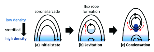
Figure 1: Schematic of a possible process of in-situ radiative condensation

3 Numerical Settings

To demonstrate the proposed model, we perform 2.5-dimensional MHD simulations, including thermal conduction along the magnetic field lines, radiative cooling, and gravity in a Cartesian ($x$,$y$) domain. To investigate the necessary condition for triggering radiative condensation, we test different direction of the converging and shearing motion for the formation of a flux rope and different coronal heating models.

3.1 Initial and boundary conditions

The corona model is set up in a rectangular box, in which the $x$- and $y$-axes are horizontal and vertical, respectively, and the $z$-axis is orthogonal to the $x$–$y$ plane. The corona is stratified under uniform temperature ($T_{\mathrm{cor}}=\mathrm{1MK}$) and gravity ($g_{\mathrm{cor}}=\mathrm{2.7\times 10^{4}~{}cm~{}s^{-2}}$) conditions,

$$\rho(y) = \rho_{\mathrm{cor}}\exp\left[-\frac{mg_{\mathrm{cor}}}{k_{B}T_{\mathrm{cor}}}y\right],$$ (1)

$$p(y) = \frac{k_{B}}{m}\rho(y)T_{\mathrm{cor}},$$ (2)

where $\rho_{\mathrm{cor}}=\mathrm{3.2\times 10^{-15}~{}g~{}cm^{-3}}$, $k_{B}$ is Boltzmann’s constant, and $m$ is the mean molecular mass. We set $m=m_{p}$ with $m_{p}$ being the proton mass. The force-free arcade field iss described as

$$B_{x} = -\left(\frac{2L_{a}}{\pi a}\right)B_{a}\cos\left(\frac{\pi}{2L_{a}}x\right)\exp\left[-\frac{y}{a}\right],$$ (3)

$$B_{y} = B_{a}\sin\left(\frac{\pi}{2L_{a}}x\right)\exp\left[-\frac{y}{a}\right],$$ (4)

$$B_{z} = -\sqrt{1-\left(\frac{2L_{a}}{\pi a}\right)^{2}}B_{a}\cos\left(\frac{\pi}{2L_{a}}x\right)\exp\left[-\frac{y}{a}\right],$$ (5)

where $B_{a}=3~{}\mathrm{G}$ is the field strength at the footpoint, $L_{a}=12~{}\mathrm{Mm}$ is the width, and $a=31~{}\mathrm{Mm}$ is the magnetic scale height of the arcade field. Initially, the system exists in mechanical equilibrium.

The left and right boundaries are subjected to symmetric (for $\rho,p,v_{y},B_{y}$) or anti-symmetric (for $v_{x},v_{z},B_{x},B_{z}$) boundary conditions. A free boundary condition is applied to the top. In the region below $y=0$, the converging and shearing motions are introduced. We test three types of the footpoint motions. One is the converging motion without shearing; the others are converging motion with shearing that increases the magnetic shear of the arcade field or with anti-shearing that decreases the shear of the arcade field. In all the cases, the velocity components $v_{x}$ and $v_{y}$ within this region are set as follows,

$$v_{x} = -v_{0}(t)\frac{x}{L_{a}/4},~{}v_{y}=0,~{}~{}(0\leq x<L_{a}/4,~{}y<0)$$ (6)

$$v_{x} = -v_{0}(t)\frac{(L_{a}-x)}{3L_{a}/4},~{}v_{y}=0,~{}~{}(L_{a}/4\leq x\leq L_{a},~{}y<0),$$ (7)

$$v_{0}(t)= v_{00},~{}~{}(0<t<t_{1})$$ (8)

$$v_{0}(t)= v_{00}(t_{2}-t)/(t_{2}-t_{1}),~{}~{}(t_{1}\leq t<t_{2})$$ (9)

$$v_{0}(t)= 0,~{}~{}(t\geq t_{2})$$ (10)

where $v_{00}=12~{}\mathrm{km/s}$, $t_{1}=1000~{}\mathrm{s}$, and $t_{2}=1500~{}\mathrm{s}$. In the case of no shearing motion, $v_{z}=0$. The shearing and the anti-shearing motions are set as follows,

$$v_{z} = \pm v_{0}(t)\frac{x}{L_{a}/4},~{}~{}(0\leq x<L_{a}/4,~{}y<0)$$ (11)

$$v_{z} = \pm v_{0}(t)\frac{(L_{a}-x)}{3L_{a}/4},~{}~{}(L_{a}/4\leq x\leq L_{a},~{}y<0)$$ (12)

where the plus and minus signs represent the shearing and anti-shearing motions, respectively. The magnetic fields are computed with the induction equation by coupling with the given converging and shearing motions. The magnetic fields at the bottom boundary are fixed to the initial state. The gas pressure and density are fixed by assuming hydrostatic equilibrium at a constant temperature of $T_{\mathrm{cor}}=10^{6}~{}\mathrm{K}$.

3.2 Basic equations

The basic equations are

$$\frac{\partial\rho}{\partial t}+\mbox{\boldmath$v$}\cdot\mbox{\boldmath$\nabla$}\rho=-\rho\mbox{\boldmath$\nabla$}\cdot\mbox{\boldmath$v$},$$ (13)

$$\frac{\partial e_{\mathrm{th}}}{\partial t}+\mbox{\boldmath$v$}\cdot\mbox{\boldmath$\nabla$}e_{\mathrm{th}}=-(e_{\mathrm{th}}+p)\mbox{\boldmath$\nabla$}\cdot\mbox{\boldmath$v$}+\mbox{\boldmath$\nabla$}\cdot\left(\kappa T^{5/2}\mbox{\boldmath$bb$}\cdot\mbox{\boldmath$\nabla$}T\right)-L,$$ (14)

$$e_{\mathrm{th}}=\frac{p}{\gamma-1},$$ (15)

$$\frac{\partial\mbox{\boldmath$v$}}{\partial t}+\mbox{\boldmath$v$}\cdot\mbox{\boldmath$\nabla v$}=-\frac{1}{\rho}\mbox{\boldmath$\nabla$}p+\frac{1}{4\pi\rho}\left(\mbox{\boldmath$\nabla$}\times\mbox{\boldmath$B$}\right)\times\mbox{\boldmath$B$}+\mbox{\boldmath$g$},$$ (16)

$$\frac{\partial\mbox{\boldmath$B$}}{\partial t}=-c\mbox{\boldmath$\nabla$}\times\mbox{\boldmath$E$},$$ (17)

$$\mbox{\boldmath$E$}=-\frac{1}{c}\mbox{\boldmath$v$}\times\mbox{\boldmath$B$}+\frac{4\pi\eta}{c^{2}}\mbox{\boldmath$J$},$$ (18)

$$\mbox{\boldmath$J$}=\frac{c}{4\pi}\mbox{\boldmath$\nabla$}\times\mbox{\boldmath$B$},$$ (19)

where $\mathrm{\kappa=2\times 10^{-6}~{}erg~{}cm^{-1}~{}s^{-1}~{}K^{-7/2}}$ is the coefficient of thermal conduction, $b$ is a unit vector along the magnetic field, and $\mbox{\boldmath$g$}=(0,-g_{\mathrm{cor}},0)$ is the gravitational acceleration and $\eta$ is the magnetic diffusion rate. The temperature is computed by the following equation of state,

$$T=\frac{m}{k_{B}}\frac{p}{\rho}.$$ (20)

For fast reconnection, we adopt the following form of the anomalous resistivity (e.g. Yokoyama & Shibata, 1994),

$$\eta= 0,~{}~{}~{}~{}~{}~{}~{}~{}~{}~{}~{}~{}~{}~{}~{}~{}~{}~{}~{}\left(J<J_{c}\right)$$ (21)

$$\eta= \eta_{0}\left(J/J_{c}-1\right)^{2},~{}~{}\left(J\geq J_{c}\right)$$ (22)

where $\eta_{0}=\mathrm{3.6\times 10^{13}~{}cm^{2}~{}s^{-1}}$ and $J_{c}=\mathrm{25~{}dyn^{1/2}~{}cm~{}s^{-1}}$. We restrict $\eta$ to $\eta_{\mathrm{max}}=\mathrm{18.0\times 10^{13}~{}cm^{2}~{}s^{-1}}$. $L$ in Eq. (14) represents the net cooling term, which is expressed as

$$L=n^{2}\Lambda(T)-H-\eta J^{2},$$ (23)

where $n=\rho/m$ is the number density, $\Lambda(T)$ is the radiative loss function of optically thin plasma, $H$ is the background heating rate, and $\eta J^{2}$ represents ohmic heating. We adopt a simplified radiative loss function in Fig. 2 (a) (Hildner, 1974) and simulate two different coronal heating models. In one model, the heating rate $H$ depends on the local magnetic energy density (magnetic pressure) at temperatures above the cutoff temperature $T_{\mathrm{c}}$ and is balanced out by the cooling rate when it falls below $T_{\mathrm{c}}$,

$$H= \alpha_{m}P_{m},~{}~{}\left(T\geq T_{\mathrm{c}}\right)$$ (24)

$$H= n^{2}\Lambda(T),~{}~{}\left(T<T_{\mathrm{c}}\right)$$ (25)

Initial thermal equilibrium required that

$$\alpha_{m}=\frac{n_{\mathrm{cor}}^{2}\Lambda(T_{\mathrm{cor}})}{B_{a}^{2}/8\pi}\exp\left[-2\left(\frac{mg_{\mathrm{cor}}}{k_{B}T_{\mathrm{cor}}}-\frac{1}{a}\right)y\right],$$ (26)

where $n_{\mathrm{cor}}=\rho_{\mathrm{cor}}/m=2.0\times 10^{9}~{}\mathrm{cm^{-3}}$. Selecting $a=k_{B}T_{\mathrm{cor}}/(mg_{\mathrm{cor}})$, we obtain $\alpha_{m}=6.2\times 10^{-4}~{}\mathrm{cm^{3}~{}s^{-1}}$ (i.e., a constant). Equation (25) prevents the temperature from decreasing below $T_{\mathrm{c}}$. In the other model, the heating rate $H$ depends on the local density and height at temperatures above $T_{\mathrm{c}}$ and balances with the cooling rate below the cutoff temperature $T_{\mathrm{c}}$.

$$H= \alpha_{d}(y)n,~{}~{}\left(T\geq T_{\mathrm{c}}\right)$$ (27)

$$H= n^{2}\Lambda(T).~{}~{}\left(T<T_{\mathrm{c}}\right)$$ (28)

For the initial thermal equilibrium, we have $\alpha_{d}(y)=n_{\mathrm{cor}}\Lambda(T_{\mathrm{cor}})\exp[-mg_{\mathrm{cor}}y/(k_{B}T_{\mathrm{cor}})]$ where $n_{\mathrm{cor}}\Lambda(T_{\mathrm{cor}})=1.1\times 10^{-13}~{}\mathrm{erg~{}s^{-1}}$. Note that ohmic heating is always much smaller than background heating in these settings. $T_{\mathrm{c}}$ is one of the model parameters. For each heating and shearing model, we vary $T_{\mathrm{c}}$ as $0.3$ MK, $0.4$ MK, and $0.5$ MK. The investigated cases are summarized in Table 1.

3.3 Numerical scheme and grid size

The numerical scheme is based on the CIP-MOCCT method (Kudoh et al., 1999). To prevent numerical oscillations in the advection term (left-hand side of Eqs. (13)–(16)), we apply the rational CIP scheme (Xiao et al., 1996), in which the rational function replaces the cubic function as an interpolation function of CIP. The thermal conduction, radiative cooling, and heating terms are included as source terms in non-advection phases of CIP method. Thermal conduction is explicitly solved by a second-order accurate slope-limiting method (Sharma & Hammett, 2007).

The required grid size for preventing numerical thermal instability can be estimated by the formula presented in Koyama & Inutsuka (2004). When applying this formula to our simulation, we assume that the density of the condensations is 10 times the coronal density,

$$\Delta<\frac{\lambda_{F}}{3}=\frac{1}{3}\sqrt{\frac{\kappa T_{\mathrm{c}}^{7/2}}{n_{\mathrm{c}}^{2}\Lambda(T_{\mathrm{c}})}},$$ (29)

where $\Delta$ is the grid size, $\lambda_{F}$ is the Field length, $T_{\mathrm{c}}$ is the cutoff temperature (also assume to be the temperature of condensations), and $n_{\mathrm{c}}=10n_{\mathrm{cor}}$ is the assumed density of condensations. Figure 2 (b) shows the required grid size against temperature. Under the constraint of Eq. (29), the grid size is determined to be $\Delta=$ 120 km, 60 km, and 30 km in the cases of $T_{\mathrm{c}}=$0.5 MK, 0.4 MK, and 0.3 MK, respectively. The horizontal grid size $\Delta x$ is uniform. The vertical grid size $\Delta y$ is uniform up to $y<24~{}\mathrm{Mm}$ and increases to $\Delta y=\mathrm{1.8\times 10^{3}~{}km}$ at $y>24~{}\mathrm{Mm}$ to ensure a sufficiently distant upper boundary.

Figure 2: Simplified radiative cooling functions and required grid sizes

4 Results

The right-most column of Table 1 shows our results in the presence of the radiative condensation. We find that the necessary condition for the radiative condensation is either anti-shearing motion or the heating proportional to the local density. Panels (a)–(d) of Fig. 3 are snapshots of the time evolution and Fig. 4 is the final state in case M1, which is a the typical case for the radiative condensation. The initial state exists in mechanical and thermal equilibrium (Fig. 3 (a)). Converging motion triggers reconnection above the PIL at $x=0$, and a flux rope is formed (Fig. 3 (b)). As the reconnection proceeds, the relatively dense plasmas in the lower corona are trapped inside the flux rope and lifted to the upper corona. The dense plasmas enhances radiative cooling in the flux rope, which overwhelms the background heating and leads to thermal imbalance (Fig. 3 (c)). Because thermal conduction works only along closed magnetic field lines of the flux rope, it can not compensate for the thermal imbalance. Consequently, radiative condensation is triggered, and the cool dense plasmas accumulates in the lower part of the flux rope (Fig. 3 (d)). Figure 4 (b) shows profiles of temperature, number density, and horizontal component of the magnetic field along the $y$-axis in the quasi–static state (Fig. 4 (a)). The temperature of the prominence corresponding to $T_{\mathrm{c}}$ is approximately $0.3~{}\mathrm{MK}$ in this case. The heating settings (Eqs. (25) and (28)) maintains the temperature of the cool dense plasmas at around $T_{\mathrm{c}}$. According to Fig. 4 (b), the magnetic polarity of the cool dense region opposes that of the initial arcade field. Figures 4 (a) and (b) clearly show that radiative condensation eventually establishes inverse-polarity prominence in the flux rope. Also, the high-density region (warm color region in the density plot of Fig. 4 (a)) resembles the tower prominence (Berger et al., 2012), and the low-density region surrounding the prominence (dark region in the same plot) can be regarded as the coronal cavity. Figure 5 shows each force at a time of $=$4250s. The mechanical quasi-static state is realized in the vertical direction. The upward magnetic tension force is balanced with the downward pressure gradient force and gravity, i.e., the prominence mass is supported mainly by the magnetic tension. This force balance system is also found in the parametric study by adiabatic MHD simulations of Hillier & van Ballegooijen (2013). Our result mostly corresponds to their case (e) of model 1 regarding the force balance, whereas the prominence density and plasma $\beta$ in our simulation are lower and higher than those in Hillier & van Ballegooijen (2013), respectively. They revealed that the magnetic tension force is given by the vertical stretching of the flux rope, and the curvature of the field lines inside the prominence can be smaller because the sufficiently large magnetic tension comes from the larger field strength by compression of the prominence mass. Our simulation realizes these features of prominence support as shown in Fig. 4 (a). Figures 6 shows the time evolution of case M5, which is a typical case with no radiative condensation. The flux rope is heated-up rather than cooled-down in this case.

case	Heating	Shearing	$T_{c}$ (MK)	Condensation
M1		$-$	0.3	Yes
M2		$-$	0.4	Yes
M3	$H=\alpha_{m}P_{m}$	$-$	0.5	Yes
M4		0	0.5	No
M5		$+$	0.5	No
D1		$-$	0.3	Yes
D2		$-$	0.4	Yes
D3	$H=\alpha_{d}\rho$	$-$	0.5	Yes
D4		0	0.5	Yes
D5		$+$	0.5	Yes

Table 1: The presence of radiative condensation in each case. The second column shows the heating model. The third column shows the shearing model: plus sign ($+$), minus sign ($-$), and 0 represent the shearing, anti-shearing, and no shearing cases, respectively. The fourth column shows the cutoff temperature. The fifth column shows the presence of condensation.

Figure 3: Panels (a)–(d) are snapshots of the time evolution in case M1. Colors represent temperature and density, white lines represent magnetic field lines, and arrows represent the velocity fields.

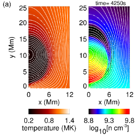
Figure 4: Panel (a) is the final state in case M1. Colors, white lines and arrows represent the same quantities as in Fig.3. Panel (b) shows the profiles of temperature, number density, and $B_{x}$ along the $y$-axis. The solid and dashed lines are the profiles in the final and initial states, respectively.

Figure 5: The vertical components of the forces along the $y$-axis. The dotted line, dashed line, and dot-dashed line represent the pressure gradient (the sum of the gas and magnetic pressure gradients), magnetic tension force, and gravity, respectively. The solid line represents sum of all the forces.

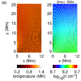
Figure 6: Panels (a)–(b) are snapshots of the time evolution in case M5. Colors and arrows denote the same quantities as those in Fig.3. Black lines represent magnetic field lines.

5 Discussion

As shown in Table 1, the radiative condensation occurs either when the anti-shearing motion is imposed or when the heating model is proportional to the density, i.e., $H=\alpha_{d}\rho$. The radiative condensation is triggered by the cooling-dominant thermal imbalance in the flux rope composed of the thermally isolated closed loops. The interior of the flux rope is relatively dense because of the converging motion as well as the initial stratification. Because the radiative cooling inside the flux rope is enhanced by the dense plasma, the cooling-dominant thermal imbalance is reasonable if the heating changes only slightly. Because we set the heating depending on the magnetic pressure (cases M1–M5, hereafter called M-cases) and local density (cases D1–D5, hereafter called D-cases), the change in heating rate is not negligible. In some cases (M5 and M6), a heating-dominant thermal imbalance is created and no condensations occur. In the following subsections, we discuss the mechanism for creating the cooling/heating-dominant thermal imbalance in the M- and D-cases. Then, our model is compared with previous theoretical studies and observations.

5.1 Thermal imbalance in M-cases

In M-cases where the heating rate is proportional to the magnetic pressure, the anti-shearing and shearing motion causes a larger discrepancy between the cooling and heating rates, establishing the cooling- and heating-dominant thermal imbalances, respectively. Figure 7 shows the cooling and heating rates along the $y$-axis at time=$500\mathrm{s}$ in case M3–M5. In case M3 (anti-shearing case), the cooling rate is the highest of the three cases, whereas the heating rate is the lowest. Case M5 (shearing case) has the opposite tendency, where the cooling rate is the lowest and the heating rate is the highest. We discuss how these tendencies are established from a perspective of the evolution of the magnetic field and its influence on the cooling and heating rates.

In the anti-shearing case, the flux rope is pushed upward by the reconnection and confined by the downward magnetic tension of the overlying arcade field. Figure 8 shows the vertical tension force along the $y$-axis at time=$500~{}\mathrm{s}$ in case M3 (anti-shearing), M4 (no shearing), and M5 (shearing). The downward magnetic tension force in the anti-shearing case is larger than those in the shearing and no shearing cases. The reason the anti-shearing case has the larger downward tension force is as follows: the shear angle is related to the height of the arcade field as

$$a=\frac{L_{a}}{\pi\cos\theta},$$ (30)

where $a$ is the arcade height, $\theta=\arctan(B_{z}/B_{x})$ is the shear angle against the positive $x$-axis in the $x$$z$-plane, $L_{a}$ is the arcade width, and we assume a linear force-free arcade field for simplicity. Equation (30) indicates that the reduction of magnetic shear by the anti-shearing motion makes the arcade field shorter. Due to the shrink of the arcade field, the flux rope in the anti-shearing case experiences a larger downward magnetic tension force.

The flux rope in the anti-shearing case is pinched by the overlying arcade field and pushed by the upward magnetic tension of the reconnected loops, leading to a density enhancement by compression. Figure 9 shows the time evolution of area and average density inside the dash-dotted line in Fig. 6. The average density is computed by dividing the total mass inside the dash-dotted line by the corresponding area. The total mass is almost the same between these three cases and is conserved after the flux rope is detached from the bottom boundary. In Fig. 9 (b), the anti-shearing case shows the enhancement of the average density. This result indicates that the density enhancement inside the flux rope in the anti-shearing case is due to the compression by the magnetic tension as well as the converging motion.

The anti-shearing motion lead to the higher cooling rate as well as the lower heating rate. The anti-shearing motion reduces the magnetic component parallel to the PIL, corresponding to $B_{z}$ in our simulations, and decreases the magnetic pressure, leading to the lowest heating rate. Thus, the interior of the flux rope in case M3 suffers from unstoppable cooling most efficiently. In case M5 (shearing case), on the other hand, the heating rate increases as the magnetic pressure increases, and the enhancement of the cooling rate is too small to overwhelm the heating rate. Eventually, the shearing motion is likely to establish the heating-dominant thermal imbalance, resulting only in the formation of hot flux rope. These results suggest that when the coronal heating depends on the magnetic energy density, the continuous shearing motion can not trigger the radiative condensation, whereas the temporary anti-shearing motion can indeed trigger it, leading to the prominence formation.

5.2 Thermal imbalance in D-cases

From the results of the D-cases in which the heating is proportional to the density, it is found that the cooling-dominant thermal imbalance can be achieved only by the difference between the heating and cooling rates in the dependence on the density. Figure 10 shows the cooling and the heating rates in the cases D3–D5. The cooling rate in case D3 (anti-shearing case) is highest because the density enhancement is largest in the anti-shearing case, as discussed in the previous subsection. Unlike case M3, however, the heating rate in case D3 is also highest. The combination of the higher cooling rate and the higher heating rate can be a disadvantage to enhancing the thermal imbalance. What actually sets the cooling-dominant thermal imbalance in D-cases is the different density dependence between the heating ($H\propto\rho$) and cooling terms ($R\propto\rho^{2}$). The increment of the heating rate against the density increase is always smaller than that of the cooling rate. Consequently, the cooling overwhelms the heating, and the radiative condensation is triggered in all D-cases. These results suggest that if the coronal heating is only proportional to the density, the flux ropes in the corona are likely to cool down. The exact modeling of the coronal heating is required to confirm this mechanism.

5.3 Comparison with other theoretical studies

In evaporation–condensation models (Antiochos et al., 1999; Karpen et al., 2006), radiative condensation is triggered by the transport of dense plasma from lower altitudes. Our model is consistent with this mechanism, but it adopts a different approach to suppress the thermal conduction effects. In the evaporation–condensation model, thermal conduction effects are suppressed by preparing long magnetic field lines, whereas in our model, they are suppressed by closed loop formations. In other words, our model altered the magnetic field topology. Both our study and that of Choe & Lee (1992) assume that photospheric motion triggers the prominence formation. However, the direction of motion differs between the studies. In Choe & Lee (1992), radiative condensation arises by shearing motion along the PIL and subsequent expansion of the arcade field. In our study, converging motion towards the PIL and subsequent formation of closed magnetic fields (flux rope) are essential precursors of radiative condensation. Moreover, whereas their models reproduce normal-polarity prominences, our models form inverse-polarity prominences. The formation of the inverse-polarity prominence is found both in the results of our model and that of Linker et al. (2001). The difference is that our model does not require chromospheric plasma injection to trigger the radiative condensation; hence, our model reproduce the in-situ condensation. Xia et al. (2014a) performed three-dimensional simulation of the in-situ condensation inside the flux rope. The flux rope system in Xia et al. (2014a) was created by the converging and shearing motion in the isothermal simulation of Xia et al. (2014b). Because the strategy used to establish cooling-dominant thermal imbalance in Xia et al. (2014a) was the parameterized heating, it was still unclear why the thermal imbalance was created inside the flux rope. We ensure that the cooling-dominant thermal imbalance can be created inside the flux rope by two different mechanisms: the anti-shearing motion or the different dependence on the local density between the heating and cooling rates. We find that the direction of the shear motion strongly affected the thermal processes when the heating depends on the magnetic energy density, and it controls the presence of in-situ condensation. When the heating is proportional to the density, on the other hand, the cooling-dominant thermal imbalance is always established by the difference between the cooling and heating terms in the dependence on density, leading to radiative condensation.

The formation mechanism through the anti-shearing motion smoothly connects to some of the eruptive models. These include instability models such as kink and torus instability (Kliem et al., 2004; Török & Kliem, 2005; Kliem & Török, 2006; Fan & Gibson, 2007). The kink instability is likely to be triggered because the anti-shearing motion increases the twist of the flux rope. The torus instability also fit because the reduction of shear can alleviate the critical height of torus instability. The other model that fit with our mechanism is the reversed shear model of Kusano et al. (2004). We stopped the anti-shearing motion before the shear reversal. If we continued to impose the anti-shearing motion, the flux rope formation, radiative condensation, and eruption would be successively occurred even without the converging motion. Both the shearing and anti-shearing motions have been considered as the possible process of eruptions (Kusano, 2002; Amari et al., 2003). Our results suggest that continuous shearing motion results in the eruption of the hot flux rope corresponding to flare eruption, whereas the anti-shearing motion causes the radiative condensation of the prominence formation. The eruptive mechanism coupling with flux emergence is also the subject to investigate (Chen & Shibata, 2000; Shiota et al., 2005; Kaneko & Yokoyama, 2014). The results of our simulation with the good mechanical balance can be directly adopted as the initial condition for these eruptive studies. The model including the dense materials of the prominence may reveal the more detailed structure of coronal mass ejection such as the dense core and its evolution.

Figure 7: Cooling and heating rates along the $y$-axis at time=$500$s in Fig.6. Solid, dashed, and dot-dashed lines represent cases M3, M4 and M5, respectively.

Figure 8: The vertical magnetic tension force along the $y$-axis at time=$500$s. Solid, dashed, and dot-dashed lines represent M3, M4, and M5, respectively.

Figure 9: Time evolution of area and average density inside the dash-dotted line in Fig.6. Solid, dashed, and dash-dotted lines correspond to M3, M4, and M5, respectively

Figure 10: Cooling and heating rates along the $y$-axis at time=$500$s in Fig.6. Solid, dashed and dot-dashed lines represent cases D3, D4 and D5, respectively.

5.4 Comparison with observation

We compare the simulated process of in-situ condensation with the observation by Berger et al. (2012) by synthetic emission through the extreme ultraviolet (EUV) filters of the Solar Dynamics Observatory Atmospheric Imaging Assembly (SDO/AIA). The emission of a certain wavelength channel $i$ is expressed as

$$D_{i}=\int n_{e}^{2}K_{i}(T)dl,$$ (31)

where $D_{i}$, $n_{e}$, $K_{i}(T)$, and $l$ represent the pixel response to the photon flux, electron number density, temperature response function of the AIA filters, and the distance along the line-of-site (LOS), respectively. The temperature response functions are obtained from aia_get_response.pro in the Solar Software Library. To compute the synthetic emission, we choose the $z$-axis as the LOS. In our 2.5-dimensional simulation, the physical variables are assumed to be constant along $z$-axis; hence, the integration along the LOS is altered to the multiplication of an arbitrary constant $l_{z}$ as follows,

$$D_{i}=n_{e}^{2}K_{i}(T)l_{z}.$$ (32)

Figure 11 is the time evolution of the synthetic emission of each EUV filter. Note that Fig. 11 covers the time only before the temperature reaches the cutoff. Figure 11 clearly shows that the areas of strong emission progressively shift from the 193$\mathrm{\AA}$ channel, through 171$\mathrm{\AA}$ channel, to 131$\mathrm{\AA}$ channel both in time and altitude. The emission shift was claimed to be evidence of in-situ condensation in Berger et al. (2012), and our simulation has validated their argument. The shift from the 211$\mathrm{\AA}$ channel to the 193$\mathrm{\AA}$ channel is not so clear because the initial coronal temperature is set to 1MK. The shift in altitude in Fig. 11 results from the descent of the flux rope and high density plasma. It can also be realized by some other mechanisms such as magnetic reconnection in the weighted dip (Liu et al., 2012; Keppens & Xia, 2014), or cross-field slippage (Low et al., 2012a, b). These mechanisms are not realized in our simulations because we set the cutoff temperature such that the simulated prominence density can not be sufficiently large.

Figure 12 shows the relationship between the temperature and the maximum density of the condensations obtained from our results. The lower the condensation temperature, the higher the density of the condensates. The resultant density is independent of the heating model. The temperature and density of the prominence are related by the following scaling formula,

$$\left(\frac{n}{2\times 10^{9}~{}\mathrm{cm^{-3}}}\right)=85\left(\frac{T}{10^{4}~{}\mathrm{K}}\right)^{-1}.$$ (33)

The scaling relationship (Eq. (33)) is plotted as a solid line in Fig. 12. This formula indicates that the dense condensation results from re-stratification along the magnetic field lines with temperature $T_{\mathrm{c}}$. Because the mass is conserved along the field lines and confined to the length scale of the scale height $k_{B}T_{\mathrm{c}}/(mg_{\mathrm{cor}})$, the condensate density is inversely proportional to temperature. From Eq. (33), we concluded that our model can reproduce the observed prominence density, which is 10–100 times larger than the surrounding coronal density at typical temperatures (below $10^{4}~{}\mathrm{K}$).

The direct simulation without the temperature cutoff is necessary to verify the realistic prominence density and compare DEM with observation. Including the chromosphere in our model is also future work. Due to the thermal conduction from the corona to chromosphere, the background heating rate must be larger than the cooling rate. When the initial coronal density is lower, the magnitude of the initial thermal imbalance is lower, and the present model without the initial thermal imbalance will be validated. It is the next step for our model to be extended to three dimensions. Self-consistent three-dimensional MHD simulation including coronal thermal conduction is still a challenging issue. The comparison with observations including the LOS effect (Luna et al., 2012; Xia et al., 2014a) must contribute to the further understanding of the prominence formation.

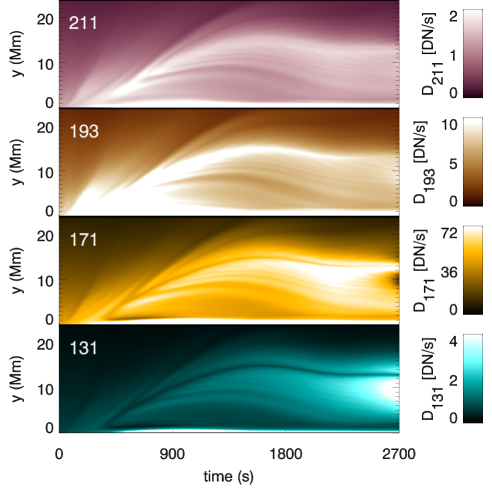
Figure 11: Time evolution of synthetic EUV emission through the 211$\mathrm{\AA}$, 193$\mathrm{\AA}$, 171$\mathrm{\AA}$, and 131$\mathrm{\AA}$ channels of AIA. $\log T_{\mathrm{peak}}$ = 6.2, 6.1, 5.8, and 5.6, respectively, where $T_{\mathrm{peak}}$ is the peak temperature of each channel. $l_{z}$ in Eq. (32) is set to 10 Mm. The emission is averaged in the area of $x<3\mathrm{Mm}$.

Figure 12: Relationship between $\mathrm{T_{c}}$ and maximum density. The modeled cases are indicated by letters. The solid line is the result of applying the scaling formula Eq. (33).

6 Conclusion

We proposed a new in-situ formation model of inverse-polarity prominence. The model was demonstrated in 2.5-dimensional MHD simulations, involving thermal conduction and radiative cooling. Either flux rope formation by anti-shearing motion or a heating model proportional to the local density is necessary for a in-situ prominence formation. From the results of a parameter study on cutoff temperature, we derived an empirical scaling formula that related the density of the prominences to their temperature. Our study quantitatively demonstrated that our in-situ formation model can reproduce the observed density of prominences. The study also explained the observed intensity shift among multi-wavelength EUV emission of in-situ condensation.

References

- Amari et al. (2003) Amari, T., Luciani, J. F., Aly, J. J., Mikic, Z., & Linker, J. 2003, ApJ, 585, 1073
- Antiochos et al. (1999) Antiochos, S. K., MacNeice, P. J., Spicer, D. S., & Klimchuk, J. A. 1999, ApJ, 512, 985
- Berger et al. (2012) Berger, T. E., Liu, W., & Low, B. C. 2012, ApJ, 758, L37
- Chen & Shibata (2000) Chen, P. F., & Shibata, K. 2000, ApJ, 545, 524
- Choe & Lee (1992) Choe, G. S., & Lee, L. C. 1992, Sol. Phys., 138, 291
- Fan & Gibson (2007) Fan, Y., & Gibson, S. E. 2007, ApJ, 668, 1232
- Hildner (1974) Hildner, E. 1974, Sol. Phys., 35, 123
- Hillier & van Ballegooijen (2013) Hillier, A., & van Ballegooijen, A. 2013, ApJ, 766, 126
- Kaneko & Yokoyama (2014) Kaneko, T., & Yokoyama, T. 2014, ApJ, 796, 44
- Karpen et al. (2006) Karpen, J. T., Antiochos, S. K., & Klimchuk, J. A. 2006, ApJ, 637, 531
- Keppens & Xia (2014) Keppens, R., & Xia, C. 2014, ApJ, 789, 22
- Kippenhahn & Schlüter (1957) Kippenhahn, R., & Schlüter, A. 1957, ZAp, 43, 36
- Kliem et al. (2004) Kliem, B., Titov, V. S., & Török, T. 2004, A&A, 413, L23
- Kliem & Török (2006) Kliem, B., & Török, T. 2006, Physical Review Letters, 96, 255002
- Koyama & Inutsuka (2004) Koyama, H., & Inutsuka, S.-i. 2004, ApJ, 602, L25
- Kudoh et al. (1999) Kudoh, T., Shibata, K., & Matsumoto, R. 1999, in Astrophysics and Space Science Library, Vol. 240, Numerical Astrophysics, ed. S. M. Miyama, K. Tomisaka, & T. Hanawa, 203
- Kuperus & Raadu (1974) Kuperus, M., & Raadu, M. A. 1974, A&A, 31, 189
- Kusano (2002) Kusano, K. 2002, ApJ, 571, 532
- Kusano et al. (2004) Kusano, K., Maeshiro, T., Yokoyama, T., & Sakurai, T. 2004, ApJ, 610, 537
- Leroy et al. (1984) Leroy, J. L., Bommier, V., & Sahal-Brechot, S. 1984, A&A, 131, 33
- Linker et al. (2001) Linker, J. A., Lionello, R., Mikić, Z., & Amari, T. 2001, J. Geophys. Res., 106, 25165
- Liu et al. (2012) Liu, W., Berger, T. E., & Low, B. C. 2012, ApJ, 745, L21
- Low et al. (2012a) Low, B. C., Berger, T., Casini, R., & Liu, W. 2012a, ApJ, 755, 34
- Low et al. (2012b) Low, B. C., Liu, W., Berger, T., & Casini, R. 2012b, ApJ, 757, 21
- Luna et al. (2012) Luna, M., Karpen, J. T., & DeVore, C. R. 2012, ApJ, 746, 30
- Mackay et al. (2010) Mackay, D. H., Karpen, J. T., Ballester, J. L., Schmieder, B., & Aulanier, G. 2010, Space Sci. Rev., 151, 333
- Martens & Zwaan (2001) Martens, P. C., & Zwaan, C. 2001, ApJ, 558, 872
- Sharma & Hammett (2007) Sharma, P., & Hammett, G. W. 2007, Journal of Computational Physics, 227, 123
- Shiota et al. (2005) Shiota, D., Isobe, H., Chen, P. F., et al. 2005, ApJ, 634, 663
- Török & Kliem (2005) Török, T., & Kliem, B. 2005, ApJ, 630, L97
- van Ballegooijen & Martens (1989) van Ballegooijen, A. A., & Martens, P. C. H. 1989, ApJ, 343, 971
- Xia et al. (2012) Xia, C., Chen, P. F., & Keppens, R. 2012, ApJ, 748, L26
- Xia et al. (2014a) Xia, C., Keppens, R., Antolin, P., & Porth, O. 2014a, ApJ, 792, L38
- Xia et al. (2014b) Xia, C., Keppens, R., & Guo, Y. 2014b, ApJ, 780, 130
- Xiao et al. (1996) Xiao, F., Yabe, T., Nizam, G., & Ito, T. 1996, Computer Physics Communications, 94, 103
- Yokoyama & Shibata (1994) Yokoyama, T., & Shibata, K. 1994, ApJ, 436, L197