Multiuser Wireless Power Transfer via Magnetic Resonant Coupling: Performance Analysis, Charging Control, and Power Region Characterization

Abstract

Magnetic resonant coupling (MRC) is an efficient method for realizing the near-field wireless power transfer (WPT). Although the MRC enabled WPT (MRC-WPT) with a single pair of transmitter and receiver has been thoroughly studied in the literature, there is limited work on the general setup with multiple transmitters and/or receivers. In this paper, we consider a point-to-multipoint MRC-WPT system with one transmitter delivering wireless power to a set of distributed receivers. We aim to introduce new applications of signal processing and optimization techniques to the performance characterization and optimization in multiuser WPT via MRC. We first derive closed-form expressions for the power drawn from the energy source at the transmitter and that delivered to the load at each receiver. We identify a “near-far” fairness issue in multiuser power transmission due to receivers’ distance-dependent mutual inductance with the transmitter. To tackle this issue, we propose a centralized charging control algorithm to jointly optimize the receivers’ load resistance to minimize the total transmitter power drawn while meeting the given power requirement of each individual load. For ease of practical implementation, we also devise a distributed algorithm for the receivers to adjust their load resistance independently in an iterative manner. Last, we characterize the power region that constitutes all the achievable power-tuples of the loads via controlling their adjustable resistance. In particular, we compare the power regions without versus with the time sharing of users’ power transmission, where it is shown that time sharing yields a larger power region in general. Extensive simulation results are provided to validate our analysis and corroborate our study on the multiuser MRC-WPT system.

I Introduction

Inductive coupling [2, 3] is a traditional method to realize the near-field wireless power transfer (WPT) for short-range applications in e.g., centimeters. Recently, magnetic resonant coupling (MRC) [4, 5, 6, 7] has drawn significant interest for implementing the near-field WPT due to its high power transfer efficiency as well as long operation range, say, up to a couple of meters. Furthermore, MRC effectively avoids the power leakage to non-resonant externalities and thus ensures safety to the neighboring environment.

Two different methods are commonly adopted in practice to implement MRC enabled WPT (MRC-WPT). In the first method [4, 5], resonators, each of which is a tunable RLC circuit, are placed in close proximity of the electromagnetic (EM) coils of the energy transmitters and receivers to efficiently transfer power between them. Since resonators are designed to resonate at the system’s operating frequency, the total reactive power consumption in the system is effectively minimized at resonance and hence high power transfer efficiency is achieved over longer distance as compared to conventional inductive coupling. In the second method [6, 7], series and/or shunt compensators, each of which is a capacitor of variable capacity, are embedded in the electric circuits of energy transmitters and receivers with their natural frequencies set same as the system’s operating frequency to achieve resonance. Generally speaking, the second method achieves higher power transfer efficiency over the first method, since in the first method resonators incur additional power loss due to their parasitic resistance. However, the electric circuits of energy transmitters and receivers need to be accessible in the second method to embed compensators in them.

The MRC-WPT system with a single pair of transmitter and receiver has been extensively studied in the literature, with the aims such as maximizing the end-to-end power transfer efficiency or maximizing the power delivered to the receiver’s load with a given input power [8, 9, 10, 11]. Moreover, systems with two transmitters and a single receiver or with a single transmitter and two receivers have been studied in [12, 13, 14, 15, 16], while their results cannot be directly applied to the systems with more than two transmitters/receivers. Recently, an MRC-WPT system with multiple transmitters and one single receiver has been investigated in [17] to wirelessly charge a cellphone located at $40$ centimeters away, independent of the phone’s orientation. However, the interactions between the energy transmitters and receiver were demonstrated only through simulations in [17]. There have been other recent works (see e.g. [18, 19]) on optimizing the performance of MRC-WPT systems with multiple transmitters and one single receiver.

Different from the above works, in this paper we consider a point-to-multipoint MRC-WPT system based on the series compensator method aforementioned, as shown in Fig. 1, where one transmitter that is connected to a stable energy source supplies wireless power to a set of distributed receivers. Each receiver is connected to an electric load via a switch, where the switch connects/disconnects the load to/from the receiver.

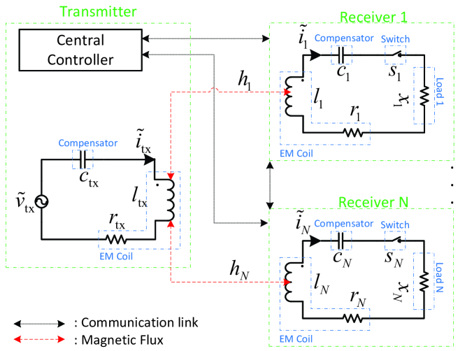
Figure 1: A point-to-multipoint magnetic resonant coupling enabled wireless power transfer system with communication and control.

We aim to apply signal processing and optimization techniques to the performance characterization and optimization in multiuser MRC-WPT systems. First, by extending the results in [12, 13, 14, 15, 16, 17], we derive closed-form expressions for the power drawn from the energy source at the transmitter and that delivered to the load at each receiver, in terms of mutual inductance among the transmitter and receivers as well as their circuit parameters, for arbitrary number of receivers. Our obtained results reveal a near-far fairness issue in multiuser wireless power transmission, similar to its counterpart phenomenon in multiuser wireless communication. Specifically, a receiver that is far from the transmitter and thus has a small mutual inductance with the transmitter receives lower power as compared to a receiver that is closer to the transmitter, with other circuit parameters given identical. Next, we propose a method to mitigate the near-far issue by jointly designing the load resistance of all receivers to control their received power by exploiting the mutual coupling effect in the MRC-WPT system. This is analogous and yet in sharp contrast to the method of adjusting antenna weights at the transmitter to control the received power at different receivers in the existing far-field microwave or radio frequency (RF) transmission enabled WPT [20, 21].

In particular, we consider the scenario where a central controller is equipped at the transmitter to coordinate the multiuser power charging, by assuming that it has the full knowledge of all receivers, including their circuit parameters and power requirements. The central controller jointly designs the adjustable load resistance of all receivers to minimize the total power consumed at the transmitter subject to the given minimum power requirement of each load. For ease of practical implementation, we also consider the scenario without any central controller installed and devise a distributed algorithm for multiuser charging control by adjusting the loads’ resistance at their individual receivers in an iterative manner. In our proposed distributed algorithm, each receiver sets its load resistance independently based on its local information and a one-bit feedback broadcasted by each of the other receivers. The feedback of each receiver indicates whether the received power of its load exceeds the required minimum power level or not. It is shown via simulations that the distributed algorithm achieves performance fairly close to the optimal solution by the centralized algorithm with a finite number of iterations.

Last, we characterize the power region for multiuser power transfer which constitutes all the achievable power-tuples for the receiver loads via controlling their adjustable resistance in given ranges. Specifically, we introduce the time-sharing based multiuser power transfer, where the transmission is divided into orthogonal time slots and within each time slot only a selected subset of receivers are scheduled to receive power, while the other receivers are disconnected from their loads. This is aimed to more flexibly control the mutual coupling effect between the transmitter and receivers in WPT. It is shown that time sharing can enlarge the power region over the case without time sharing in general. It is also shown that time sharing can further mitigate the near-fare issue in multiuser WPT by allocating more time to receivers that are more far-away from the transmitter. Furthermore, we extend the centralized multiuser charging control algorithm for the case without time sharing to jointly optimize the time allocation and load resistance for all the receivers in the case with time sharing, to further reduce the transmitter power consumption under the same average power requirement of each load.

The rest of this paper is organized as follows. Section II introduces the system model. Section III presents our analytical results. Section IV presents both the centralized and distributed multiuser power charging control algorithms. Section V characterizes and compares the power regions without versus with time sharing. Finally, we conclude the paper in Section VI.

II System model

As shown in Fig. 1, we consider an MRC-WPT system with a single transmitter and $N\geq 1$ receivers, indexed by $n$, $n\in{\cal N}=\{1,\ldots,N\}$. The transmitter and receivers are equipped with EM coils for realizing wireless power transfer, while an embedded communication system is assumed to enable information exchange among them. The transmitter is connected to a stable energy source supplying sinusoidal voltage over time given by $\tilde{v}_{\text{tx}}(t)=\text{Re}\{{v}_{\text{tx}}e^{jwt}\}$, with ${v}_{\text{tx}}$ denoting a complex voltage which is assumed to be constant, and $w>0$ denoting its operating angular frequency. Each receiver $n$ is connected via a switch to a given electric load (e.g., battery charger), named load $n$, with adjustable resistance $x_{n}>0$. The switch is used to connect/disconnect each load to/from its corresponding receiver. The state of switch at each receiver $n$ is given by $s_{n}\in\{0,~{}1\}$, where $s_{n}=1$ and $s_{n}=0$ denote the switch is closed and open, respectively. It is also assumed that the transmitter and each receiver $n$ are compensated using series capacitors with capacities $c_{\text{tx}}>0$ and $c_{n}>0$, respectively.

Let $\tilde{i}_{\text{tx}}(t)=\text{Re}\{i_{\text{tx}}e^{jwt}\}$, with complex-valued ${i}_{\text{tx}}$, denote the steady state current flowing through the transmitter. This current produces a time-varying magnetic flux in the transmitter’s EM coil, which passes through the EM coils of nearby receivers and induces time-varying currents in them. We denote $\tilde{i}_{n}(t)=\text{Re}\{i_{n}e^{jwt}\}$, with complex-valued ${i}_{n}$, as the steady state current at receiver $n$. It is worth pointing out that the magnetic flux is the main medium of wireless power transfer considered in this paper, while the electric field is evanescent and thus is ignored [4]. This is in contrast to the RF based far-field WPT [20, 21], where the synchronized oscillations of magnetic and electric fields radiate energy in the form of EM waves propagating through the air.

We denote $r_{\text{tx}}>0$ ($r_{n}>0$) and $l_{\text{tx}}>0$ ($l_{n}>0$) as the internal resistance and the self-inductance of the EM coil of the transmitter (receiver $n$), respectively. We also denote the mutual inductance between EM coils of the transmitter and each receiver $n$ by a real number $h_{n}$, with $|h_{n}|\leq\sqrt{l_{n}l_{\text{tx}}}$, where its actual value depends on the physical characteristics of the two EM coils, their locations, alignment (or misalignment) of oriented axes with respect to each other, the environment magnetic permeability, etc. For example, the mutual inductance of two coaxial circular loops that lie in the parallel planes with separating distance of $d$ meter is shown to be proportional to $d^{-3}$ in [23]. Moreover, since the receivers usually employ smaller EM coils than that of the transmitter due to practical size limitation and they are also physically separated, we ignore the mutual inductance between any pair of the receivers for simplicity.

The equivalent electric circuit model of the considered MRC-WPT system is also shown in Fig. 1, in which the natural angular frequencies of the transmitter and each receiver $n$ can be expressed as $w_{\text{natural},\text{tx}}={1}/{\sqrt{l_{\text{tx}}c_{\text{tx}}}}$ and $w_{\text{natural},n}={1}/{\sqrt{l_{n}c_{n}}}$, respectively. We thus set the capacities of compensators’ capacitors as

$$c_{\text{tx}} =\dfrac{1}{l_{\text{tx}}\hskip 1.70717ptw^{2}},$$ (1)

$$c_{n} =\dfrac{1}{l_{n}\hskip 1.70717ptw^{2}},~{}\forall n\in\cal N,$$ (2)

so that the transmitter and all receivers have the same natural angular frequency as the transmitter voltage source’s angular frequency $w$, i.e., $w_{\text{natural},\text{tx}}=w_{\text{natural},1}=\ldots=w_{\text{natural},N}=w$. Accordingly, we name $w$ as the resonant angular frequency.

In this paper, we assume that the transmitter and all receivers are at fixed positions and the physical characteristics of their EM coils are a priori known. As a result, $h_{n}$’s, $\forall n\in\cal N$, are modeled as given constants, which are computed according to Appendix E. In practical systems with mobile receivers, $h_{n}$’s in general change over time and thus need to be measured periodically. For example, one method that can be used in practice to estimate the mutual inductance between the transmitter and any receiver $n$, is given as follows. First, by disconnecting the loads at all other receivers $k\neq n$, under a known input voltage $v_{\text{tx}}$, the transmitter measures the power drawn from its voltage source, denoted by $p_{\text{tx}}$, due to load $n$ only. From (8), we can show

$$h_{n}=\pm\dfrac{\sqrt{\left(\dfrac{|v_{\text{tx}}|^{2}}{2p_{\text{tx}}}-r_{\text{tx}}\right)\left(r_{n}+x_{n}\right)}}{w},$$ (3)

i.e., the transmitter can obtain the mutual inductance with receiver $n$ by assuming known $r_{n}$ and $x_{n}$ (which can be sent to the transmitter via one-time feedback from receiver $n$). Note that the sign of $h_{n}$ can be determined by comparing the known direction of the current flowing in receiver $n$ (via a one-bit feedback from receiver $n$) with that assumed at the transmitter. If the directions are same, then the positive sign is selected for $h_{n}$; otherwise, the negative sign is set.

In this paper, we treat the load resistance $x_{n}$’s, $\forall n\in\cal N$, as design parameters, which can be adjusted in real time to control the performance of our considered MRC-WPT system based on the information shared among different nodes in the system, via the embedded communication system. Note that an electric load with any fixed resistance can be connected via a rectifier in parallel with a boost (or triboost) converter to each receiver to realize an adjustable resistance [24]. Specifically, given the fixed input voltage, the on/off time intervals of the converter can be controlled in real time to change the average current flowing into the load, which is equivalent to adjusting the load resistance.

III Performance Analysis

In this section, we present new analytical results on the performance of the MRC-WPT system with arbitrary number of receivers. A numerical example is also provided to validate our analysis and draw useful insights. Here, we assume that all receiver switches are closed, i.e., $s_{n}=1$, $\forall n\in\cal N$; as a result, the transmitter sends wireless power to all loads concurrently.

III-A Analytical Results

By applying Kirchhoff’s circuit laws to the electric circuit model given in Fig. 1, we have

$$\left(r_{\text{tx}}+j\left(wl_{\text{tx}}-\dfrac{1}{wc_{\text{tx}}}\right)\right)i_{\text{tx}}-jw\sum_{k\in\cal N}h_{k}i_{k} =v_{\text{tx}},$$ (4)

$$\left(r_{n}+x_{n}+j\left(wl_{n}-\dfrac{1}{wc_{n}}\right)\right)i_{n}-jwh_{n}i_{\text{tx}} =0,~{}\forall n\in\cal N.$$ (5)

From (1) and (2), we can set $wl_{\text{tx}}-{1}/{(wc_{\text{tx}})}=0$ and $wl_{n}-{1}/{(wc_{n})}=0$ in (4) and (5), respectively. This is due to the fact that the transmitter and all receivers are designed to resonate at the same angular frequency $w$. By solving the set of linear equations given in (4) and (5), we can derive $i_{\text{tx}}$ and $i_{n}$’s as functions of the input voltage $v_{\text{tx}}$ as follows:

$$i_{\text{tx}} =~{}\dfrac{1}{r_{\text{tx}}+w^{2}\sum_{k\in\cal N}h_{k}^{2}\left(r_{k}+x_{k}\right)^{-1}}v_{\text{tx}},$$ (6)

$$i_{n} =j\dfrac{wh_{n}\left(r_{n}+x_{n}\right)^{-1}}{r_{\text{tx}}+w^{2}\sum_{k\in\cal N}h_{k}^{2}\left(r_{k}+x_{k}\right)^{-1}}v_{\text{tx}},~{}\forall n\in\cal N.$$ (7)

The power drawn from the energy source at the transmitter, i.e., $p_{\text{tx}}$, and that delivered to each load $n$, denoted by $p_{n}$, are then obtained as

$$p_{\text{tx}} =\dfrac{1}{2}\text{Re}\left\{v_{\text{tx}}i_{\text{tx}}^{*}\right\}=\dfrac{|v_{\text{tx}}|^{2}}{2}\dfrac{1}{r_{\text{tx}}+w^{2}\sum_{k\in\cal N}h_{k}^{2}\left(r_{k}+x_{k}\right)^{-1}},$$ (8)

$$p_{n} =\dfrac{1}{2}x_{n}\left|i_{n}\right|^{2}=\dfrac{|v_{\text{tx}}|^{2}}{2}\dfrac{w^{2}h_{n}^{2}x_{n}\left(r_{n}+x_{n}\right)^{-2}}{\left(r_{\text{tx}}+w^{2}\sum_{k\in\cal N}h_{k}^{2}\left(r_{k}+x_{k}\right)^{-1}\right)^{2}},$$ (9)

where $i_{\text{tx}}^{*}$ denotes the conjugate of $i_{\text{tx}}$. From (9), it follows that the power delivered to each load $n$ increases with the mutual inductance between EM coils of its receiver and the transmitter, i.e., $h_{n}$. This can cause a near-far fairness issue since a receiver that is far from the transmitter generally has a small mutual inductance with the transmitter; as a result, its received power is lower than that at a receiver that is closer to the transmitter (thus has a larger mutual inductance). Furthermore, we define $p_{\text{sum}}=\sum_{k=1}^{N}p_{k}$ as the sum-power delivered to all loads, where it can be verified from (8) and (9) that $p_{\text{sum}}<p_{\text{tx}}$. The sum-power transfer efficiency, denoted by $0\leq\rho<1$, is thus expressed as

$$\rho=\dfrac{p_{\text{sum}}}{p_{\text{tx}}}=\dfrac{w^{2}\sum_{k\in\cal N}h_{k}^{2}\hskip 0.85358ptx_{k}\hskip 0.85358pt\left(r_{k}+x_{k}\right)^{-2}}{r_{\text{tx}}+w^{2}\sum_{k\in\cal N}h_{k}^{2}\left(r_{k}+x_{k}\right)^{-1}}.$$ (10)

Remark III.1

When the receivers are all weakly coupled to the transmitter, e.g., they are sufficiently far away from the transmitter, we have $h_{n}\rightarrow 0$, $\forall n\in\cal N$. In this regime, from (8), it follows that the transmitter power is $p_{\text{tx}}\approx|v_{\text{tx}}|^{2}/(2r_{\text{tx}})$, which is a function of the resistance and voltage of the transmitter only. On the other hand, from (9), it follows that the power delivered to each load $n$ is $p_{n}\approx|v_{\text{tx}}|^{2}w^{2}h_{n}^{2}x_{n}(r_{n}+x_{n})^{-2}/(2r_{\text{tx}}^{2})$, which is irrespective of the other receivers’ mutual inductance and resistance. The above results can be explained as follows. With $h_{n}\rightarrow 0$, $\forall n\in\cal N$, the power transfered to the receivers is small and thus can be neglected as compare to the power loss due to the transmitter’s resistance. As a result, we have $p_{\text{tx}}\approx r_{\text{tx}}|i_{\text{tx}}|^{2}/2$, with $i_{\text{tx}}=v_{\text{tx}}/r_{\text{tx}}$. It also can be verified that with $h_{n}\rightarrow 0$, $\forall n\in\cal N$, the coupling effect among the receivers through the transmitter current $i_{\text{tx}}$ is negligible. Hence, the power delivered to the load at each receiver is independent of other receivers (similar to the far-field RF based WPT [20, 21]).

Remark III.2

It can be shown from (9) that $p_{n}$, $\forall n\in\cal N$, first increases over $0<w<\dot{w}$, and then decreases over $w>\dot{w}$, where

$$\dot{w}=\sqrt{\dfrac{r_{\text{tx}}}{\sum_{k\in\cal N}h_{k}^{2}\left(r_{k}+x_{k}\right)^{-1}}}.$$ (11)

The above result can be explained as follows. From (7), it follows that the magnitude of the current flowing in each receiver $n$, i.e., $|i_{n}|$, strictly increases over $0<w<\dot{w}$, but strictly decreases over $w>\dot{w}$. This yields that $w=\dot{w}$ is the unique maximizer of $|i_{n}|$ over $w>0$. Obviously, $p_{n}$, which is defined in (9) as $p_{n}=x_{n}|i_{n}|^{2}/2$, behaves same as $|i_{n}|$ over $w>0$. Although $w$ is assumed to be fixed in this paper, it can also be optimally set to maximize the system power transfer efficiency, if this is implementable in practice. Furthermore, from (11), it follows that $\dot{w}$ depends on the distances between the transmitter and receivers, since $h_{n}$’s in general decrease with larger distances.

Next, we study the effect of changing the load resistance of one particular receiver $n$, i.e., $x_{n}$, on the transmitter power $p_{\text{tx}}$, its received power $p_{n}$, the power delivered to each of the other loads $m\in\cal N$, $m\neq n$, i.e., $p_{m}$, the sum-power delivered to all loads $p_{\text{sum}}$, and the sum-power transfer efficiency $\rho$, assuming that all the other loads’ resistance is fixed.

Proposition III.1

$p_{\textnormal{tx}}$ strictly increases over $x_{n}>0$.

Proof:

Please see Appendix A. ∎

This result can be explained as follows. From (6), it is observed that the transmitter current $|i_{\text{tx}}|$ strictly increases over $x_{n}>0$. Since the energy source voltage $v_{\text{tx}}$ is fixed, it follows that $p_{\text{tx}}$ given in (8) strictly increases over $x_{n}>0$.

Proposition III.2

$p_{m}$, $\forall m\neq n$, strictly increases over $x_{n}>0$. However, $p_{n}$ first increases over $0<x_{n}<\dot{x}_{n}$, and then decreases over $x_{n}>\dot{x}_{n}$, where

$$\dot{x}_{n}=\dfrac{r_{n}\left(r_{\textnormal{tx}}+\phi_{n}\right)+w^{2}h_{n}^{2}}{r_{\textnormal{tx}}+\phi_{n}},$$ (12)

with $\phi_{n}=w^{2}\sum_{k\in{\cal N}\setminus\{n\}}h_{k}^{2}(r_{k}+x_{k})^{-1}$.

Proof:

Please see Appendix B. ∎

The above result can be explained as follows. From (7), it follows that for each receiver $m$, $m\neq n$, its current $|i_{m}|$ strictly increases over $x_{n}>0$. The received power $p_{m}$ defined in (9) thus strictly increases over $x_{n}>0$. On the other hand, it follows from (7) that for receiver $n$, its current $|i_{n}|$ strictly decreases over $x_{n}>0$. However, from (9), it follows that the decrement in $|i_{n}|^{2}$ is smaller than the increment of $x_{n}$ when $0<x_{n}<\dot{x}_{n}$; therefore, $p_{n}$ increases over $x_{n}$ in this region. The opposite is true when $x_{n}>\dot{x}_{n}$.

Proposition III.3

If $r_{\textnormal{tx}}+\phi_{n}-2\varphi_{n}\leq 0$, $p_{\textnormal{sum}}$ strictly increases over $x_{n}>0$, where $\varphi_{n}=w^{2}\sum_{k\in{\cal N}\setminus\{n\}}h_{k}^{2}x_{k}(r_{k}+x_{k})^{-2}$; otherwise, $p_{\textnormal{sum}}$ first increases over $0<x_{n}<\ddot{x}_{n}$, and then decreases over $x_{n}>\ddot{x}_{n}$, where

$$\ddot{x}_{n}=\dfrac{r_{n}\left(r_{\textnormal{tx}}+\phi_{n}\right)+w^{2}h_{n}^{2}+2r_{n}\varphi_{n}}{r_{\textnormal{tx}}+\phi_{n}-2\varphi_{n}}.$$ (13)

Proof:

Please see Appendix C. ∎

This result is a consequence of Proposition III.2, from which it is known that $p_{m}$’s, $m\neq n$, strictly increase over $x_{n}>0$, while $p_{n}$ first increases over $0<x_{n}<\dot{x}_{n}$ and then decreases over $x_{n}>\dot{x}_{n}$. The sum-power $p_{\text{sum}}$ can thus behave similarly as either $p_{m}$’s (monotonically increasing) or $p_{n}$ (initially increasing and then decreasing) over $x_{n}>0$, depending on the system parameters.

Proposition III.4

If $\varphi_{n}-\phi_{n}-r_{\text{tx}}\geq 0$, $\rho$ strictly increases over $x_{n}>0$; otherwise, $\rho$ first increases over $0<x_{n}<\dddot{x}_{n}$, and then decreases over $x_{n}>\dddot{x}$, where

$$\dddot{x}=\dfrac{-r_{n}\varphi_{n}-\sqrt{r_{n}^{2}\varphi_{n}^{2}-\Gamma_{n}}}{\varphi_{n}-\phi_{n}-r_{\text{tx}}},$$ (14)

with $\Gamma_{n}=(\varphi_{n}-\phi_{n}-r_{\text{tx}})(r_{n}^{2}(r_{\text{tx}}+\varphi_{n}+\phi_{n})+r_{n}w^{2}h_{n}^{2})$.

Proof:

Please see Appendix D. ∎

This result is a consequence of Propositions III.1 and III.3, due to the different behaviors of $p_{\text{tx}}$ and $p_{\text{sum}}$ over $x_{n}>0$.

III-B Validation of Analysis

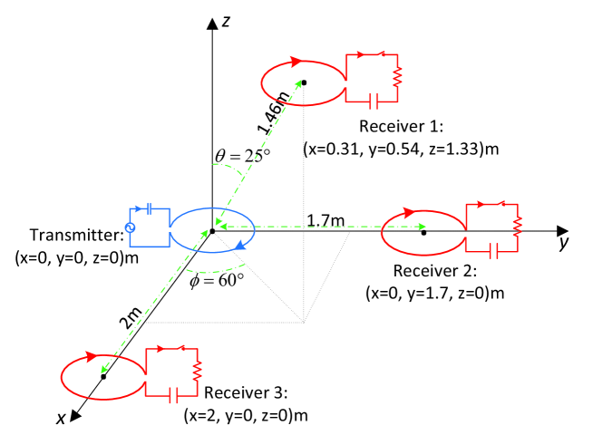
Figure 2: The considered system setup for numerical examples.

For the purpose of exposition, we consider a point-to-multipoint MRC-WPT system with $N=3$ receivers, as shown in Fig. 2, where the transmitter and receivers use circular EM coils (see Fig. 12 in Appendix -E), with the physical characteristics given in Table I. Note that the transmitter and both receivers $2$ and $3$ lie in the plane with $z=0$, while receiver $1$ lies in the plane with $z=0.91$ meter (m). Accordingly, the internal resistance and self-inductance of individual EM coils as well as the mutual inductance among them can be derived (see the details in Appendix -E), where the obtained values are given in Table II. In this example, although all receivers use EM coils with the same physical characteristics, they are located in different distances from the transmitter. Specifically, receiver $1$ is closest to the transmitter and thus has the largest mutual inductance with the transmitter, while receiver $3$ is farthest and has the smallest mutual inductance.

TABLE I: Physical characteristics of EM coils

EM Coil	Inner radius (cm)	Outer radius (cm)	Average radius (cm)	Number of turns	Material of wire	Resistivity of wire ($\mu\Omega$/m)
Transmitter	$19.9$	$20.1$	$20$	$200$	Copper	$0.0168$
Receiver $1$	$4.95$	$5.05$	$5$	$10$	Copper	$0.0168$
Receiver $2$	$4.95$	$5.05$	$5$	$10$	Copper	$0.0168$
Receiver $3$	$4.95$	$5.05$	$5$	$10$	Copper	$0.0168$

TABLE II: Electrical characteristics of EM coils

EM Coil	Internal resistance $r_{\text{tx}}$/$r_{n}$ ($\Omega$)	Self-inductance $l_{\text{tx}}$/$l_{n}$ (mH)	Mutual inductance $h_{n}$ ($\mu$H)
Transmitter	$1.3440$	$54.0630$	–
Receiver $1$	$0.0672$	$0.0294$	$-0.0921$
Receiver $2$	$0.0672$	$0.0294$	$~{}0.0402$
Receiver $3$	$0.0672$	$0.0294$	$~{}0.0245$

We set $v_{\text{tx}}=20\sqrt{2}$V, and $w=42.6\times 10^{6}$rad/s (i.e., $6.78$MHz), as suggested in the A4WP specification [22]. For this example, we fix $x_{2}=x_{3}=2.5\Omega$.

First, we plot $p_{\text{tx}}$, $p_{n}$’s, $\forall n\in\cal N$, and $p_{\text{sum}}$ versus the resistance of load $1$, i.e., $x_{1}$, in Fig. 3. It is observed that $p_{\text{tx}}$, $p_{2}$, $p_{3}$ and $p_{\text{sum}}$ all increase over $x_{1}>0$; however, $p_{1}$ initially increases over $0<x_{1}<\dot{x}_{1}=5.35\Omega$ and then declines over $x_{1}>5.35\Omega$. Note that in this example, the condition $r_{\textnormal{tx}}+\phi_{n}-2\varphi_{n}<0$ holds in Proposition III.3. The obtained results are all consistent with our analysis in Section III-A. Besides, we observe that varying $x_{1}$ not only changes $p_{1}$, but also the power delivered to other loads. For instance, receiver $1$ can help receivers $2$ and $3$, which are farther away from the transmitter, to receive more power by increasing its load resistance $x_{1}$. This is a useful mechanism that will be utilized later in this paper to mitigate the near-far issue.

Second, in Fig. 4, we plot the sum-power transfer efficiency $\rho$ as a function of $x_{1}$. It is observed that $\rho$ follows a single-peak pattern over $x_{n}>0$, i.e., it first increases over $0<x_{1}<\dddot{x}_{1}=0.95\Omega$, and then smoothly declines over $x_{1}>0.95\Omega$. This result can be verified from Proposition III.4 by considering the fact that in this example, the condition $\varphi_{n}-\phi_{n}-r_{\text{tx}}<0$ holds. Note that when $x_{1}\rightarrow\infty$, it follows from (6) and (8) that $i_{1}\rightarrow 0$ and $p_{1}\rightarrow 0$. This is equivalent to disconnecting load $1$ from receiver $1$, i.e., setting $s_{1}=0$. As a result, the efficiency converges when $x_{1}\rightarrow\infty$, while the converged value depends on the parameters of the transmitter and the other two receivers.

Third, we set $x_{1}=x_{2}=x_{3}=2.5\Omega$, and plot the power received by the three loads versus $w$ in Fig. 5. It is observed that $p_{1}$, $p_{2}$, and $p_{3}$ reach their individual peaks all at $w=\dot{w}=17.97\times 10^{6}$rad/sec, which is in accordance to Remark III.2. It is worth noting that although $w$ and $x_{n}$’s can be jointly designed to achieve better performance over the case of optimizing $x_{n}$’s only with $w$ being fixed, this problem is challenging to solve and thus is left as our future work.

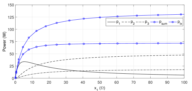
Figure 3: Input and output power versus $x_{1}$.

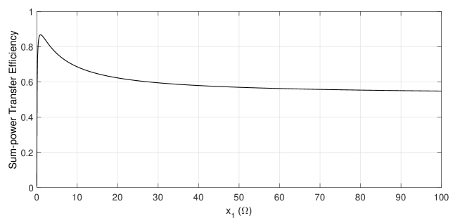
Figure 4: The sum-power transfer efficiency $\rho$ versus $x_{1}$.

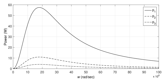
Figure 5: The output power versus $w$.

IV Multiuser Charging Control Optimization

In this section, we optimize the receivers’ load resistance $x_{n}$’s to minimize the transmitter power $p_{\text{tx}}$ subject to the given load constraints, by assuming that $s_{n}=1$, $\forall n\in\cal N$, i.e., all the receives are connected to their loads. First, we consider the case with a central controller at the transmitter, which has the full knowledge of all receivers, including their circuit parameters as well as their load requirements, to implement centralized charging control. We then devise a distributed charging algorithm for the receivers to independently adjust their load resistance iteratively, for the ease of practical implementation. Last, we compare the performance of the two algorithms under a practical system setup.

IV-A Problem Formulation

We assume that in practice the resistance of each load $n$ can be adjusted over a given range $\underline{x}_{n}\leq x_{n}\leq\overline{x}_{n}$, where $\underline{x}_{n}>0$ ($\overline{x}_{n}\geq\underline{x}_{n}$) is the lower (upper) limit of the resistance. It is also assumed that the power delivered to each load $n$ needs to be higher than a given minimum threshold $\underline{p}_{n}>0$ to guarantee its quality of service. Next, we formulate the optimization problem (P1) to minimize the transmitter power $p_{\text{tx}}$ subject to the given load constraints of all receivers as follows.

$$\mathrm{(P1)}:\mathop{\mathtt{min}}_{\{\underline{x}_{n}\leq x_{n}\leq\overline{x}_{n}\}_{n\in\cal N}} ~{}\dfrac{|v_{\text{tx}}|^{2}}{2}\dfrac{1}{r_{\text{tx}}+w^{2}\sum_{k\in\cal N}h_{k}^{2}\left(r_{k}+x_{k}\right)^{-1}}$$ (15)

$$\mathtt{s.t.} ~{}\dfrac{|v_{\text{tx}}|^{2}}{2}\dfrac{w^{2}h_{n}^{2}x_{n}\left(r_{n}+x_{n}\right)^{-2}}{\left(r_{\text{tx}}+w^{2}\sum_{k\in\cal N}h_{k}^{2}\left(r_{k}+x_{k}\right)^{-1}\right)^{2}}\geq\underline{p}_{n},\forall n\in\cal N.$$ (16)

Although (P1) is non-convex, we propose a centralized algorithm to solve it optimally in the next subsection.

IV-B Centralized Algorithm

First, based on (P1), we formulate the maximization problem (P2), where its objective function is the inverse of that of (P1) but with the same constraints as (P1).

$$\mathrm{(P2)}:\mathop{\mathtt{max}}_{\{\underline{x}_{n}\leq x_{n}\leq\overline{x}_{n}\}_{n\in\cal N}} ~{}\dfrac{2}{|v_{\text{tx}}|^{2}}\left(r_{\text{tx}}+w^{2}\sum_{k\in\cal N}h_{k}^{2}\left(r_{k}+x_{k}\right)^{-1}\right)$$ (17)

$$\mathtt{s.t.} ~{}\dfrac{|v_{\text{tx}}|^{2}}{2}\dfrac{w^{2}h_{n}^{2}x_{n}\left(r_{n}+x_{n}\right)^{-2}}{\left(r_{\text{tx}}+w^{2}\sum_{k\in\cal N}h_{k}^{2}\left(r_{k}+x_{k}\right)^{-1}\right)^{2}}\geq\underline{p}_{n},~{}\forall n\in\cal N.$$ (18)

It can be verified that the optimal solution to (P2) also solves (P1); as a result, we can equivalently solve (P2) to derive the optimal solution to (P1). Although (P2) is still non-convex, we can re-formulate it as a convex problem by applying change of variables. Specifically, we define a new set of variables as $y_{n}=1/(r_{n}+x_{n})$, $\forall n\in\cal N$. Since $\underline{x}_{n}\leq x_{n}\leq\overline{x}_{n}$, it follows that $\underline{y}_{n}\leq y_{n}\leq\overline{y}_{n}$, where $\underline{y}_{n}=1/(r_{n}+\overline{x}_{n})$ and $\overline{y}_{n}=1/(r_{n}+\underline{x}_{n})$. Accordingly, we rewrite (P2) as (P3).

$$\mathrm{(P3)}:\mathop{\mathtt{max}}_{\{\underline{y}_{n}\leq y_{n}\leq\overline{y}_{n}\}_{n\in\cal N}} ~{}\dfrac{2}{|v_{\text{tx}}|^{2}}{\left(r_{\text{tx}}+w^{2}\sum_{k\in\cal N}h_{k}^{2}\hskip 1.42262pty_{k}\right)}$$ (19)

$$\mathtt{s.t.} ~{}\dfrac{|v_{\text{tx}}|^{2}}{2}w^{2}h_{n}^{2}\left(r_{n}y_{n}^{2}-y_{n}\right)+\underline{p}_{n}\left(r_{\text{tx}}+w^{2}\sum_{k\in\cal N}h_{k}^{2}\hskip 1.42262pty_{k}\right)^{2}\leq 0,~{}\forall n\in\cal N.$$ (20)

Note that (P3) is a convex optimization problem, with a linear objective function and linear/quadratic inequality constraints over $y_{n}$’s. As a result, (P3) can be efficiently solved using the existing software, e.g., CVX [26]. Let $(y_{1}^{*},\ldots,y_{N}^{*})$ denote the optimal solution to (P3). The optimal solution to (P2) is thus obtained by a change of variable as $x_{n}^{*}=1/y_{n}^{*}-r_{n}$, $\forall n\in\cal N$. The obtained $(x_{1}^{*},\ldots,x_{N}^{*})$ also solves (P1). The centralized algorithm to solve (P1) is summarized in Table III, denoted as Algorithm $1$. Since the feasibility of convex problem (P3) can be efficiently checked, in the rest of this paper, we assume that (P1), or equivalently (P3), is feasible without loss of generality.

TABLE III: Centralized algorithm for (P1).

  Algorithm $1$  

• For each receiver $n$, $\forall n\in\cal N$, given $\underline{x}_{n}>0$ and $\overline{x}_{n}>\underline{x}_{n}$, compute $\underline{y}_{n}=1/(r_{n}+\overline{x}_{n})$ and $\overline{y}_{n}=1/(r_{n}+\underline{x}_{n})$. Accordingly, formulate the problem (P3).

• If (P3) is feasible, then save its optimal solution as $(y_{1}^{*},\ldots,y_{N}^{*})$. Set $x_{n}^{*}=1/y_{n}^{*}-r_{n}$, $\forall n\in\cal N$. Return $(x_{1}^{*},\ldots,x_{N}^{*})$ as the optimal solution to (P1).

• If (P3) is infeasible, then it follows that there is no feasible solution to (P1) and thus the algorithm terminates.

 

IV-C Distributed Algorithm

In this subsection, we present an alternative distributed algorithm for (P1), for the case without a central controller installed in the system. In this algorithm, each receiver adjusts its load resistance independently according to its local information and a one-bit feedback received from each of the other receivers indicating whether the corresponding load constraint is satisfied or not. We denote the feedback from each receiver $n$ which is broadcasted to all other receivers as $FB_{n}\in\{0,1\}$, where $FB_{n}=1$ ($FB_{n}=0$) indicates that its load constraint is (not) satisfied.

In Section III, we show that the power delivered to each load $n$, $p_{n}$, has two properties that can be exploited to adjust $x_{n}$. First, $p_{n}$ strictly increases over $x_{m}>0$, $\forall m\neq n$, which means that other receivers can help boost $p_{n}$ by increasing their individual load resistance. Second, $p_{n}$ has a single peak at $x_{n}=\dot{x}_{n}$, assuming that all other load resistance is fixed. Thus, over $0<x_{n}<\dot{x}_{n}$, receiver $n$ can increase $p_{n}$ by increasing $x_{n}$; similarly, for $x_{n}>\dot{x}_{n}$, it can increase $p_{n}$ by reducing $x_{n}$. Although receiver $n$ cannot compute $\dot{x}_{n}$ from (12) directly due to its incomplete information on other receivers, it can test whether $0<x_{n}<\dot{x}_{n}$, $x_{n}=\dot{x}_{n}$, or $x_{n}>\dot{x}_{n}$ as follows. Let $p_{n}({x_{n}^{+}})$, $p_{n}({x_{n}})$, and $p_{n}(x_{n}^{-})$ denote the power received by load $n$ when its resistance is set as $x_{n}+\Delta x$, $x_{n}$, and $x_{n}-\Delta x$, respectively, where $\Delta x>0$ is a small step size. Assuming all the other load resistance is fixed, receiver $n$ can make the following decision:
$\bullet$ If $p_{n}({x_{n}^{+}})>p_{n}({x_{n}})$ and $p_{n}({x_{n}^{-}})<p_{n}({x_{n}})$, then $0<x_{n}<\dot{x}_{n}$;
$\bullet$ If $p_{n}({x_{n}^{+}})<p_{n}({x_{n}})$ and $p_{n}({x_{n}^{-}})<p_{n}({x_{n}})$, then $x_{n}=\dot{x}_{n}$;
$\bullet$ If $p_{n}({x_{n}^{+}})<p_{n}({x_{n}})$ and $p_{n}({x_{n}^{-}})>p_{n}({x_{n}})$, then $x_{n}>\dot{x}_{n}$.

Now, we present the distributed algorithm in detail. The algorithm is implemented in an iterative manner, say, starting from receiver 1, where in each iteration, only one receiver $n$ adjusts its load resistance, while all the other receivers just broadcast their individual one-bit feedback $FB_{m}$, $m\neq n$, at the beginning of each iteration. We initialize $x_{n}=\min\{\hskip 1.99168pt\max\{({r_{n}r_{\textnormal{tx}}+w^{2}h_{n}^{2}})/r_{\textnormal{tx}},\hskip 1.99168pt\underline{x}_{n}\},\hskip 1.99168pt\overline{x}_{n}\}$, $\forall n\in\cal N$, where $({r_{n}r_{\textnormal{tx}}+w^{2}h_{n}^{2}})/r_{\textnormal{tx}}$ is obtained from (12) by setting $\phi_{n}=0$, i.e., assuming that all other receivers have their loads disconnected. This is a reasonable starting point, under which the power delivered to each receiver is maximized (see Proposition III.2). Then, as the algorithm proceeds, all receivers can gradually adjust their load resistance to help reduce the transmit power while meeting the minimum power constraints of their individual loads. Specifically, at each iteration for receiver $n$, if $p_{n}<\underline{p}_{n}$, then it will adjust $x_{n}$ to increase $p_{n}$. To find the direction for the update, the receiver needs to check for its current $x_{n}$ whether $0<x_{n}<\dot{x}_{n}$, $x_{n}=\dot{x}_{n}$, or $x_{n}>\dot{x}_{n}$ holds, using the method aforementioned. On the other hand, if $p_{n}>\underline{p}_{n}$, receiver $n$ can increase $x_{n}$ to help increase the power delivered to other loads when there exists any $m\neq n$ such that $FB_{m}=0$ is received; or it can decrease $x_{n}$ to help reduce the transmitter power when $FB_{m}=1$, $\forall m\neq n$. In summary, we design the following protocol (with five cases) for receiver $n$ to update $x_{n}$.
Case 1: If $p_{n}<\underline{p}_{n}$ and $0<x_{n}<\dot{x}_{n}$, set $x_{n}\leftarrow\min\{\overline{x}_{n},x_{n}+\Delta x\}$.
Case 2: If $p_{n}<\underline{p}_{n}$ and $x_{n}>\dot{x}_{n}$, set $x_{n}\leftarrow\max\{\underline{x}_{n},x_{n}-\Delta x\}$.
Case 3: If $p_{n}>\underline{p}_{n}$, $x_{n}\neq{\dot{x}}_{n}$, and $\exists m\neq n$, $FB_{m}=0$, set $x_{n}\hskip 0.99585pt\leftarrow\hskip 0.99585pt\min\{\overline{x}_{n},x_{n}+\Delta x\}$.
Case 4: If $p_{n}>\underline{p}_{n}$, $x_{n}\neq{\dot{x}}_{n}$, and $FB_{m}=1$, $\forall m\neq n$, set $x_{n}\leftarrow\max\{\underline{x}_{n},x_{n}-\Delta x\}$.
Case 5: Otherwise, no update occurs.

We set a maximum number of iterations, denoted by $itr_{\max}$, after which the algorithm will terminate. The above distributed algorithm is summarized in Table IV, denoted as Algorithm $2$. It is worth noting that due to the simplicity of Algorithm $2$ as well as its distributed nature, this algorithm may not converge to the optimal solution to (P1) in general, or may even fail to converge to a feasible solution to (P1) in certain cases, as will be shown by the numerical example presented next.

TABLE IV: Distributed algorithm for (P1).

  Algorithm $2$  

• Initialize $itr=1$ and $itr_{\max}>1$. Each receiver $n$ sets $x_{n}=\min\{\hskip 1.99168pt\max\{({r_{n}r_{\textnormal{tx}}+w^{2}h_{n}^{2}})/r_{\textnormal{tx}},\hskip 1.99168pt\underline{x}_{n}\},\hskip 1.99168pt\overline{x}_{n}\}$.

• Repeat from receiver $n=1$ to $n=N$:

  • Receiver $n$ collects $FB_{m}$ from all other receivers $m\neq n$.

  • Receiver $n$ updates its load resistance $x_{n}$ according to Cases 1–5.

  • If   $itr=itr_{\max}$, then quit the loop and the algorithm terminates.

  • Set $itr=itr+1$.

 

IV-D Performance Comparison

We consider the same system setup as that in Section III-B. We set $\underline{x}_{n}=1\Omega$ and $\overline{x}_{n}=100\Omega$, $\forall n\in\cal N$. We also set $\underline{p}_{1}=\underline{p}_{2}=17.5$W, but vary $p_{3}$ over $0<\underline{p}_{3}\leq 37.95$W, where (P1) can be verified to be feasible in this specific region. For Algorithm $2$, we use $\Delta x=10^{-3}$ and ${itr}_{\max}=3\times 10^{5}$, with ${itr}_{\max}>\sum_{k=1}^{N}(\overline{x}_{k}-\underline{x}_{k})/\Delta x$, which is sufficiently large such that each receiver $n$ can search for its load resistance $x_{n}$ over the whole range of $[\underline{x}_{n},~{}\overline{x}_{n}]$ before the algorithm terminates.

Fig. 6 compares the transmitter power $p_{\text{tx}}$ obtained by both Algorithms $1$ and $2$ versus $\underline{p}_{3}$. In this example, Algorithm $2$ converges to a feasible solution to (P1) only over $0<\underline{p}_{3}\leq 33.75$W, while it yields an infeasible solution to (P1) if $\underline{p}_{3}>33.75$W. Particularly, with $\underline{p}_{3}>33.75$W, the load resistance $(x_{1},x_{2},x_{3})$ obtained via Algorithm $2$ can satisfy the power constraints of loads $1$ and $2$, but not that of load $3$. Moreover, it is observed that with $0<\underline{p}_{3}\leq 33.75$W, Algorithm $2$ achieves almost the same minimum $p_{\text{tx}}$ as that by Algorithm $1$, which solves (P1) optimally. Notice that when $\underline{p}_{3}>33.75$W, the obtained $p_{\text{tx}}$ via Algorithm $2$ is lower than that of Algorithm $1$. However, this result is not meaningful as the solution by Algorithm $2$ in this case is not feasible.

Fig. 7 shows the convergence of Algorithm 2 under the above system setup with $\underline{p}_{3}=30$W. It is observed that although $p_{1}>\underline{p}_{1}$ and $p_{2}>\underline{p}_{2}$ at the first iteration, we have $p_{3}<\underline{p}_{3}$. As a result, both receivers $1$ and $2$ help receiver $3$ (which is most far-way from the transmitter) for receiving more power by lowering their received power levels via increasing their individual load resistance. It is also observed that this algorithm takes around $0.4\times 10^{5}$ iterations to converge, since we use $\Delta x=10^{-3}$ in the algorithm for updating $x_{n}$’s, which is a small step size to ensure smooth convergence. In practice, larger step size can be used to speed up the algorithm but at the cost of certain performance loss.

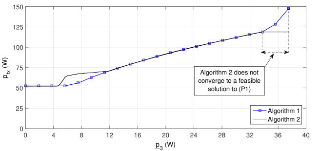
Figure 6: Performance comparison between centralized control (Algorithm 1) versus distributed control (Algorithm 2).

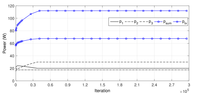
Figure 7: Convergence performance of Algorithm $2$.

V Power Region Characterization

In this section, we characterize the achievable power region for the receiver loads without versus with time sharing. First, we propose a time-sharing scheme to schedule multiuser power transfer by connecting/disconnecting loads to/from their receivers over time. We then propose a centralized algorithm to jointly optimize the time allocation and load resistance of receivers for time sharing based power transmission, by extending that for (P1) in Section IV for the case without time sharing. Last, numerical examples are provided to compare the power-region performance of the multiuser MRC-WPT system without versus with time sharing.

V-A Multiuser Power Transfer with Time Sharing

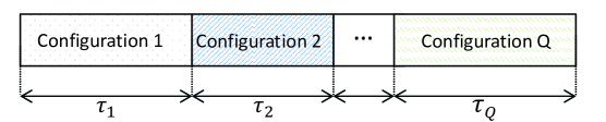
Figure 8: Time-sharing based multiuser power transfer.

As shown in Fig. 8, there are in general $Q=2^{N}-1$ time-sharing configurations for transferring power to $N$ receiver loads depending on the state of each receiver’s switch. We index these configurations by $q$, $q\in{\cal Q}=\{1,\ldots,Q\}$. Specifically, let ${\cal S}=\{(s_{1},\ldots,s_{N})~{}|~{}s_{n}\in\{0,1\},~{}\forall n\in{\cal N}\}$ denote the set consisting of all possible states of receiver switches. Without loss of generality, we remove the trivial case that all switches are open, i.e., $s_{n}=0$, $\forall n\in\cal N$, from $\cal S$ by setting ${\cal S}\leftarrow{\cal S}\setminus\{(0,...,0)\}$. As a result, we have the cardinality of $\cal S$ as $|{\cal S}|=Q$. For convenience, we assign an one-to-one mapping between the elements in the two sets $\cal{Q}$ and $\cal S$, i.e., we assign each configuration $q\in\cal Q$ to one switch state $(s_{1},\ldots,s_{N})\in\cal S$. By default, we assign configuration $q=1$ to $(s_{1},\ldots,s_{N})=(1,\ldots,1)$, i.e., all switches are closed.

Let $\tau>0$ denote the total time available for power transmission. Let the time allocated for the power transmission under configuration $q$ be denoted by $\tau_{q}$, with $0\leq\tau_{q}\leq\tau$. We thus have $\sum_{q\in\cal Q}\tau_{q}\leq\tau$, where the strict inequality occurs when the required energy, $\overline{p}_{n}\tau$, $n=1,...,N$, at all loads are satisfied by the end of $Q$-slot transmissions, where the voltage source at the transmitter can be switched off for the remaining time ($\tau-\sum_{q\in{\cal Q}}\tau_{q})>0$ to save energy. Over all configurations, the average transmitter power and the average power delivered to each load $n$ can be obtained from (8) and (9), respectively, as follows:

$$p_{\text{tx}}=\sum_{q\in{\cal Q}}\dfrac{|v_{\text{tx}}|^{2}}{2\tau}\dfrac{1}{r_{\text{tx}}+w^{2}\sum_{k\in{\cal N}_{q}}h_{k}^{2}\left(r_{k}+x_{k,q}\right)^{-1}}\tau_{q},$$ (21)

$$p_{n}=\sum_{q\in{\cal Q}_{n}}\dfrac{|v_{\text{tx}}|^{2}}{2\tau}\dfrac{w^{2}h_{n}^{2}x_{n,q}\left(r_{n}+x_{n,q}\right)^{-2}}{\left(r_{\text{tx}}+w^{2}\sum_{k\in{\cal N}_{q}}h_{k}^{2}\left(r_{k}+x_{k,q}\right)^{-1}\right)^{2}}\tau_{q},$$ (22)

where $x_{n,q}$ is the resistance value of load $n$ under configuration $q$. Furthermore, ${\cal N}_{q}\subseteq\cal N$ denotes the subset of receivers with their loads connected under configuration $q$, while ${\cal Q}_{n}\subseteq\cal Q$ denotes the subset of configurations under which receiver $n$ has its load connected. Compared to the previous case without time sharing, the time allocation $\tau_{q}$’s, $\forall q\in\cal Q$, can provide extra degrees of freedom for performance optimization.

V-B Power Region Definition

The power region is defined as the set of power-tuples achievable for all loads with a given transmission time $\tau$ subject to their adjustable resistance values. Specifically, the power region for the case without time sharing (i.e., all loads receive power concurrently) is defined as

$${\cal R}_{\text{without-TS}}=\bigcup_{\{\underline{x}_{n}\leq x_{n}\leq\overline{x}_{n}\}_{n\in\cal N}}(p_{1},\ldots,p_{N}),$$ (23)

with $p_{n}$’s, $\forall n\in\cal N$, are given in (9). Similarly, the power region for the case with time sharing is defined as

$${\cal R}_{\text{with-TS}}=\bigcup_{\begin{subarray}{c}\{0\leq\tau_{q}\leq\tau,\}_{q\in\cal Q},~{}\sum_{q\in\cal Q}\tau_{q}\leq\tau\\ \{\underline{x}_{n}\leq x_{n,q}\leq\overline{x}_{n}\}_{n\in{\cal N},q\in\cal Q}\end{subarray}}(p_{1},\ldots,p_{N}),$$ (24)

with $p_{n}$’s, $\forall n\in\cal N$, are given in (22). It is evident that the power region with time sharing is no smaller than that without time sharing in general, i.e., ${\cal R}_{\text{without-TS}}\subseteq{\cal R}_{\text{with-TS}}$, since by simply setting $\tau_{1}=\tau$ and $\tau_{q}=0$, $\forall q\neq 1$, we have ${\cal R}_{\text{without-TS}}={\cal R}_{\text{with-TS}}$.

V-C Centralized Algorithm with Time Sharing: Revised

In this subsection, we extend the centralized algorithm in Section III without time sharing to the case with time sharing by jointly optimizing the time allocation and load resistance of all receivers to minimize the transmitter power subject to the given load (average received power) constraints. Hence, we consider problem (P4) as follows.

$$\mathrm{(P4)}:\mathop{\mathtt{min}}_{\begin{subarray}{c}\{0\leq\tau_{q}\leq\tau\}_{q\in\cal Q},~{}\{\underline{x}_{n}\leq x_{n,q}\leq\overline{x}_{n}\}_{n\in{\cal N},q\in{\cal Q}}\end{subarray}} ~{}\sum_{q\in{\cal Q}}\dfrac{|v_{\text{tx}}|^{2}}{2\tau}\dfrac{1}{\hskip 5.69054ptr_{\text{tx}}+w^{2}\sum_{k\in{\cal N}_{q}}h_{k}^{2}\left(r_{k}+x_{k,q}\right)^{-1}\hskip 5.69054pt}\tau_{q}$$ (25)

$$\mathtt{s.t.} ~{}\sum_{q\in{\cal Q}_{n}}\dfrac{|v_{\text{tx}}|^{2}}{2\tau}\dfrac{w^{2}h_{n}^{2}x_{n,q}(r_{n}+x_{n,q})^{-2}}{\left(r_{\text{tx}}+w^{2}\sum_{k\in{\cal N}_{q}}h_{k}^{2}\left(r_{k}+x_{k,q}\right)^{-1}\right)^{2}}\tau_{q}\geq\underline{p}_{n},~{}\forall n\in\cal N,$$ (26)

$$~{}\sum_{q\in\cal Q}\tau_{q}\leq\tau.$$ (27)

Although (P4) is non-convex, we can apply the technique of alternating optimization to solve it sub-optimally in general, as discussed below. Since (P1) is assumed feasible, the feasibility of (P4) is ensured due to the fact that ${\cal R}_{\text{without-TS}}\subseteq{\cal R}_{\text{with-TS}}$.

Initialize $\tau_{1}=\tau$ and $x_{n,1}=x_{n}^{*}$, $\forall n\in\cal N$, where $(x_{1}^{*},\ldots,x_{N}^{*})$ denotes the optimal solution to (P1) for the case without time sharing. Moreover, initialize $\tau_{q}=0$ and $x_{n,q}=\min\{\hskip 1.99168pt\max\{\big{(}{r_{n}r_{\textnormal{tx}}+w^{2}h_{n}^{2}}\big{)}/r_{\textnormal{tx}},\hskip 1.99168pt\underline{x}_{n}\},\hskip 1.99168pt\overline{x}_{n}\}$, $\forall n\in\cal N$, $\forall q\neq 1$. At each iteration $itr$, $itr=1,2,\ldots$, we design $\tau_{q}$’s and $x_{n,q}$’s alternatively according to the following procedure. First, we solve (P4) over $\tau_{q}$’s, $\forall q\in\cal Q$, while the rest of variables are all fixed. The resulting problem is a linear programming (LP) which can be efficiently solved using the existing software, e.g. CVX [26]. We update $\tau_{q}$’s as the obtained solution. Next, we optimize the load resistance for different configurations sequentially, e.g., starting from configuration $1$ to $Q$. For each configuration $q$, we solve (P4) over $x_{n,q}$’s, $\forall n\in\cal N$, with the rest of variables all being fixed. We thus consider the optimization problem (P4$-$q) as follows.

$$\mathrm{(P4-q)}:\mathop{\mathtt{min}}_{\{\underline{x}_{n}\leq x_{n,q}\leq\overline{x}_{n}\}_{n\in{\cal N}}} ~{}\dfrac{|v_{\text{tx}}|^{2}}{2\tau}\dfrac{1}{\hskip 5.69054ptr_{\text{tx}}+w^{2}\sum_{k\in{\cal N}_{q}}h_{k}^{2}(r_{k}+x_{k,q})^{-1}\hskip 5.69054pt}\tau_{q}$$ (28)

$$\mathtt{s.t.} ~{}\dfrac{|v_{\text{tx}}|^{2}}{2\tau}\dfrac{w^{2}h_{n}^{2}x_{n,q}\left(r_{n}+x_{n,q}\right)^{-2}}{\left(r_{\text{tx}}+w^{2}\sum_{k\in{\cal N}_{q}}h_{k}^{2}(r_{k}+x_{k,q})^{-1}\right)^{2}}\tau_{q}\geq\underline{p}_{n}-p_{n,-q},~{}\forall n\in\cal N.$$ (29)

where $p_{n,-q}=\sum_{m\in{\cal Q}_{n}\setminus\{q\}}|v_{\text{tx}}|^{2}w^{2}h_{n}^{2}x_{n,m}(r_{n}+x_{n,m})^{-2}\tau_{m}/(2\tau(r_{\text{tx}}+w^{2}\sum_{k\in{\cal N}_{m}}h_{k}^{2}(r_{k}+x_{k,m})^{-1})^{2})$. For each receiver $n$, its load power constraint given in (26) is re-expressed in (29), where all power terms that do not involve $x_{n,q}$, $\forall n\in\cal N$, are moved to the right-hand side (RHS) of the inequality, denoted by $p_{n,-q}$, which is treated as constant in (P4$-$q). From (22), it follows that $p_{n,-q}$ denotes the average power delivered to load $n$ under all other configurations, $m\in{\cal Q}_{n}\setminus\{q\}$. Problem (P4$-$q) has the same structure as (P1); as a result, we can solve it using an algorithm similar to Algorithm $1$. We then update $x_{n,q}$’s, $\forall n\in\cal N$, as the obtained solution to (P4$-$q). At the end of each iteration $itr$, we compute $p_{\text{tx}}^{(itr)}$ as the objective value given in (25). The algorithm stops when $\Delta p_{\text{tx}}=p_{\text{tx}}^{(itr-1)}-p_{\text{tx}}^{(itr)}\leq\Delta p$ holds, with $p_{\text{tx}}^{(0)}=\infty$ by default and $\Delta p>0$ denoting a given stopping threshold. The above alternating optimization based algorithm for (P4) is summarized in Table V, denoted as Algorithm $3$.

TABLE V: Algorithm for (P4).

  Algorithm $3$  

• Initialize $itr=1$, $\Delta p>0$ and $\Delta p_{\text{tx}}=p_{\text{tx}}^{(0)}=\infty$. Initialize $\tau_{1}=\tau$ and $x_{n,1}=x_{n}^{*}$, $\forall n\in\cal N$. Initialize $\tau_{q}=0$ and $x_{n,q}=\min\{\hskip 1.99168pt\max\{\big{(}{r_{n}r_{\textnormal{tx}}+w^{2}h_{n}^{2}}\big{)}/r_{\textnormal{tx}},\hskip 1.99168pt\underline{x}_{n}\},\hskip 1.99168pt\overline{x}_{n}\}$, $\forall n\in\cal N$, $\forall q\neq 1$.

• While $\Delta p_{\text{tx}}>\Delta p$ do:

  • Solve (P4) over $\tau_{q}$’s, $\forall q\in\cal Q$, assuming that the rest of variables are all fixed. Update $\tau_{q}$’s as the optimal solution to the resulting problem.

  • For $q=1$ to $q=Q$ do :

    • Solve (P4$-$q) using similar algorithm as Algorithm $1$. Update $x_{n,q}$’s, $\forall n\in\cal N$, as the solution to (P4$-$q).

  • Compute (25) and save the obtained value as $p_{\text{tx}}^{(itr)}$. Accordingly, set $\Delta p_{\text{tx}}=p_{\text{tx}}^{(itr-1)}-p_{\text{tx}}^{(itr)}$.

  • Set $itr=itr+1$.

• Return $x_{n,q}$’s and $\tau_{q}$’s as the solution to (P4).

 

Note that the convergence of Algorithm 3 for (P4) is ensured since the objective value of (P4), i.e., $p_{\text{tx}}^{(itr)}$, is non-increasing over iterations, while the constraints in (26) and (27) are all satisfied at each iteration.

V-D Numerical Example

We consider the same system setup as that in Section III-B. We set $\underline{x}_{n}=1\Omega$ and $\overline{x}_{n}=100\Omega$, $\forall n\in\cal N$. For Algorithm $3$ in the case with time sharing, we set $\Delta p=10^{-3}$.

Figs. 9(a), 9(b), and 9(c) show power regions ${\cal R}_{\text{without-TS}}$ versus ${\cal R}_{\text{with-TS}}$ given by (23) and (24), respectively, under three different resonant angular frequencies of $w=14.2\times 10^{6}$rad/sec, $w=42.6\times 10^{6}$rad/sec, and $w=127.8\times 10^{6}$rad/sec, respectively. For the purpose of exposition, we consider only the two-user case for Fig. 9 by assuming receiver $3$ is disconnected from its load, i.e., $s_{3}=0$ (see Fig. 2). It is observed that ${\cal R}_{\text{with-TS}}$ is always larger than ${\cal R}_{\text{without-TS}}$, as expected. It is also observed that the power region difference becomes less significant as the operating frequency decreases. This result is explained as follows. When $w$ is sufficiently small, the power delivered to each load $n$ in the case without time sharing, given in (9), can be approximated as $p_{n}\approx|v_{\text{tx}}|^{2}w^{2}h_{n}^{2}x_{n}(r_{n}+x_{n})^{-2}/(2r_{\text{tx}}^{2})$, from which it follows that there is no evident coupling effect among receivers. In this regime, given load resistance $x_{n}$, the power received by load $n$ does not depend on whether the other receivers are connected to their loads or not. Thus, time sharing is less effective and hence cannot enlarge the power region over that without time sharing. Last, note that since Algorithm $3$ for (P4) in general obtains a suboptimal solution, ${\cal R}_{\text{with-TS}}$ shown in Fig. 9 is only an achievable power region under the time-sharing scenario.

Next, we consider again the case with all three users in Fig. 2. We also fix $w=42.6\times 10^{6}$rad/sec and $\underline{p}_{1}=\underline{p}_{2}=5$W. Fig. 10 compares the transmitter power $p_{\text{tx}}$ obtained using Algorithms $1$ and $3$ over $\underline{p}_{3}$, with $0<\underline{p}_{3}\leq 55.9$W, where Algorithm $3$ takes at most $4$ iterations to converge. It is observed that Algorithm $3$ achieves lower $p_{\text{tx}}$ than Algorithm $1$ over all values of $\underline{p}_{3}$. This result is expected due to the fact that time sharing provides extra degrees of freedom for multiuser power transmission scheduling. Consequently, the time allocation and load resistance for the receivers can be jointly optimized to further reduce the transmitter power as compared to the case without time sharing when only load resistance is optimized.

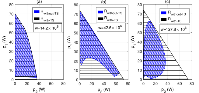
Figure 9: Power regions without versus with time sharing.

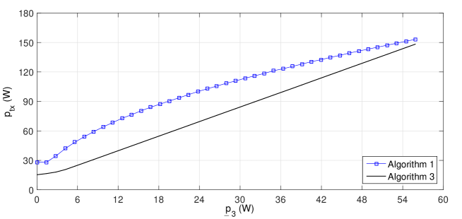
Figure 10: Performance comparison between Algorithm $1$ (without time sharing) versus Algorithm $3$ (with time sharing).

VI Conclusion

In this paper, we have studied a point-to-multipoint WPT system via MRC. We derive closed-form expressions for the input and output power in terms of the system parameters for arbitrary number of receivers. Similar to other multiuser wireless applications such as those in wireless communication and far-field microwave based WPT, a near-far fairness issue is revealed in our considered MRC-WPT system. To tackle this problem, we propose a centralized charging control algorithm for jointly optimizing the receivers’ load resistance to minimize the transmitter power subject to the given load power constraints. For ease of practical implementation, we also propose a distributed algorithm for receivers to iteratively adjust their load resistance based on local information and one-bit feedback from each of the other receivers. We show by simulation that the distributed algorithm performs very close to the centralized algorithm with a finite number of iterations. Last, we characterize the achievable multiuser power regions for the loads without and with time sharing and compare them through numerical examples. It is shown that time sharing can help further mitigate the near-far issue by enlarging the achievable power region as compared to the case without time sharing. As a concluding remark, we would like to point out that MRC-WPT is a promising new research area in which many tools from signal processing and optimization can be applied to devise innovative solutions, and we hope that this paper will open up an avenue for more future works along this direction.

-A Proof of Proposition III.1

From (8), it follows that

$$\dfrac{\partial p_{\text{tx}}}{\partial x_{n}}=\dfrac{|v_{\text{tx}}|^{2}}{2}\dfrac{w^{2}h_{n}^{2}(r_{n}+x_{n})^{-2}}{\left(r_{\text{tx}}+w^{2}\sum_{k=1}^{N}h_{k}^{2}\left(r_{k}+x_{k}\right)^{-1}\right)^{2}},$$ (30)

where it can be easily verified that $\partial p_{\text{tx}}/\partial x_{n}>0$ over $x_{n}>0$. This means that $p_{\text{tx}}$ strictly increases over $x_{n}>0$. The proof of Proposition III.1 is thus completed.

-B Proof of Proposition III.2

From (9), it follows that for $m\neq n$,

$$\dfrac{\partial p_{m}}{\partial x_{n}}=\dfrac{|v_{\text{tx}}|^{2}}{2}\dfrac{2w^{4}x_{m}h_{m}^{2}h_{n}^{2}\left(r_{m}+x_{m}\right)^{-2}\left(r_{n}+x_{n}\right)^{-2}}{\left(r_{\text{tx}}+w^{2}\sum_{k=1}^{N}h_{k}^{2}(r_{k}+x_{k})^{-1}\right)^{3}},$$ (31)

where it can be easily verified that $\partial p_{m}/\partial x_{n}>0$ over $x_{n}>0$. This means that $p_{m}$, $m\neq n$, strictly increases over $x_{n}>0$. Similarly, for $m=n$, from (9), it follows that

$$\dfrac{\partial p_{n}}{\partial x_{n}}=\dfrac{|v_{\text{tx}}|^{2}}{2}\dfrac{w^{2}h_{n}^{2}\left(r_{n}+x_{n}\right)^{-3}}{\left(r_{\text{tx}}+w^{2}\sum_{k=1}^{N}h_{k}^{2}(r_{k}+x_{k})^{-1}\right)^{3}}\bigg{(}w^{2}h_{n}^{2}$$

$$\hskip 108.12047pt+\left(r_{\text{tx}}+\phi_{n}\right)\left(r_{n}-x_{n}\right)\bigg{)},$$ (32)

where $\phi_{n}=w^{2}\sum_{k\in{\cal N}\setminus\{n\}}h_{k}^{2}(r_{k}+x_{k})^{-1}$. It can be easily verified that $\partial p_{n}/\partial x_{n}>0$ over $0<x_{n}<\dot{x}_{n}$, with $\dot{x}_{n}>0$ given in (12), and $\partial p_{n}/\partial x_{n}<0$ over $x_{n}>\dot{x}_{n}$. The proof of Proposition III.2 is thus completed.

-C Proof of Proposition III.3

Since $\partial p_{\text{sum}}/\partial x_{n}=\sum_{k=1}^{N}\partial p_{k}/\partial x_{n}$, we can easily prove Proposition III.3 using the same argument for the proof of Proposition III.2. The detail is thus omitted for brevity.

-D Proof of Proposition III.4

From (10), it follows that

$$\dfrac{\partial\rho}{\partial x_{n}}=\dfrac{|v_{\text{tx}}|^{2}}{2}\dfrac{w^{2}h_{n}^{2}\left(r_{n}+x_{n}\right)^{-4}}{\left(r_{\text{tx}}+w^{2}\sum_{k=1}^{N}h_{k}^{2}(r_{k}+x_{k})^{-1}\right)^{2}}\bigg{(}2r_{n}\varphi_{n}x_{n}$$

$$+r_{n}w^{2}h_{n}^{2}+x_{n}^{2}\left(\varphi_{n}-\phi_{n}-r_{\text{tx}}\right)+r_{n}^{2}\left(\varphi_{n}+\phi_{n}+r_{\text{tx}}\right)\bigg{)}.$$ (33)

Accordingly, it can be verified that when $\varphi_{n}-\phi_{n}-r_{\text{tx}}\geq 0$, $\rho$ strictly increases over $x_{n}>0$. Otherwise, if $\varphi_{n}-\phi_{n}-r_{\text{tx}}<0$, then $\rho$ increases over $0<x_{n}<\dddot{x}_{n}$ due to the fact that $x_{n}^{2}(\varphi_{n}-\phi_{n}-r_{\text{tx}})+2r_{n}\varphi_{n}x_{n}+r_{n}w^{2}h_{n}^{2}+r_{n}^{2}(\varphi_{n}+\phi_{n}+r_{\text{tx}})<0$ and the rest of terms in the right-hand side of (-D) are all positive; similarly $\rho$ declines over $x_{n}>\dddot{x}$. The proof of Proposition III.4 is thus completed.

-E Impedance Characterization of EM Coils

As shown in Fig. 11, we consider two circular EM coils, indexed by $i$, $i\in\{1,2\}$, in the free space (no external electric and/or magnetic fields exist). Without loss of generality, we assume that the center of EM coil $1$ is located at the origin, i.e., $(x=0,y=0,z=0)$, and its surface normal vector is given by $\vec{n}_{1}=\vec{z}$. On the other hand, we assume that the center of EM coil $2$ is located at $(x=x^{\prime},y=y^{\prime},z=z^{\prime})$ and its surface normal vector is given by $\vec{n}_{2}=n_{x,2}\vec{x}+n_{y,2}\vec{y}+n_{z,2}\vec{z}$, with $\sqrt{n_{x,2}^{2}+n_{y,2}^{2}+n_{z,2}^{2}}=1$. As shown in Fig. 12, we assume that each EM coil $i$ consists of $b_{i}$ closely wound turns of round shaped wire, where the inner radius of coil is denoted by $e_{\text{inner},i}>0$, while the outer radius is denoted by $e_{\text{outer},i}>e_{\text{inner},i}$.

Figure 11: A system of two circular EM coils.

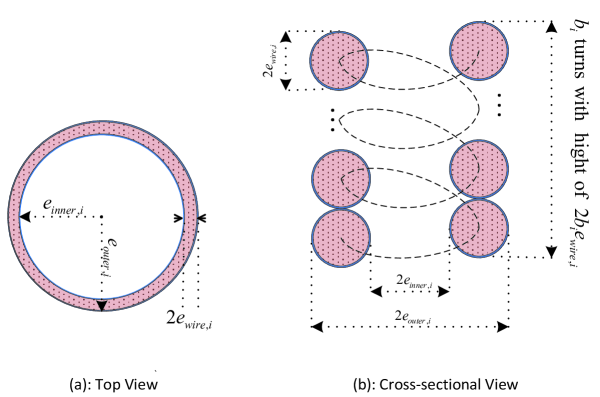
Figure 12: Circular EM coil.

Accordingly, the average radius of each EM coil $i$ and the radius of the wire used to build this coil are obtained as $e_{\text{ave},i}=(e_{\text{outer},i}+e_{\text{inner},i})/2$ and $e_{\text{wire},i}=(e_{\text{outer},i}-e_{\text{inner},i})/2$, respectively. Let $r_{i}$ and $l_{i}$ denote the resistance and self-inductance of each EM coil $i$. Given $e_{\text{wire},i}\ll e_{\text{ave},i}$, i.e., the wire is much thinner than the average radius, which is practically valid, we thus have [7]:

$$r_{i} =\dfrac{2\sigma_{i}b_{i}e_{\text{ave},i}}{e_{\text{wire},i}^{2}},$$ (34)

$$l_{i} =b_{i}^{2}e_{\text{ave},i}\mu\big{(}\ln(\dfrac{8e_{\text{ave},i}}{e_{\text{wire},i}})-2\big{)},$$ (35)

where $\sigma_{i}$ is the resistivity of the wire used in EM coil $i$ and $\mu=4\pi\times 10^{-7}$N/A², which denotes the magnetic permeability of the air. Let $h$ denote the mutual inductance between the two EM coils. By assuming $d\triangleq\sqrt{{x^{\prime}}^{2}+{y^{\prime}}^{2}+{z^{\prime}}^{2}}\gg e_{\text{ave},1},e_{\text{ave},2}$, i.e., the distance between the two EM coils is much larger than their average radiuses, we have [23]:

$$h=-\dfrac{\pi\mu b_{1}b_{2}e_{\text{ave},1}^{2}e_{\text{ave},2}^{2}}{4d^{3}} \bigg{(}3\cos(\theta^{\prime})\sin(\theta^{\prime})\cos(\phi^{\prime})n_{x,2}$$

$$+3\cos(\theta^{\prime})\sin(\theta^{\prime})\sin(\phi^{\prime})n_{y,2}$$

$$+(2\cos^{2}(\theta^{\prime})-\sin^{2}(\theta^{\prime}))n_{z,2}\bigg{)},$$ (36)

where $\theta^{\prime}=\cos^{-1}(z^{\prime}/d)$ and $\phi^{\prime}=\tan^{-1}(y^{\prime}/x^{\prime})$.

References

- [1] M. R. V. Moghadam and R. Zhang, “Multiuser charging control in wireless power transfer via magnetic resonant coupling,” IEEE Int. Conf. Acoustics, Speech and Signal Processing (ICASSP), pp. 3182-3186, Apr. 2015.
- [2] J. Murakami, F. Sato, T. Watanabe, H. Matsuki, S. Kikuchi, K. Harakawa, and T. Satoh, “Consideration on cordless power station-contactless power transmission system,” IEEE Trans. Magn., vol. 32, no. 5, pp. 5037-5039, Sep. 1996.
- [3] C. Kim, D. Seo, J. You, J. Park, and B. H. Cho, “Design of a contactless battery charger for cellular phone,” IEEE Trans. Ind. Electron., vol. 48, no. 6, pp. 1238-1247, Dec. 2001.
- [4] A. Kurs, A. Karalis, R. Moffatt, J. D. Joannopoulos, P. Fisher, and M. Soljacic, “Wireless power transfer via strongly coupled magnetic resonances,” Science, vol. 317, no. 83, pp. 83-86, July 2007.
- [5] Z. Fei, S. A. Hackworth, F. Weinong, L. Chengliu, M. Zhihong, and S. Mingui, “Relay effect of wireless power transfer using strongly coupled magnetic resonances,” IEEE Trans. Magn., vol. 47, no. 5, pp. 1478-1481, May 2011.
- [6] J. Shin, S. Shin, Y. Kim, S. Ahn, S. Lee, G. Jung, S. Jeon, and D. Cho, “Design and implementation of shaped magnetic-resonance-based wireless power transfer system for roadway-powered moving electric vehicles,” IEEE Trans. Ind. Electron., vol. 61, no. 3, pp. 1179-1192, Mar. 2014.
- [7] L. Chen, Y. C. Zhou, and T. J. Cui, “An optimizable circuit structure for high-efficiency wireless power transfer,” IEEE Trans. Ind. Electron., vol. 60, no. 1, pp. 339-349, Jan. 2013.
- [8] B. L. Cannon, J. F. Hoburg, D. D. Stancil, and S. C. Goldstein, “Magnetic resonant coupling as a potential means for wireless power transfer to multiple small receivers,” IEEE Trans. Power Electron., vol. 24, no. 7, pp. 1819-1825, July 2009.
- [9] O. Jonah, S. V. Georgkopoulos, and M. M. Tentzeris, “Optimal design parameters for wireless power transfer by resonance magnetic,” IEEE Antennas Wireless Propagat. Lett., vol. 11, pp. 1390-1393, Nov. 2012.
- [10] Y. Zhang and Z. Zhao, “Frequency splitting analysis of two-coil resonant wireless power transfer,” IEEE Antennas Wireless Propagat. Lett., vol. 13, pp. 400-402, Feb. 2014.
- [11] Y. Zhang, Z. Zhao, and K. Chen, “Frequency decrease analysis of resonant wireless power transfer,” IEEE Trans. Power Electron., vol. 29, no. 13, pp. 1058-1063, Mar. 2014.
- [12] I. Yoon and H. Ling, “Investigation of near-field wireless power transfer under multiple transmitters,” IEEE Antennas Wireless Propagat. Lett., vol. 10, pp. 662-665, June 2011.
- [13] K. Lee and D. Cho, “Diversity analysis of multiple transmitters in wireless power transfer system,” IEEE Trans. Magn., vol. 49, no. 6, pp. 2946-2952, June 2013.
- [14] D. Ahn and S. Hong, “Effect of coupling between multiple transmitters or multiple receivers on wireless power transfer,” IEEE Trans. Ind. Electron., vol. 60, no. 7, pp. 2602-2613, July 2013.
- [15] J. Garnica, R. A. Chinga, and J. Lin, “Wireless power transmission: from far field to near field,” Proceedings of the IEEE, vol. 101, no. 6, pp. 1321-1331, June 2013.
- [16] R. Johari, J. V. Krogmeier, and D. J. Love, “Analysis and practical considerations in implementing multiple transmitters for wireless power transfer via coupled magnetic resonance,” IEEE Trans. Ind. Electron., vol. 61, no. 4, pp. 1174-1783, Apr. 2014.
- [17] J. Jadidian and D. Katabi. “Magnetic MIMO: how to charge your phone in your pocket,” Proceedings of the 20th annual international conference on Mobile computing and networking (ACM), pp. 495-506, Sep. 2014.
- [18] B. H. Waters, B. J. Mahoney, V. Ranganathan, and J. R. Smith, “Power delivery and leakage field control using an adaptive phased-array wireless power system,” IEEE Trans. Power Electron., vol. 30, no. 11, pp. 6298-6309, Nov. 2015.
- [19] H. Lang, A. Ludwig, and C. D. Sarris, “Convex optimization of wireless power transfer systems with multiple transmitters,” IEEE Trans. Antennas Propag., vol. 62, no. 9, pp. 4623-4636, Sept. 2014.
- [20] R. Zhang and C. K. Ho, “MIMO broadcasting for simultaneous wireless information and power transfer,” IEEE Trans. Wireless Commun., vol. 12, no. 5, pp. 1989-2001, May 2013.
- [21] J. Xu and R. Zhang, “Energy beamforming with one-bit feedback,” IEEE Trans. Sig. Process., vol. 62, no. 20, pp. 5370-5381, Oct. 2014.
- [22] R. Tseng, B. Novak, S. Shevde, and K. Grajski, “Introduction to the alliance for wireless power loosely-coupled wireless power transfer system specification version 1.0,” in Proceedings of IEEE Wireless Power Transfer (WPT), May 2013.
- [23] D. Cheng, Field and wave electromagnetics, Addison Wesley, 1983.
- [24] Z. Pantic and M. Lukic, “Framework and topology for active tuning of parallel compensated receivers in power transfer systems,” IEEE Trans. Power Electron., vol. 27, no. 11, pp. 4503-4513, Nov. 2012.
- [25] S. Boyd and L. Vandenberghe, Convex optimization, Cambridge University Press, 2004.
- [26] M. Grant and S. Boyd, “CVX: Matlab software for disciplined convex programming”, version 2.0 beta, available online at http://cvxr.com/cvx, Sept. 2013.