High-order accurate physical-constraints-preserving finite difference WENO schemes for special relativistic hydrodynamics

Abstract

The paper develops high-order accurate physical-constraints-preserving finite difference WENO schemes for special relativistic hydrodynamical (RHD) equations, built on the local Lax-Friedrich splitting, the WENO reconstruction, the physical-constraints-preserving flux limiter, and the high-order strong stability preserving time discretization. They are extensions of the positivity-preserving finite difference WENO schemes for the non-relativistic Euler equations [21]. However, developing physical-constraints-preserving methods for the RHD system becomes much more difficult than the non-relativistic case because of the strongly coupling between the RHD equations, no explicit formulas of the primitive variables and the flux vectors with respect to the conservative vector, and one more physical constraint for the fluid velocity in addition to the positivity of the rest-mass density and the pressure. The key is to prove the convexity and other properties of the admissible state set and discover a concave function with respect to the conservative vector instead of the pressure which is an important ingredient to enforce the positivity-preserving property for the non-relativistic case.

Several one- and two-dimensional numerical examples are used to demonstrate accuracy, robustness, and effectiveness of the proposed physical-constraints-preserving schemes in solving RHD problems with large Lorentz factor, or strong discontinuities, or low rest-mass density or pressure etc.

1 Introduction

The paper is concerned with developing high-order accurate numerical methods for special relativistic hydrodynamical (RHD) equations. In the laboratory frame, the $(d+1)$-dimensional space-time RHD equations may be written into a system of conservation laws as follows

$$\frac{\partial\mbox{\boldmath\small$U$}}{\partial t}+\sum^{d}_{i=1}\frac{\partial\mbox{\boldmath\small$F$}_{i}(\mbox{\boldmath\small$U$})}{\partial x_{i}}=0,$$ (1.1)

where $U$ and $\mbox{\boldmath\small$F$}_{i}$ are the conservative vector and the flux in the $x_{i}$-direction, respectively, defined by

$$\mbox{\boldmath\small$U$}= \big{(}D,m_{1},\cdots,m_{d},E\big{)}^{T},$$

$$\mbox{\boldmath\small$F$}_{i}= \big{(}Dv_{i},m_{1}v_{i}+p\delta_{1,i},\cdots,m_{d}v_{i}+p\delta_{d,i},m_{i}\big{)}^{T},~{}~{}i=1,\cdots,d,$$

with the mass density $D=\rho W$, the momentum density vector $\mbox{\boldmath\small$m$}=DhW\mbox{\boldmath\small$v$}$, and the energy density $E=DhW-p$, respectively. Here $\rho$, $p$, and $\mbox{\boldmath\small$v$}=(v_{1},\cdots,v_{d})^{T}$ denote the rest-mass density, the kinetic pressure, and the fluid velocity respectively, $W=1/\sqrt{1-v^{2}}$ is the Lorentz factor with $v=(v_{1}^{2}+\cdots+v_{d}^{2})^{1/2}$, and $h$ denotes the specific enthalpy defined by

$$h=1+e+\displaystyle{\frac{p}{\rho}},$$ (1.2)

with units in which the speed of light is equal to one, and $e$ is the specific internal energy.

The system (1.1) has taken into account the relativistic description of fluid dynamics where the fluid flow is at nearly speed of light in vacuum and appears in investigating numerous astrophysical phenomena from stellar to galactic scales, e.g. formation of black holes, coalescing neutron stars, core collapse super-novae, X-ray binaries, active galactic nuclei, super-luminal jets and gamma-ray bursts, etc. However, it still involves highly nonlinear equations due to the Lorentz factor so that its analytic treatment is extremely difficult. A powerful and primary approach to improve our understanding of the physical mechanisms in RHDs is through numerical simulations. Comparing to the non-relativistic case, the numerical difficulties are coming from strongly nonlinear coupling between the RHD equations, which leads to no explicit expression of the primitive variables $\mbox{\boldmath\small$V$}=(\rho,\mbox{\boldmath\small$v$},p)^{T}$ and the flux vector $\mbox{\boldmath\small$F$}_{i}$ in terms of $U$, and some physical constraints such as $\rho>0$, $p>0$, $E\geq D$, and $1>v$ etc. Its numerical study did not attract considerable attention until 1990s.

The first attempt to numerically solve the RHD equations was made by using a finite difference method with the artificial viscosity technique in Lagrangian or Eulerian coordinates, see [31, 32, 48, 49]. After that, various modern shock-capturing methods were gradually developed for the special RHDs since 1990s, e.g. the HLL (Harten-Lax-van Leer-Einfeldt) method [43], the two-shock approximation solvers [1, 8], the flux corrected transport method [11], the Roe solver [13], the HLLC (Harten-Lax-van Leer-Contact) approximate Riemann solver [37], the flux-splitting method based on the spectral decomposition [10], Steger-Warming flux vector splitting method [69], and the kinetic schemes [57, 27, 39]. Besides those, high-order accurate schemes for the RHD system were also studied, e.g. ENO (essentially non-oscillatory) and weighted ENO methods [9, 60, 46], the piecewise parabolic methods [33, 38], the space-time conservation element and solution element method [40], and the discontinuous Galerkin (DG) method [42], the Runge-Kutta DG methods with WENO (weighted ENO) limiter [70], the direct Eulerian GRP schemes [58, 59, 51], the adaptive moving mesh methods [18, 19, 20], and genuinely multi-dimensional finite volume local evolution Galerkin method [50]. The readers are also referred to the early review articles [23, 34, 14].

The above existing works do not preserve the positivity of the rest-mass density and the pressure and the bounds of the fluid velocity. Although they have been used to simulate some RHD flows successfully, there exists the big risk of failure when they are applied to RHD problems with large Lorentz factor, or low density or pressure, or strong discontinuity, because the negative density or pressure, or the larger velocity than the speed of light may be obtained so that the calculated eigenvalues of the Jacobian matrix become imaginary, in other words, the discrete problem becomes ill-posed. In practice, the nonphysical numerical solutions are usually simply replaced with a “close” and “physical” one by performing recalculation with more diffusive schemes and smaller CFL number until the numerical solutions become physical, see e.g. [61, 22]. Obviously, such approch is not scientifically reasonable to a certain extent, and it is of great significance to develop high-order accurate numerical schemes, whose solutions satisfy the intrinsic physical constraints. Recently, there exist some works on the maximum-principle-satisfying schemes for scalar hyperbolic conservation law [62, 67], the positivity-preserving schemes for the non-relativistic Euler equations with or without source terms [66, 63, 64], the positivity-preserving well-balanced schemes for the shallow water equations [53], the positivity preserving semi-Lagrangian DG method for the Vlasov-Poisson system [41], and Lagrangian method with positivity-preserving limiter for multi-material compressible flow [5]. A class of the parametrized maximum principle preserving and positivity-preserving flux limiters were also well-developed via decoupling some linear or nonlinear constraints for the high order accurate schemes for scalar hyperbolic conservation laws [56, 29], nonlinear convection-dominated diffusion equations [25], compressible Euler equations [54] and ideal magnetohydrodynamical equations [6] as well as simulating incompressible flows [55]. A survey of the maximum-principle-satisfying or positivity-preserving high-order schemes is presented in [65].

The aim of the paper is to do the first attempt in the aspect of developing the high-order accurate physical-constraints-preserving finite difference schemes for special RHD equations (1.1). Such attempt is nontrivial in comparison of the non-relativistic case, because of the strongly nonlinear coupling between the RHD equations due to the Lorentz factor, no explicit formulas of $V$ and $\mbox{\boldmath\small$F$}_{i}$ with respect to $U$, and one more physical constraint for the fluid velocity in addition to the positivity of the rest-mass density and the pressure. The key will be to prove the convexity and other properties of the admissible state set and discover a concave function with respect to the conservative vector $U$ instead of the pressure, which is an important ingredient to enforce the positivity-preserving property for the non-relativistic case. The paper is organized as follows. Section 2 discusses the admissible state set and its properties of the special RHD equations. They play a pivotal role in studying the physical-constraints-preserving property of numerical schemes. Section 3 presents the high-order accurate physical-constraints-preserving finite difference WENO schemes for the RHD equations. Section 3.1 considers detailedly one-dimensional case with spatial discretization in Section 3.1.1 and time discretization in Section 3.1.2. Section 3.2 gives the 2D extension of the above scheme and apply it to the 2D axisymmetric case. Section 4 gives several 1D and 2D numerical experiments to demonstrate accuracy, robustness and effectiveness of the proposed schemes for relativistic problems with large Lorentz factor, or strong discontinuities, or low rest-mass density or pressure etc. Section 5 concludes the paper with several remarks.

2 Properties of RHD equations

This section discusses the admissible state set and its properties for the RHD equations (1.1). Throughout the paper, the equation of state (EOS) will be restricted to the $\Gamma$–law

$$p=(\Gamma-1)\rho e,$$ (2.1)

with the adiabatic index $\Gamma\in(1,2]$. Such restriction on $\Gamma$ is reasonable under the compressibility assumptions, see [7].

The RHD system (1.1) with (2.1) is identical to the $d$-dimensional non-relativistic Euler equations in the formal structure, and also satisfies the rotational invariance and the homogeneity as well as the hyperbolicity in time, see [69]. The momentum equations in (1.1) are only with a Lorentz-contracted momentum density replacing $\rho v_{i}$ in the non-relativistic Euler equations. When the fluid velocity is much smaller than the speed of light (i.e. $v\ll 1$) and the velocity of the internal (microscopic) motion of the fluid particles is small, the system (1.1) reduces to the non-relativistic Euler equations. The $(d+2)$ real eigenvalues of the Jacobian matrix $\mbox{\boldmath\small$A$}_{i}(\mbox{\boldmath\small$U$})={\partial\mbox{\boldmath\small$F$}_{i}(\mbox{\boldmath\small$U$})}/{\partial\mbox{\boldmath\small$U$}}$ for (1.1) with (2.1) are

$$\lambda_{i}^{(1)} =\frac{{v_{i}(1-c_{s}^{2})-c_{s}W^{-1}\sqrt{1-v_{i}^{2}-(v^{2}-v_{i}^{2})c_{s}^{2}}}}{{1-v^{2}c_{s}^{2}}},$$

$$\lambda_{i}^{(2)} =\cdots=\lambda_{i}^{(d+1)}=v_{i},$$

$$\lambda_{i}^{(d+2)} =\frac{{v_{i}(1-c_{s}^{2})+c_{s}W^{-1}\sqrt{1-v_{i}^{2}-(v^{2}-v_{i}^{2})c_{s}^{2}}}}{{1-v^{2}c_{s}^{2}}},$$

for $i=1,\cdots,d$, where the local sound speed $c_{s}=\sqrt{\frac{\Gamma p}{\rho h}}$. However, relations between the laboratory quantities ($D$, $m_{i}$, and $E$) and the quantities in the local rest frame ($\rho$, $v_{i}$, and $e$) introduce a strong coupling between the hydrodynamic equations and pose more additional numerical difficulties than the non-relativistic case. For example, the flux vectors $\mbox{\boldmath\small$F$}_{i}$ and the primitive variable vector $\mbox{\boldmath\small$V$}:=(\rho,\mbox{\boldmath\small$v$},p)^{T}$ can not be formulated in explicit forms of the conservative vector $U$, and some constraints (e.g. $\rho>0$, $p>0$, and $1>v$, etc.) should be fulfilled by the physical solution $U$.

Definition 2.1

The set of (physically) admissible states of the RHD equations (1.1) with (2.1) is defined by

$${\mathcal{G}}=\left\{{\left.\mbox{\boldmath\small$U$}=(D,\mbox{\boldmath\small$m$},E)^{T}\right|{\rho(\mbox{\boldmath\small$U$})>0,~{}p(\mbox{\boldmath\small$U$})>0,~{}1>v(\mbox{\boldmath\small$U$})}}\right\}.$$ (2.2)

Such definition is very natural and intuitive but unpractical when giving the value of the conservative vector $U$, because there is no explicit expression of the primitive variable $\mbox{\boldmath\small$V$}=(\rho,\mbox{\boldmath\small$v$},p)^{T}$ in terms to $U$ for the system (1.1). It is this feature that makes the discussions on the admissible state and the physical-constraints-preserving schemes presented later nontrivial or even challenging for RHD equations (1.1). In practical computations, for given $\mbox{\boldmath\small$U$}=(D,\mbox{\boldmath\small$m$},E)^{T}$, one has to (iteratively) solve a nonlinear algebraic equation such as

$$E+p=DW+\displaystyle\frac{\Gamma}{\Gamma-1}pW^{2},$$ (2.3)

by any standard root-finding algorithm to get the pressure $p(\mbox{\boldmath\small$U$})$. Then $v_{i}$ and $\rho$ are sequentially calculated by

$$v_{i}(\mbox{\boldmath\small$U$})=\frac{m_{i}}{{E+p(\mbox{\boldmath\small$U$})}},\quad\rho(\mbox{\boldmath\small$U$})=D\sqrt{1-v^{2}(\mbox{\boldmath\small$U$})}.$$ (2.4)

Note that the Lorentz factor $W$ in (2.3) has been rewritten into $\left(1-m^{2}/(E+p)^{2}\right)^{-1/2}$ with $m:=(m_{1}^{2}+\cdots+m_{d}^{2})^{1/2}$. Existence of the unique positive solution to the pressure equation (2.3) is given in the proof of Lemma 2.1. It is worth mentioning that different from the non-relativistic case, such positive solution $p(\mbox{\boldmath\small$U$})$ is not a concave function of $U$ generally, see Fig. 2.1.

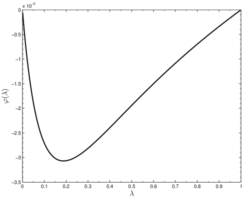
Figure 2.1: The function $\varphi(\lambda):=p(\lambda\mbox{\boldmath\small$U$}^{(1)}+(1-\lambda)\mbox{\boldmath\small$U$}^{(0)})-\lambda p(\mbox{\boldmath\small$U$}^{(1)})-(1-\lambda)p(\mbox{\boldmath\small$U$}^{(0)})$ with $\mbox{\boldmath\small$U$}^{(0)}=(2,1.2,8)^{\rm T}\in{\mathcal{G}}$ and $\mbox{\boldmath\small$U$}^{(1)}=(2,5,35)^{\rm T}\in{\mathcal{G}}$. The value of $\varphi(\lambda)$ is always less than zero when $\lambda\in(0,1)$.

A practical and equivalent definition of ${\mathcal{G}}$ is given as follows.

Lemma 2.1

The admissible set ${\mathcal{G}}$ defined in (2.2) is equivalent to the following set

$${\mathcal{G}}_{1}=\left\{{\mbox{\boldmath\small$U$}=(D,\mbox{\boldmath\small$m$},E)^{T}\left|{D>0,~{}q(\mbox{\boldmath\small$U$}):=E-\sqrt{D^{2}+m^{2}}>0}\right.}\right\}.$$ (2.5)

• (i): Prove that $\mbox{\boldmath\small$U$}\in{\mathcal{G}}_{1}$ when $\mbox{\boldmath\small$U$}\in{\mathcal{G}}$. When $\mbox{\boldmath\small$U$}=(D,\mbox{\boldmath\small$m$},E)^{T}$ satisfy the constraints $\rho(\mbox{\boldmath\small$U$})>0$, $p(\mbox{\boldmath\small$U$})>0$, and $v(\mbox{\boldmath\small$U$})<1$, it is not difficult to show

  $$D=\frac{\rho}{{\sqrt{1-v^{2}(\mbox{\boldmath\small$U$})}}}>0,\quad E=\frac{{\rho h}}{{1-v^{2}(\mbox{\boldmath\small$U$})}}-p>\rho h-p\overset{\eqref{eq:h}}{=}\rho(1+e)>0,$$

  and

  $$E^{2}- \left({D^{2}+m^{2}}\right)=\left({\frac{{\rho h}}{{1-v^{2}}}-p}\right)^{2}-\frac{{\rho^{2}}}{{1-v^{2}}}-\left({\frac{{\rho hv}}{{1-v^{2}}}}\right)^{2}$$

  $$=\left({\frac{{\rho h}}{{1-v^{2}}}}\right)^{2}+p^{2}-2p{\frac{{\rho h}}{{1-v^{2}}}}-\frac{{\rho^{2}}}{{1-v^{2}}}-\left({\frac{{\rho hv}}{{1-v^{2}}}}\right)^{2}$$

  $$=\frac{1}{{1-v^{2}}}\left[{\left({\rho h-p}\right)^{2}-\rho^{2}-p^{2}v^{2}}\right]\overset{\eqref{eq:h}}{=}\frac{1}{{1-v^{2}}}\left[{\rho^{2}\left({1+e}\right)^{2}-\rho^{2}-p^{2}v^{2}}\right]$$

  $$\overset{v<1}{>}\frac{1}{{1-v^{2}}}\left[{\rho^{2}\left({1+e}\right)^{2}-\rho^{2}-p^{2}}\right]\overset{\eqref{gamma-law}}{=}\frac{{\rho^{2}e}}{{1-v^{2}}}\big{(}2+e\Gamma(2-\Gamma)\big{)}\overset{\Gamma\in(1,2]}{>}0.$$

  Thus $q(\mbox{\boldmath\small$U$})=E-\sqrt{D^{2}+m^{2}}>0$ so that $\mbox{\boldmath\small$U$}\in{\mathcal{G}}_{1}$.

  (ii): Prove that $\mbox{\boldmath\small$U$}\in{\mathcal{G}}$ when $\mbox{\boldmath\small$U$}\in{\mathcal{G}}_{1}$. Consider the function of $p$ defined by

  $$\Phi(p):=\frac{{m^{2}}}{{E+p}}+D\sqrt{1-\frac{{m^{2}}}{{(E+p)^{2}}}}+\frac{p}{{\Gamma-1}}-E,\quad p\in[0,+\infty),$$

  with $U$ satisfying that $D>0$ and $E>\sqrt{D^{2}+m^{2}}$. Obviously, $\Phi(p)\in C^{1}[0,+\infty)$, and

  $$\Phi^{\prime}(p)=\frac{1}{{\Gamma-1}}-\frac{{m^{2}}}{{\left({E+p}\right)^{2}}}\left({1-\frac{D}{{\sqrt{(E+p)^{2}-m^{2}}}}}\right)\geq 1-\frac{{m^{2}}}{{\left({E+p}\right)^{2}}}>0,\quad\forall p\in\left[{0,+\infty}\right),$$

  when $E>\sqrt{D^{2}+m^{2}}$ and $\Gamma\in(1,2]$. Thus $\Phi(p)$ is a strictly monotonically increasing function of $p$ in the interval $[0,+\infty)$. On the other hand, one has

  $$\Phi(0)=\frac{{m^{2}}}{E}+D\sqrt{1-\frac{{m^{2}}}{{E^{2}}}}-E=\left({D-\sqrt{E^{2}-m^{2}}}\right)\sqrt{1-\frac{{m^{2}}}{{E^{2}}}}<0,$$

  and $\mathop{\lim}\limits_{p\to+\infty}\Phi(p)=+\infty$ because

  $$\mathop{\lim}\limits_{p\to+\infty}\frac{{\Phi(p)}}{p}=\frac{1}{{\Gamma-1}}>0.$$

  Thanks to the intermediate value theorem and the monotonicity of $\Phi(p)$, there exists a unique positive solution to the equation $\Phi(p)=0$, which is equivalent to the equation (2.3). Denote this positive solution by $p(\mbox{\boldmath\small$U$})$. Substituting this into (2.4) may give

  $${v(\mbox{\boldmath\small$U$})}=\frac{{m}}{{E+p(\mbox{\boldmath\small$U$})}}<\frac{{m}}{E}<1,\quad\rho(\mbox{\boldmath\small$U$})=D\sqrt{1-{v^{2}(\mbox{\boldmath\small$U$})}}>0,$$

  by using the conditions that $D>0$ and $E>\sqrt{D^{2}+m^{2}}$. Thus $\mbox{\boldmath\small$U$}\in{\mathcal{G}}$ and the proof is completed.       

Remark 2.1

Comparing to ${\mathcal{G}}$ defined in (2.2), the constraints on conservative variables in the set ${\mathcal{G}}_{1}$ is much easier to be verified when the value of $U$ is given.

With the help of equivalence of the admissible state set ${\mathcal{G}}$ in Lemma 2.1, we can further prove that it is a convex set.

Lemma 2.2

The admissible set ${\mathcal{G}}_{1}$ is a convex set.

• To show that the set ${\mathcal{G}}_{1}$ is convex, one has to prove that for all $\lambda$ in the interval $[0,1]$, and all $\mbox{\boldmath\small$U$}^{(0)}=(D^{(0)},\mbox{\boldmath\small$m$}^{(0)},E^{(0)})^{T}$ and $\mbox{\boldmath\small$U$}^{(1)}=(D^{(1)},\mbox{\boldmath\small$m$}^{(1)},E^{(1)})^{T}$ in the set ${\mathcal{G}}_{1}$, the point $\lambda\mbox{\boldmath\small$U$}^{(1)}+(1-\lambda)\mbox{\boldmath\small$U$}^{(0)}=:(D^{(\lambda)},\mbox{\boldmath\small$m$}^{(\lambda)},E^{(\lambda)})^{T}\in{\mathcal{G}}_{1}$ also belongs to ${\mathcal{G}}_{1}$.

  Because $\mbox{\boldmath\small$U$}^{(0)},\mbox{\boldmath\small$U$}^{(1)}\in{\mathcal{G}}_{1}$, one has

  $$D^{(\lambda)}=\lambda D^{(1)}+(1-\lambda)D^{(0)}>0,$$

  and

  $$E^{(\lambda)} =\lambda E^{(1)}+(1-\lambda)E^{(0)}$$

  $$>\lambda\sqrt{\left({D^{(1)}}\right)^{2}+\sum\limits_{i=1}^{d}\left(m_{i}^{(1)}\right)^{2}}+(1-\lambda)\sqrt{\left({D^{(0)}}\right)^{2}+\sum\limits_{i=1}^{d}{\left({m_{i}^{(0)}}\right)^{2}}}$$

  $$\geq\sqrt{\left[{\lambda D^{(1)}+(1-\lambda)D^{(0)}}\right]^{2}+\sum\limits_{i=1}^{d}{\left[{\lambda\left|{m_{i}^{(1)}}\right|+(1-\lambda)\left|{m_{i}^{(0)}}\right|}\right]^{2}}}$$

  $$\geq\sqrt{\left({D^{(\lambda)}}\right)^{2}+\sum\limits_{i=1}^{d}{\left({m_{i}^{(\lambda)}}\right)^{2}}}.$$

  Here the Minkowski inequality for both vectors $(\lambda D^{(1)},\lambda m_{1}^{(1)},\cdots,\lambda m_{d}^{(1)})$ and $((1-\lambda)D^{(0)},(1-\lambda)m_{1}^{(0)},\cdots,(1-\lambda)m_{d}^{(0)})$ and the triangle inequality $|\lambda m_{i}^{(1)}+(1-\lambda)m_{i}^{(0)}|\leq\lambda|m_{i}^{(1)}|+(1-\lambda)|m_{i}^{(0)}|$ have been used respectively. Thus $\lambda\mbox{\boldmath\small$U$}^{(1)}+(1-\lambda)\mbox{\boldmath\small$U$}^{(0)}\in{\mathcal{G}}_{1}$ for all $\lambda\in[0,1]$. The proof is completed.       

Remark 2.2

The proof of Lemma 2.2 implies that the function $q(\mbox{\boldmath\small$U$})$ defined in (2.5) is concave. Moreover, the function $q(\mbox{\boldmath\small$U$})$ is also Lipschitz continuous with respect to $U$ and satisfies

$$\left|{q(\mbox{\boldmath\small$U$}^{(1)})-q(\mbox{\boldmath\small$U$}^{(0)})}\right| \leq\left|{E^{(1)}-E^{(0)}}\right|+\left|{\sqrt{\left({D^{(1)}}\right)^{2}+\left(m^{(1)}\right)^{2}}-\sqrt{\left({D^{(0)}}\right)^{2}+\left(m^{(0)}\right)^{2}}}\right|$$

$$\leq\left|{E^{(1)}-E^{(0)}}\right|+{\sqrt{\left({D^{(1)}-D^{(0)}}\right)^{2}+\sum_{i=1}^{d}\left({m^{(1)}_{i}-m^{(0)}_{i}}\right)^{2}}}$$

$$\leq\sqrt{2\left[{\left({D^{(1)}-D^{(0)}}\right)^{2}+\sum_{i=1}^{d}\left({m^{(1)}_{i}-m^{(0)}_{i}}\right)^{2}+\left({E^{(1)}-E^{(0)}}\right)^{2}}\right]}$$

$$=\sqrt{2}\left\|{\mbox{\boldmath\small$U$}^{(1)}-\mbox{\boldmath\small$U$}^{(0)}}\right\|,$$ (2.6)

for any $\mbox{\boldmath\small$U$}^{(0)}=(D^{(0)},\mbox{\boldmath\small$m$}^{(0)},E^{(0)})^{T}\in\mathbb{R}^{d+2}$ and $\mbox{\boldmath\small$U$}^{(1)}=(D^{(1)},\mbox{\boldmath\small$m$}^{(1)},E^{(1)})^{T}\in\mathbb{R}^{d+2}$, where the inequality $a+b\leq\sqrt{2(a^{2}+b^{2})}$ has been used. The concavity and Lipschitz continuity of $q(\mbox{\boldmath\small$U$})$ will play a pivotal role in designing our physical-constraints-preserving schemes for the RHD equations (1.1).

By means of the convexity of ${\mathcal{G}}$, the following properties of ${\mathcal{G}}$ can further be verified.

Lemma 2.3

Assume $\mbox{\boldmath\small$U$}\in{\mathcal{G}}_{1}$, then

1. $\lambda\mbox{\boldmath\small$U$}\in{\mathcal{G}}_{1}$, for all $\lambda>0$.

2. $\mbox{\boldmath\small$T$}\mbox{\boldmath\small$U$}\in{\mathcal{G}}_{1}$, where $\mbox{\boldmath\small$T$}=\mbox{diag}\{1,\mbox{\boldmath\small$T$}_{d\times d},1\}$ and $\mbox{\boldmath\small$T$}_{d\times d}$ is the $d\times d$ rotational matrix.

3. $\mbox{\boldmath\small$U$}\pm{\alpha}^{-1}{{\mbox{\boldmath\small$F$}_{i}(\mbox{\boldmath\small$U$})}}\in{\mathcal{G}}_{1}$ for all real number $\alpha\geq\varrho_{i}$, $i=1,\cdots,d$, where $\varrho_{i}$ is the spectral radius of the Jacobian matrix $\mbox{\boldmath\small$A$}_{i}(\mbox{\boldmath\small$U$})$, i.e.

   $$\varrho_{i}:=\frac{{\left|{v_{i}}\right|(1-c_{s}^{2})+c_{s}W^{-1}\sqrt{1-v_{i}^{2}-(v^{2}-v_{i}^{2})c_{s}^{2}}}}{{1-v^{2}c_{s}^{2}}}.$$

• The verification of first two properties are omitted here because they can be directly and easily verified via the definition of ${\mathcal{G}}_{1}$.

The following will prove the third conclusion (iii) that if $\mbox{\boldmath\small$U$}\in{\mathcal{G}}_{1}$, then $\left({D^{\pm},\mbox{\boldmath\small$m$}^{\pm},E^{\pm}}\right)^{T}=\mbox{\boldmath\small$U$}^{\pm}:=\mbox{\boldmath\small$U$}\pm{\alpha}^{-1}{{\mbox{\boldmath\small$F$}_{1}(\mbox{\boldmath\small$U$})}}\in{\mathcal{G}}_{1}$. It is nontrivial and requires several techniques thanks to no explicit formulas of the flux $\mbox{\boldmath\small$F$}_{1}(\mbox{\boldmath\small$U$})$ in terms of $U$.

For all $\mbox{\boldmath\small$U$}\in{\mathcal{G}}_{1}$ and the perfact gas (2.1) with $\Gamma\in(1,2]$, one has

$$c_{s}^{2}=\frac{{\Gamma p}}{{\rho h}} =\frac{{\Gamma p}}{{\rho+\frac{\Gamma}{{\Gamma-1}}p}}<\Gamma-1\leq 1,$$ (2.7)

so that the inequalities

$$W^{-1}\sqrt{1-v_{i}^{2}-(v^{2}-v_{i}^{2})c_{s}^{2}}\geq W^{-1}\sqrt{1-v^{2}}=1-v^{2},$$

and

$$\varrho_{1}\geq\frac{{|v_{1}|}(1-c_{s}^{2})+c_{s}(1-v^{2})}{1-v^{2}c_{s}^{2}},$$

hold. They imply

$$1-\frac{{\left|{v_{1}}\right|}}{\varrho_{1}} \geq 1-\frac{\left|v_{1}\right|(1-v^{2}c_{s}^{2})}{{|v_{1}|}(1-c_{s}^{2})+c_{s}(1-v^{2})}=\frac{{W^{-2}c_{s}\left({1-\left|{v_{1}}\right|c_{s}}\right)}}{{\left|{v_{1}}\right|\left({1-c_{s}^{2}}\right)+c_{s}(1-v^{2})}}$$

$$\geq\frac{{W^{-2}c_{s}\left({1-\left|{v_{1}}\right|c_{s}}\right)}}{{\left|{v_{1}}\right|\left({1-c_{s}^{2}}\right)+c_{s}(1-v_{1}^{2})}}=\frac{{W^{-2}c_{s}}}{{\left|{v_{1}}\right|+c_{s}}}>\frac{{W^{-2}c_{s}}}{{1+c_{s}}},$$

so that one has

$${1\pm\frac{{v_{1}}}{\alpha}}\geq{1-\frac{{\left|{v_{1}}\right|}}{\alpha}}\geq{1-\frac{{\left|{v_{1}}\right|}}{{\varrho_{1}}}}>\frac{{W^{-2}c_{s}}}{{1+c_{s}}}>0.$$ (2.8)

Thus one gets

$$D^{\pm} =D\left({1\pm\frac{{v_{1}}}{\alpha}}\right)>0,$$

$$E^{\pm} =E\pm\frac{{m_{1}}}{\alpha}=(\rho hW^{2}-p)\pm\rho hW^{2}\frac{{v_{1}}}{\alpha}\overset{\eqref{EQ-thz01}}{>}\frac{{\rho hc_{s}}}{{1+c_{s}}}-p\overset{\eqref{EQ-thz02}}{=}p\left({\frac{\Gamma}{{c_{s}(1+c_{s})}}-1}\right)$$

$$\overset{\eqref{EQ-thz02}}{>}p\left({\frac{\Gamma}{{\Gamma-1+\sqrt{\Gamma-1}}}-1}\right)=p\left({\frac{{1-\sqrt{\Gamma-1}}}{{\Gamma-1+\sqrt{\Gamma-1}}}}\right)\overset{\Gamma\in(1,2]}{\geq}0,$$

and

$$\left({D^{\pm}}\right)^{2}+(\mbox{\boldmath\small$m$}^{\pm})^{2}-\left({E^{\pm}}\right)^{2}$$

$$=\left({1\pm\frac{{v_{1}}}{\alpha}}\right)^{2}\left({D^{2}+m^{2}-E^{2}}\right)\pm\frac{{2p}}{\alpha}\left({m_{1}-Ev_{1}}\right)\left({1\pm\frac{{v_{1}}}{\alpha}}\right)+\frac{{p^{2}}}{{\alpha^{2}}}(1-v_{1}^{2})$$

$$=\left({1\pm\frac{{v_{1}}}{\alpha}}\right)^{2}W^{2}\left[{\rho^{2}+p^{2}v^{2}-\left({\rho h-p}\right)^{2}}\right]+p^{2}\left({1\pm\frac{{v_{1}}}{\alpha}}\right)^{2}-p^{2}+\frac{{p^{2}}}{{\alpha^{2}}}$$

$$=\left({1\pm\frac{{v_{1}}}{\alpha}}\right)^{2}W^{2}\left[{\rho^{2}+p^{2}-\left({\rho+\frac{p}{{\Gamma-1}}}\right)^{2}}\right]+p^{2}\left({\frac{1}{{\alpha^{2}}}-1}\right)$$

$$\leq\left({1-\frac{{\left|{v_{1}}\right|}}{{\varrho_{1}}}}\right)^{2}W^{2}\left[{\rho^{2}+p^{2}-\left({\rho+\frac{p}{{\Gamma-1}}}\right)^{2}}\right]+p^{2}\left({\frac{1}{{\varrho_{1}^{2}}}-1}\right),$$ (2.9)

here (2.8) and $\rho^{2}+p^{2}-\left({\rho+\frac{p}{{\Gamma-1}}}\right)^{2}\leq 0$ have been used. Note that $\varrho_{1}$ is a positive solution to the following quadratic equation

$$(1-v^{2}c_{s}^{2})\varrho_{1}^{2}-2\left|{v_{1}}\right|(1-c_{s}^{2})\varrho_{1}+{v_{1}^{2}(1-c_{s}^{2})-c_{s}^{2}(1-v^{2})}=0,$$

which is equivalent to

$$\left({1-\varrho_{1}^{2}}\right)c_{s}^{2}=W^{2}\left({\varrho_{1}-\left|{v_{1}}\right|}\right)^{2}(1-c_{s}^{2}).$$ (2.10)

It implies that $\varrho_{1}<1$. With the help of (2.9) and (2.10), one has

$$\left({D^{\pm}}\right)^{2}+(\mbox{\boldmath\small$m$}^{\pm})^{2}-\left({E^{\pm}}\right)^{2}$$

$$\leq\left({\frac{1}{{\varrho_{1}^{2}}}-1}\right)\frac{{c_{s}^{2}}}{{1-c_{s}^{2}}}\left[{p^{2}-\frac{{2\rho p}}{{\Gamma-1}}-\frac{{p^{2}}}{{\left({\Gamma-1}\right)^{2}}}}\right]+p^{2}\left({\frac{1}{{\varrho_{1}^{2}}}-1}\right)$$

$$=\left({\frac{1}{{\varrho_{1}^{2}}}-1}\right)\frac{{p^{2}}}{{(1-c_{s}^{2})\left({\Gamma-1}\right)}}\left[{\Gamma-1-c_{s}^{2}\left({\frac{1}{{\Gamma-1}}+\frac{{2\rho}}{p}}\right)}\right]$$

$$\overset{\Gamma\in(1,2]}{\leq}\left({\frac{1}{{\varrho_{1}^{2}}}-1}\right)\frac{{p^{2}}}{{(1-c_{s}^{2})\left({\Gamma-1}\right)}}\left[{1-c_{s}^{2}\left({\frac{1}{{\Gamma-1}}+\frac{{2\rho}}{p}}\right)}\right]$$

$$=\left({\frac{1}{{\varrho_{1}^{2}}}-1}\right)\frac{{p^{2}}}{{(1-c_{s}^{2})\left({\Gamma-1}\right)}}\cdot\frac{1-2\Gamma}{h}\overset{\Gamma\in(1,2]}{<}0.$$

Thus $\mbox{\boldmath\small$U$}\pm{\alpha}^{-1}{{\mbox{\boldmath\small$F$}_{1}(\mbox{\boldmath\small$U$})}}\in{\mathcal{G}}_{1}$. Combining the above deduction and the property (ii) may verify $\mbox{\boldmath\small$U$}\pm{\alpha}^{-1}{{\mbox{\boldmath\small$F$}_{i}(\mbox{\boldmath\small$U$})}}\in{\mathcal{G}}_{1}$ for $i=2,\cdots,d$. For example, in the case of $d=3$, $T$ may be taken as

$$\mbox{\boldmath\small$T$}_{\theta,\phi}:=\left[{\begin{array}[]{*{20}c}1&0&0&0&0\\ 0&{\cos\theta\sin\phi}&{\sin\theta\sin\phi}&{\cos\phi}&0\\ 0&{-\sin\theta}&{\cos\theta}&0&0\\ 0&{-\cos\theta\cos\phi}&{-\sin\theta\cos\phi}&{\sin\phi}&0\\ 0&0&0&0&1\end{array}}\right],$$

for all $\theta\in[0,2\pi),\phi\in[0,\pi]$. Using the property (ii) that $\mbox{\boldmath\small$T$}_{\theta,\phi}\mbox{\boldmath\small$U$}\in{\mathcal{G}}_{1}$ and the above proof of the property (iii) gives

$$\mbox{\boldmath\small$T$}_{\theta,\phi}\mbox{\boldmath\small$U$}\pm{\alpha}^{-1}{{\mbox{\boldmath\small$F$}_{1}(\mbox{\boldmath\small$T$}_{\theta,\phi}\mbox{\boldmath\small$U$})}}\in{\mathcal{G}}_{1},$$

where $\alpha$ is not less than $\varrho_{1}$. Since $\mbox{\boldmath\small$T$}_{\theta,\phi}^{-1}$ is also a rotational matrix, it holds that

$$\mbox{\boldmath\small$T$}_{\theta,\phi}^{-1}\left({\mbox{\boldmath\small$T$}_{\theta,\phi}\mbox{\boldmath\small$U$}\pm{\alpha}^{-1}{{\mbox{\boldmath\small$F$}_{1}(\mbox{\boldmath\small$T$}_{\theta,\phi}\mbox{\boldmath\small$U$})}}}\right)=\mbox{\boldmath\small$U$}\pm{\alpha}^{-1}{{\mbox{\boldmath\small$T$}_{\theta,\phi}^{-1}\mbox{\boldmath\small$F$}_{1}(\mbox{\boldmath\small$T$}_{\theta,\phi}\mbox{\boldmath\small$U$})}}\in{\mathcal{G}}_{1}.$$

With the help of the rotational invariance of the system (1.1), see [69], one has $\mbox{\boldmath\small$U$}\pm{\alpha}^{-1}{{\mbox{\boldmath\small$F$}_{i}(\mbox{\boldmath\small$U$})}}\in{\mathcal{G}}_{1}$ for $\forall\alpha\geq\varrho_{i},~{}i=2,3$. The proof is completed.       

It is worth emphasizing that Lemma 2.3 also plays a pivotal role in seeking the physical-constraints-preserving schemes.

3 Numerical schemes

This section gives the physical-constraints-preserving finite difference WENO schemes for the RHD system (1.1) with the EOS (2.1).

3.1 One-dimensional case

This subsection first discusses numerical discretization of the 1D RHD equations in the laboratory frame

$$\frac{\partial\mbox{\boldmath\small$U$}}{\partial t}+\frac{\partial\mbox{\boldmath\small$F$}_{1}(\mbox{\boldmath\small$U$})}{\partial x}=0,$$ (3.1)

where

$$\mbox{\boldmath\small$U$}=(D,m_{1},E)^{T},\ \ \mbox{\boldmath\small$F$}_{1}=(Dv_{1},m_{1}v_{1}+p,m_{1})^{T}.$$

3.1.1 Spatial discretization

Let us divide the space into cells of size $\Delta x$, and denote the $j$th cell by $I_{j}=\left(x_{j-\frac{1}{2}},x_{j+\frac{1}{2}}\right)$, where $x_{j+\frac{1}{2}}=\frac{1}{2}(x_{j}+x_{j+1})$ and $x_{j}=j\Delta x$, $j\in\mathbb{Z}$.

A semi-discrete, $(2r-1)$th-order accurate, conservative finite difference scheme of the 1D RHD equations (3.1) may be written as

$$\frac{{d\mbox{\boldmath\small$U$}_{j}(t)}}{{dt}}=-\frac{1}{{\Delta x}}\left({\widehat{\mbox{\boldmath\small$F$}}_{j+\frac{1}{2}}-\widehat{\mbox{\boldmath\small$F$}}_{j-\frac{1}{2}}}\right)=:{\cal L}(\mbox{\boldmath\small$U$}(t);j),$$ (3.2)

where $\mbox{\boldmath\small$U$}_{j}(t)\approx\mbox{\boldmath\small$U$}(x_{j},t)$ and the numerical flux $\widehat{\mbox{\boldmath\small$F$}}_{j+\frac{1}{2}}$ is consistent with the flux vector $\mbox{\boldmath\small$F$}_{1}(\mbox{\boldmath\small$U$})$ and satisfies

$$\frac{1}{{\Delta x}}\Big{(}{\widehat{\mbox{\boldmath\small$F$}}_{j+\frac{1}{2}}-\widehat{\mbox{\boldmath\small$F$}}_{j-\frac{1}{2}}}\Big{)}=\partial_{x}\mbox{\boldmath\small$F$}_{1}(\mbox{\boldmath\small$U$})|_{x_{j}}+{\cal O}(\Delta x^{2r-1}).$$

Definition 3.1

The scheme (3.2) is physical-constraints-preserving if $\mbox{\boldmath\small$U$}_{j}(t)+\Delta t{\cal L}\left({\mbox{\boldmath\small$U$}(t)};j\right)\in{\mathcal{G}}$ for all $j\in\mathbb{Z}$, under a CFL-type condition for $\Delta t$ when $\mbox{\boldmath\small$U$}_{j}(t)\in{\mathcal{G}}$ for all $j$.

The third property of Lemma 2.3 has implied that there at least exists a physical-constraints-preserving scheme for the 1D RHD system (3.1). An example is the first-order (i.e. $r=1$) accurate local Lax-Friedrichs scheme with the numerical flux

$$\widehat{\mbox{\boldmath\small$F$}}_{j+\frac{1}{2}}=\widehat{\mbox{\boldmath\small$F$}}_{j+\frac{1}{2}}^{\rm LLF}:=\frac{1}{2}\big{(}{\mbox{\boldmath\small$F$}_{1}(\mbox{\boldmath\small$U$}_{j})+\mbox{\boldmath\small$F$}_{1}(\mbox{\boldmath\small$U$}_{j+1})-\alpha_{j+\frac{1}{2}}\left({\mbox{\boldmath\small$U$}_{j+1}-\mbox{\boldmath\small$U$}_{j}}\right)}\big{)},$$

where the viscosity coefficient $\alpha_{j+\frac{1}{2}}:=\max\left\{{\varrho_{1}\left({\mbox{\boldmath\small$U$}_{j-r+1}}\right),\cdots,\varrho_{1}\left({\mbox{\boldmath\small$U$}_{j+r}}\right)}\right\}$. In practical computations, the above $\alpha_{j+\frac{1}{2}}$ may be replaced with

$$\alpha_{j+\frac{1}{2}}=\vartheta\max\left\{{\varrho_{j+\frac{1}{2}}^{ROE},\varrho_{1}\left({\mbox{\boldmath\small$U$}_{j-r+1}}\right),\cdots,\varrho_{1}\left({\mbox{\boldmath\small$U$}_{j+r}}\right)}\right\}.$$

see [2], where the parameter $\vartheta$ is typically in the range of 1.1 to 1.3 and controls the amount of dissipation in the numerical schemes while $\varrho_{j+\frac{1}{2}}^{ROE}$ is the spectral radius of the Roe matrix $\widehat{\mbox{\boldmath\small$A$}}_{1}(\mbox{\boldmath\small$U$}_{j},\mbox{\boldmath\small$U$}_{j+1})$ approximating the Jacobian matrix $\mbox{\boldmath\small$A$}_{1}(\mbox{\boldmath\small$U$})$, see [13].

The physical-constraints-preserving property of the above local Lax-Friedrichs scheme is shown below.

Lemma 3.1

If $\mbox{\boldmath\small$U$}_{j}\in{\mathcal{G}}$ for all $j$, then under the CFL-type condition

$$\Delta t\leq\frac{{\Delta x}}{{2\mathop{\max}\limits_{j}\alpha_{j+\frac{1}{2}}}},$$ (3.3)

one has

$$\mbox{\boldmath\small$U$}_{j}^{\pm,\rm LLF}:=\mbox{\boldmath\small$U$}_{j}\mp\frac{{2\Delta t}}{{\Delta x}}\widehat{\mbox{\boldmath\small$F$}}_{j\pm\frac{1}{2}}^{\rm LLF}\in{\mathcal{G}},$$

and $\mbox{\boldmath\small$U$}_{j}(t)+\Delta t{\cal L}\left({\mbox{\boldmath\small$U$}(t)};j\right)=\frac{1}{2}\left(\mbox{\boldmath\small$U$}_{j}^{+,\rm LLF}+\mbox{\boldmath\small$U$}_{j}^{-,\rm LLF}\right)\in{\mathcal{G}}$ for all $j$.

• Note that $\mbox{\boldmath\small$U$}_{j}^{\pm,\rm LLF}$ can be rewritten as

  $$\mbox{\boldmath\small$U$}_{j}^{\pm,\rm LLF} =\mbox{\boldmath\small$U$}_{j}\mp\frac{{\Delta t}}{{\Delta x}}\big{(}{\mbox{\boldmath\small$F$}_{1}(\mbox{\boldmath\small$U$}_{j})+\mbox{\boldmath\small$F$}_{1}(\mbox{\boldmath\small$U$}_{j\pm 1})\mp\alpha_{j\pm\frac{1}{2}}\left({\mbox{\boldmath\small$U$}_{j\pm 1}-\mbox{\boldmath\small$U$}_{j}}\right)}\big{)}$$

  $$=\left({1-2\alpha_{j\pm\frac{1}{2}}\frac{{\Delta t}}{{\Delta x}}}\right)\mbox{\boldmath\small$U$}_{j}+\alpha_{j\pm\frac{1}{2}}\frac{{\Delta t}}{{\Delta x}}\left[\left({\mbox{\boldmath\small$U$}_{j}\mp\frac{{\mbox{\boldmath\small$F$}_{1}(\mbox{\boldmath\small$U$}_{j})}}{{\alpha_{j\pm\frac{1}{2}}}}}\right)+\left({\mbox{\boldmath\small$U$}_{j\pm 1}\mp\frac{{\mbox{\boldmath\small$F$}_{1}(\mbox{\boldmath\small$U$}_{j\pm 1})}}{{\alpha_{j\pm\frac{1}{2}}}}}\right)\right],$$

  which is a convex combination under the CFL-type condition (3.3). Utilizing the property (iii) of Lemma 2.3 implying that

  $$\mbox{\boldmath\small$U$}_{j}\mp\frac{{\mbox{\boldmath\small$F$}_{1}(\mbox{\boldmath\small$U$}_{j})}}{{\alpha_{j\pm\frac{1}{2}}}},~{}\mbox{\boldmath\small$U$}_{j\pm 1}\mp\frac{{\mbox{\boldmath\small$F$}_{1}(\mbox{\boldmath\small$U$}_{j\pm 1})}}{{\alpha_{j\pm\frac{1}{2}}}}\in{\mathcal{G}},$$

  and the convexity of the set $\mathcal{G}$ in Lemma 2.2 may complete the proof.       

The remaining task is to develop higher-order (i.e. $r>1$) accurate physical-constraints-preserving finite difference scheme for the 1D RHD equations (3.1). To finish such task, the idea of the positivity-preserving finite difference WENO schemes for compressible Euler equations in [66] and the flux-limiter in [21] is borrowed here. For the sake of convenience, the independent variable $t$ will be temporarily omitted.

Given point values $\{\mbox{\boldmath\small$U$}_{j}\}$, for each $j$, calculate

$$\mbox{\boldmath\small$\overline{H}$}^{\pm}_{k}:=\frac{1}{2}\left({\mbox{\boldmath\small$U$}_{k}\pm{{\alpha_{j+\frac{1}{2}}^{-1}}}{{\mbox{\boldmath\small$F$}_{1}(\mbox{\boldmath\small$U$}_{k})}}}\right),~{}~{}j-r+1\leq k\leq j+r,$$

which may be considered as the point values of both local Lax-Friedrichs type splitting functions

$$\frac{1}{2}\left({\mbox{\boldmath\small$U$}(x)\pm{{\alpha_{j+\frac{1}{2}}^{-1}}}{{\mbox{\boldmath\small$F$}_{1}(\mbox{\boldmath\small$U$}(x))}}}\right).$$

If define the functions $\mbox{\boldmath\small$H$}_{j+\frac{1}{2}}^{\pm}(x)$ by

$$\frac{1}{2}\left({\mbox{\boldmath\small$U$}(x)\pm{{\alpha_{j+\frac{1}{2}}^{-1}}}{{\mbox{\boldmath\small$F$}_{1}(\mbox{\boldmath\small$U$}(x))}}}\right)=\frac{1}{\Delta x}\int_{x-\Delta x/2}^{x+\Delta x/2}\mbox{\boldmath\small$H$}_{j+\frac{1}{2}}^{\pm}(s)~{}ds,$$

then $\mbox{\boldmath\small$\overline{H}$}^{\pm}_{k}$ become the cell average values of $\mbox{\boldmath\small$H$}_{j+\frac{1}{2}}^{\pm}(x)$ over the cell $I_{k}$ because

$$\overline{\mbox{\boldmath\small$H$}}^{\pm}_{k}\equiv\frac{1}{{\Delta x}}\int_{x_{k}-\frac{{\Delta x}}{2}}^{x_{k}+\frac{{\Delta x}}{2}}{\mbox{\boldmath\small$H$}_{j+\frac{1}{2}}^{\pm}(\xi)d\xi},\quad j-r+1\leq k\leq j+r.$$

Based on these cell-average values, using the WENO reconstruction [24, 44] may get high-order accurate left- and right-limited approximations of $\mbox{\boldmath\small$H$}_{j+\frac{1}{2}}^{\pm}(x)$ at the cell boundary $x_{j+\frac{1}{2}}$, denoted by $\mbox{\boldmath\small$H$}_{j+\frac{1}{2},L}^{+,\rm WENO}$ and $\mbox{\boldmath\small$H$}_{j+\frac{1}{2},R}^{-,\rm WENO}$ respectively. After then, the numerical flux of a $(2r-1)$th-order accurate finite difference WENO scheme of the 1D RHD equations (3.1) is

$$\widehat{\mbox{\boldmath\small$F$}}_{j+\frac{1}{2}}=\widehat{\mbox{\boldmath\small$F$}}_{j+\frac{1}{2}}^{\rm WENO}:=\alpha_{j+\frac{1}{2}}\left(\mbox{\boldmath\small$H$}_{j+\frac{1}{2},L}^{+,\rm WENO}-\mbox{\boldmath\small$H$}_{j+\frac{1}{2},R}^{-,\rm WENO}\right).$$ (3.4)

Practically, for the system of conservation laws, a better and stable way to derive those left- and right-limited approximations is to impose the WENO reconstruction on the characteristic variables by means of their cell-average values

$$\overline{\mbox{\boldmath\small$W$}}^{+}_{k}:=\widetilde{\mbox{\boldmath\small$R$}}_{j+\frac{1}{2}}^{-1}\mbox{\boldmath\small$\overline{H}$}^{+}_{k},\quad j-r+1\leq k\leq j+r-1,$$

$$\overline{\mbox{\boldmath\small$W$}}^{-}_{k}:=\widetilde{\mbox{\boldmath\small$R$}}_{j+\frac{1}{2}}^{-1}\mbox{\boldmath\small$\overline{H}$}^{-}_{k},\quad j-r+2\leq k\leq j+r,$$

where $\widetilde{\mbox{\boldmath\small$R$}}_{j+\frac{1}{2}}$ is the right eigenvector matrix of the Roe matrix $\widetilde{\mbox{\boldmath\small$A$}}_{1}(\mbox{\boldmath\small$U$}_{j},\mbox{\boldmath\small$U$}_{j+1})$. After having the left- (resp. right-) limited WENO values of the characteristic variables $\mbox{\boldmath\small$W$}^{\pm}$ at the cell boundary $x_{j+\frac{1}{2}}$, denoted by $\mbox{\boldmath\small$W$}_{j+\frac{1}{2},L}^{+,\rm WENO}$ (resp. $\mbox{\boldmath\small$W$}_{j+\frac{1}{2},R}^{-,\rm WENO}$), then calculate

$$\mbox{\boldmath\small$H$}_{j+\frac{1}{2},L}^{+,\rm WENO}=\widetilde{\mbox{\boldmath\small$R$}}_{j+\frac{1}{2}}\mbox{\boldmath\small$W$}_{j+\frac{1}{2},L}^{+,\rm WENO},\quad\mbox{\boldmath\small$H$}_{j+\frac{1}{2},R}^{-,\rm WENO}=\widetilde{\mbox{\boldmath\small$R$}}_{j+\frac{1}{2}}\mbox{\boldmath\small$W$}_{j+\frac{1}{2},R}^{-,\rm WENO}.$$

Generally, the high-order accurate finite difference WENO schemes (3.2) with the numerical flux $\widehat{\mbox{\boldmath\small$F$}}_{j+\frac{1}{2}}=\widehat{\mbox{\boldmath\small$F$}}_{j+\frac{1}{2}}^{\rm WENO}$ given in (3.4) is not physical-constraints-preserving, that is to say, it is possible to meet $\mbox{\boldmath\small$U$}_{j}(t)+\Delta t{\cal L}\left({\mbox{\boldmath\small$U$}(t)};j\right)=\frac{1}{2}\left(\mbox{\boldmath\small$U$}_{j}^{+,\rm WENO}+\mbox{\boldmath\small$U$}_{j}^{-,\rm WENO}\right)\notin{\mathcal{G}}$, where $\mbox{\boldmath\small$U$}_{j}^{\pm,\rm WENO}:=\mbox{\boldmath\small$U$}_{j}\mp\frac{{2\Delta t}}{{\Delta x}}\widehat{\mbox{\boldmath\small$F$}}_{j\pm\frac{1}{2}}^{\rm WENO}$. Thus for some demanding extreme problems, such as their solutions involving low density or pressure, or very large velocity or the ultra-relativistic flow, these high-order schemes always easily break down after some time steps due to the nonphysical numerical solutions ($\mbox{\boldmath\small$U$}_{j}\notin{\mathcal{G}}$). To cure such difficulties, the positivity-preserving flux limiter [21] for non-relativistic Euler equations may be borrowed and extended to our RHD case. Because of the definition of ${\mathcal{G}}_{1}$ in Lemma 2.1 and the properties of $q(\mbox{\boldmath\small$U$})$ shown in Remark 2.2, the resulting physical-constraints-preserving flux limiter may be formed into two steps as follows in order to preserve the positivity of $D(\mbox{\boldmath\small$U$})$ and $q(\mbox{\boldmath\small$U$})$. The flux limiter such as the parametrized flux limiter [56, 29, 54] can also be extended to our RHD case in a similar way.

Before that, two sufficiently small positive numbers $\varepsilon_{D}$ and $\varepsilon_{q}$ are first introduced (taken as $10^{-13}$ in numerical computations) such that $D_{j}^{\pm,\rm LLF}\geq\varepsilon_{D}>0$ and $q(\mbox{\boldmath\small$U$}_{j}^{\pm,\rm LLF})\geq\varepsilon_{q}>0$ for all $j$. It is true because Lemma 3.1 tells us that the mass-density $D_{j}^{\pm,\rm LLF}>0$ and $q(\mbox{\boldmath\small$U$}_{j}^{\pm,\rm LLF})>0$ for all $j$, where $D_{j}^{\pm,\rm LLF}$ denotes the first component of $\mbox{\boldmath\small$U$}_{j}^{\pm,\rm LLF}$.

Step I: Enforce the positivity of $D(\mbox{\boldmath\small$U$})$. For each $j$, correct the numerical flux $\widehat{\mbox{\boldmath\small$F$}}_{j+\frac{1}{2}}^{\rm WENO}$ as

$$\left\{\widehat{\mbox{\boldmath\small$F$}}_{j+\frac{1}{2}}^{D}\right\}_{\ell}:=\begin{cases}(1-\theta_{D,j+\frac{1}{2}})\left\{\widehat{\mbox{\boldmath\small$F$}}_{j+\frac{1}{2}}^{\rm LLF}\right\}_{\ell}+\theta_{D,j+\frac{1}{2}}\left\{\widehat{\mbox{\boldmath\small$F$}}_{j+\frac{1}{2}}^{\rm WENO}\right\}_{\ell},\ \ &\ell=1,\\[8.53581pt] \left\{\widehat{\mbox{\boldmath\small$F$}}_{j+\frac{1}{2}}^{\rm WENO}\right\}_{\ell},\ \ &\ell>1,\end{cases}$$ (3.5)

where $\left\{\widehat{\mbox{\boldmath\small$F$}}_{j+\frac{1}{2}}\right\}_{\ell}$ denotes the $\ell$th component of $\widehat{\mbox{\boldmath\small$F$}}_{j+\frac{1}{2}}$ and $\theta_{D,j+1/2}=\min\{\theta_{D,j+1/2}^{+},\theta_{D,j+1/2}^{-}\}$ with

$$\theta_{D,j+\frac{1}{2}}^{\pm}=\begin{cases}(D_{j+\frac{1}{2}\mp\frac{1}{2}}^{\pm,\rm LLF}-\varepsilon_{D})/(D_{j+\frac{1}{2}\mp\frac{1}{2}}^{\pm,\rm LLF}-D_{j+\frac{1}{2}\mp\frac{1}{2}}^{\pm,\rm WENO}),&\mbox{if }D_{j+\frac{1}{2}\mp\frac{1}{2}}^{\pm,\rm WENO}<\varepsilon_{D},\\ 1,&\mbox{otherwise}.\end{cases}$$

Step II: Enforce the positivity of $q(\mbox{\boldmath\small$U$})$. For each $j$, limit the numerical flux $\widehat{\mbox{\boldmath\small$F$}}_{j+\frac{1}{2}}^{D}$ as

$$\widehat{\mbox{\boldmath\small$F$}}_{j+\frac{1}{2}}^{\rm PCP}:=(1-\theta_{q,j+\frac{1}{2}})\widehat{\mbox{\boldmath\small$F$}}_{j+\frac{1}{2}}^{\rm LLF}+\theta_{q,j+\frac{1}{2}}\widehat{\mbox{\boldmath\small$F$}}_{j+\frac{1}{2}}^{D},$$ (3.6)

where $\theta_{q,j+\frac{1}{2}}=\min\left\{\theta_{q,j+\frac{1}{2}}^{+},\theta_{q,j+\frac{1}{2}}^{-}\right\}$, and

$$\theta_{q,j+\frac{1}{2}}^{\pm}=\begin{cases}\left(q(\mbox{\boldmath\small$U$}_{j+\frac{1}{2}\mp\frac{1}{2}}^{\pm,\rm LLF})-\varepsilon_{q}\right)/\left(q(\mbox{\boldmath\small$U$}_{j+\frac{1}{2}\mp\frac{1}{2}}^{\pm,\rm LLF})-q(\mbox{\boldmath\small$U$}_{j+\frac{1}{2}\mp\frac{1}{2}}^{\pm,\rm D})\right),&\mbox{if }q(\mbox{\boldmath\small$U$}_{j+\frac{1}{2}\mp\frac{1}{2}}^{\pm,\rm D})<\varepsilon_{q},\\ 1,&\mbox{otherwise}.\end{cases}$$

It is worth emphasizing that the above limitting procedure is slightly different from that in [21], because only the first component of the numerical flux vector is detected and limited in Step I. Moreover, the finite difference schemes (3.2) with the numerical flux $\widehat{\mbox{\boldmath\small$F$}}_{j+\frac{1}{2}}=\widehat{\mbox{\boldmath\small$F$}}_{j+\frac{1}{2}}^{\rm PCP}$ given in (3.6) is obviously consistent with the 1D RHD equations (3.1) and physical-constraints-preserving (see Theorem 3.1), and maintains ($2r-1$)th-order accuracy in the smooth region without vacuum (see Theorem 3.2).

Theorem 3.1

Under the assumption of Lemma 3.1, if $D_{j}^{\pm,\rm LLF}>0$ and $q(\mbox{\boldmath\small$U$}_{j}^{\pm,\rm LLF})>0$ for all $j$, then $\mbox{\boldmath\small$U$}_{j}^{-,\rm PCP},\mbox{\boldmath\small$U$}_{j}^{+,\rm PCP}\in{\mathcal{G}}$, and $\mbox{\boldmath\small$U$}_{j}(t)+\Delta t{\cal L}\left({\mbox{\boldmath\small$U$}(t)};j\right)=\frac{1}{2}\left(\mbox{\boldmath\small$U$}_{j}^{+,\rm PCP}+\mbox{\boldmath\small$U$}_{j}^{-,\rm PCP}\right)\in{\mathcal{G}}$ for all $j$, where $\mbox{\boldmath\small$U$}_{j}^{\pm,\rm PCP}:=\mbox{\boldmath\small$U$}_{j}\mp\frac{{2\Delta t}}{{\Delta x}}\widehat{\mbox{\boldmath\small$F$}}_{j\pm\frac{1}{2}}^{\rm PCP}$.

• According to Lemma 3.1 and the previous flux limiting procedure, one has $0\leq\theta_{D,j+\frac{1}{2}},\theta_{q,j+\frac{1}{2}}\leq 1$, and there exist two sufficiently small positive numbers $\varepsilon_{D}$ and $\varepsilon_{q}$ such that $D_{j}^{\pm,\rm LLF}\geq\varepsilon_{D}>0$ and $q(\mbox{\boldmath\small$U$}_{j}^{\pm,\rm LLF})\geq\varepsilon_{q}>0$ for all $j$.

Substituting (3.5) into (3.6) gives

$$\left\{\widehat{\mbox{\boldmath\small$F$}}_{j+\frac{1}{2}}^{\rm PCP}\right\}_{1}=(1-\theta_{j+\frac{1}{2}})\left\{\widehat{\mbox{\boldmath\small$F$}}_{j+\frac{1}{2}}^{\rm LLF}\right\}_{1}+\theta_{j+\frac{1}{2}}\left\{\widehat{\mbox{\boldmath\small$F$}}_{j+\frac{1}{2}}^{\rm WENO}\right\}_{1},$$

where $0\leq\theta_{j+\frac{1}{2}}=\theta_{D,j+\frac{1}{2}}\theta_{q,j+\frac{1}{2}}\leq\theta_{D,j+\frac{1}{2}}^{+}$. According to the definition of $\theta^{+}_{D,j+1/2}$, the inequality

$$(1-\theta^{+}_{D,j+1/2})D_{j}^{+,\rm LLF}+\theta^{+}_{D,j+1/2}D_{j}^{+,\rm WENO}\geq\varepsilon_{D},$$

always holds. Thus one has

$$D_{j+\frac{1}{2}}^{+,\rm PCP} =(1-\theta_{j+\frac{1}{2}})D_{j+\frac{1}{2}}^{+,\rm LLF}+\theta_{j+\frac{1}{2}}D_{j+\frac{1}{2}}^{+,\rm WENO}$$

$$=\frac{{\theta_{j+\frac{1}{2}}}}{{\theta_{D,j+\frac{1}{2}}^{+}}}\left((1-\theta_{D,j+\frac{1}{2}}^{+})D_{j}^{+,\rm LLF}+\theta_{D,j+\frac{1}{2}}^{+}D_{j}^{+,\rm WENO}\right)+\left({1-\frac{{\theta_{j+\frac{1}{2}}}}{{\theta_{D,j+\frac{1}{2}}^{+}}}}\right)D_{j}^{+,\rm LLF}$$

$$\geq\frac{\theta_{j+\frac{1}{2}}}{\theta_{D,j+\frac{1}{2}}^{+}}\varepsilon_{D}+\left({1-\frac{{\theta_{j+\frac{1}{2}}}}{{\theta_{D,j+\frac{1}{2}}^{+}}}}\right)D_{j}^{+,\rm LLF}\geq\varepsilon_{D}>0.$$

On the other hand, similarly, making use of the concavity of $q(\mbox{\boldmath\small$U$})$ gives

$$q\left(\mbox{\boldmath\small$U$}_{j+\frac{1}{2}}^{+,\rm PCP}\right) =q\left((1-\theta_{q,j+\frac{1}{2}})\mbox{\boldmath\small$U$}_{j+\frac{1}{2}}^{+,\rm LLF}+\theta_{q,j+\frac{1}{2}}\mbox{\boldmath\small$U$}_{j+\frac{1}{2}}^{+,D}\right)$$

$$\geq(1-\theta_{q,j+\frac{1}{2}})q\left(\mbox{\boldmath\small$U$}_{j+\frac{1}{2}}^{+,\rm LLF}\right)+\theta_{q,j+\frac{1}{2}}q\left(\mbox{\boldmath\small$U$}_{j+\frac{1}{2}}^{+,D}\right)$$

$$=\frac{{\theta_{q,j+\frac{1}{2}}}}{{\theta_{q,j+\frac{1}{2}}^{+}}}\left((1-\theta_{q,j+\frac{1}{2}}^{+})q\left(\mbox{\boldmath\small$U$}_{j+\frac{1}{2}}^{+,\rm LLF}\right)+\theta_{q,j+\frac{1}{2}}^{+}q\left(\mbox{\boldmath\small$U$}_{j+\frac{1}{2}}^{+,D}\right)\right)+\left(1-\frac{{\theta_{q,j+\frac{1}{2}}}}{{\theta_{q,j+\frac{1}{2}}^{+}}}\right)q\left(\mbox{\boldmath\small$U$}_{j+\frac{1}{2}}^{+,\rm LLF}\right)$$

$$\geq\frac{{\theta_{q,j+\frac{1}{2}}}}{{\theta_{q,j+\frac{1}{2}}^{+}}}\varepsilon_{q}+\left({1-\frac{{\theta_{q,j+\frac{1}{2}}}}{{\theta_{q,j+\frac{1}{2}}^{+}}}}\right)q\left(\mbox{\boldmath\small$U$}_{j+\frac{1}{2}}^{+,\rm LLF}\right)\geq\varepsilon_{q}>0.$$

With the equivalent definition of the admissible state set ${\mathcal{G}}$ in Lemma 2.1, one knows that $\mbox{\boldmath\small$U$}_{j}^{+,\rm PCP}\in{\mathcal{G}}$. Similarly, one can also prove that $\mbox{\boldmath\small$U$}_{j}^{-,\rm PCP}\in{\mathcal{G}}$. The proof is completed.       

The following is to check the accuracy of the schemes (3.2) with the numerical flux $\widehat{\mbox{\boldmath\small$F$}}_{j+\frac{1}{2}}=\widehat{\mbox{\boldmath\small$F$}}_{j+\frac{1}{2}}^{\rm PCP}$ given in (3.6). In fact, the above flux limiting procedure implies that

$$\left\|\widehat{\mbox{\boldmath\small$F$}}_{j+\frac{1}{2}}^{\rm PCP}-\widehat{\mbox{\boldmath\small$F$}}_{j+\frac{1}{2}}^{\rm WENO}\right\|\leq(1-\theta_{j+\frac{1}{2}})\left\|\widehat{\mbox{\boldmath\small$F$}}_{j+\frac{1}{2}}^{\rm LLF}-\widehat{\mbox{\boldmath\small$F$}}_{j+\frac{1}{2}}^{\rm WENO}\right\|.$$

Thus if

$$1-\theta_{j+\frac{1}{2}}={\cal O}(\Delta x^{2r-1}),$$ (3.7)

then the schemes (3.2) with the numerical flux $\widehat{\mbox{\boldmath\small$F$}}_{j+\frac{1}{2}}=\widehat{\mbox{\boldmath\small$F$}}_{j+\frac{1}{2}}^{\rm PCP}$ is $(2r-1)$th-order accurate because both ${\mbox{\boldmath\small$U$}}_{j+\frac{1}{2}}^{+,\rm LLF}$ and ${\mbox{\boldmath\small$U$}}_{j+\frac{1}{2}}^{+,\rm WENO}$ are bounded in smooth regions.

Theorem 3.2

Assuming that the exact solution $\mbox{\boldmath\small$U$}(x)$ is smooth and satisfies that $D(x)\geq\varepsilon>0$ and $q(\mbox{\boldmath\small$U$}(x))\geq\varepsilon>0$ for all $x$, where $\varepsilon>\frac{2}{1-\hat{w}}\max\{\varepsilon_{D},\varepsilon_{q}\}$, and the approximate solution $\mbox{\boldmath\small$U$}_{j}\in{\mathcal{G}}$ and $\mbox{\boldmath\small$U$}_{j}=\mbox{\boldmath\small$U$}(x_{j})+{\cal O}(\Delta x^{2r-1})$ for all $j$ and sufficiently small $\Delta x$, then

$$\theta_{D,j+\frac{1}{2}}^{\pm}=1+{\cal O}(\Delta x^{2r-1}),\quad\theta_{q,j+\frac{1}{2}}^{\pm}=1+{\cal O}(\Delta x^{2r-1}),$$

and (3.7) hold for the given $(2r-1)$th-order accurate numerical flux $\widehat{\mbox{\boldmath\small$F$}}_{j+\frac{1}{2}}^{\rm WENO}$ under the CFL-type condition

$$\Delta t\leq\frac{{\hat{w}\Delta x}}{{2\mathop{\max}\limits_{j}\alpha_{j+\frac{1}{2}}}},$$ (3.8)

where $\hat{w}$ is any positive constant less than one.

• Only estimations of $\theta_{D,j+\frac{1}{2}}^{+}$ and $\theta_{q,j+\frac{1}{2}}^{+}$ are given below, while other cases are similar and will be omitted here.

  Before that, some basic conclusions are first listed as follows.

  • Lemma 3.1 implies that

    $$\mbox{\boldmath\small$U$}_{j}\mp\frac{{2\Delta t}}{{\hat{w}\Delta x}}\widehat{\mbox{\boldmath\small$F$}}_{j\pm\frac{1}{2}}^{\rm LLF}\in{\mathcal{G}},$$ (3.9)

    under the CFL-type condition (3.8).

  • Since

    $$\left\|\widehat{\mbox{\boldmath\small$F$}}_{j+\frac{1}{2}}^{\rm LLF}-\mbox{\boldmath\small$H$}(x_{j+\frac{1}{2}})\right\|={\cal O}(\Delta x),\quad\left\|\widehat{\mbox{\boldmath\small$F$}}_{j+\frac{1}{2}}^{\rm WENO}-\mbox{\boldmath\small$H$}(x_{j+\frac{1}{2}})\right\|={\cal O}(\Delta x^{2r-1}),$$

    where the vector function $\mbox{\boldmath\small$H$}(x)$ is implicitly defined by

    $$\mbox{\boldmath\small$F$}_{1}(\mbox{\boldmath\small$U$}(x))=\frac{1}{{\Delta x}}\int_{x-\frac{{\Delta x}}{2}}^{x+\frac{{\Delta x}}{2}}{\mbox{\boldmath\small$H$}(\xi)}~{}{\rm d}\xi,$$

    one has

    $$\mbox{\boldmath\small$U$}_{j}^{e}: =\mbox{\boldmath\small$U$}_{j}^{+,\rm LLF}+\frac{{2\Delta t}}{{\Delta x}}\left({\widehat{\mbox{\boldmath\small$F$}}_{j+\frac{1}{2}}^{\rm LLF}-\mbox{\boldmath\small$H$}(x_{j+\frac{1}{2}})}\right)$$

    $$=\mbox{\boldmath\small$U$}_{j}^{+,\rm LLF}+\frac{{2\Delta t}}{{\Delta x}}\left({\widehat{\mbox{\boldmath\small$F$}}_{j+\frac{1}{2}}^{\rm LLF}-\widehat{\mbox{\boldmath\small$F$}}_{j+\frac{1}{2}}^{\rm WENO}}\right)+{\cal O}(\Delta x^{2r-1})$$

    $$=\mbox{\boldmath\small$U$}_{j}-\frac{{2\Delta t}}{{\Delta x}}\widehat{\mbox{\boldmath\small$F$}}_{j+\frac{1}{2}}^{\rm WENO}+{\cal O}(\Delta x^{2r-1})=\mbox{\boldmath\small$U$}_{j}^{+,\rm WENO}+{\cal O}(\Delta x^{2r-1}).$$

    It further yields

    $$\left|D_{j}^{e}-D_{j}^{+,\rm LLF}\right|\leq\left\|\mbox{\boldmath\small$U$}_{j}^{e}-\mbox{\boldmath\small$U$}_{j}^{+,\rm LLF}\right\|={\cal O}(\Delta x),$$ (3.10)

    $$\left|q(\mbox{\boldmath\small$U$}_{j}^{e})-q(\mbox{\boldmath\small$U$}_{j}^{+,{\rm LLF}})\right|\leq\sqrt{2}\left\|\mbox{\boldmath\small$U$}_{j}^{e}-\mbox{\boldmath\small$U$}_{j}^{+,\rm LLF}\right\|={\cal O}(\Delta x).$$ (3.11)

    $$\left|D_{j}^{e}-D_{j}^{+,{\rm WENO}}\right|\leq\left\|\mbox{\boldmath\small$U$}_{j}^{e}-\mbox{\boldmath\small$U$}_{j}^{+,\rm WENO}\right\|={\cal O}(\Delta x^{2r-1}),$$ (3.12)

    $$\left|q(\mbox{\boldmath\small$U$}_{j}^{e})-q(\mbox{\boldmath\small$U$}_{j}^{+,\rm WENO})\right|\leq\sqrt{2}\left\|\mbox{\boldmath\small$U$}_{j}^{e}-\mbox{\boldmath\small$U$}_{j}^{+,\rm WENO}\right\|={\cal O}(\Delta x^{2r-1}),$$ (3.13)

    where (2.6) has been used.

  (i): Estimate $\theta_{D,j+\frac{1}{2}}^{+}$. The case of that $\theta_{D,j+\frac{1}{2}}^{+}=1$ is trival. Assuming $0\leq\theta_{D,j+\frac{1}{2}}^{+}<1$, which implies $D_{j}^{+,\rm WENO}<\varepsilon_{D}$, then

  $$1-\theta_{D,j+\frac{1}{2}}^{+}=1-\frac{D_{j}^{+,\rm LLF}-\varepsilon_{D}}{D_{j}^{+,\rm LLF}-D_{j}^{+,\rm WENO}}=\frac{\varepsilon_{D}-D_{j}^{+,\rm WENO}}{D_{j}^{+,\rm LLF}-D_{j}^{+,\rm WENO}}<\frac{\left|\varepsilon_{D}-D_{j}^{+,\rm WENO}\right|}{D_{j}^{+,\rm LLF}-\varepsilon_{D}}.$$

  Since $D_{j}$ is a $(2r-1)$th-order accurate approximation to $D(x_{j})$, one has $D_{j}=D(x_{j})+{\cal O}(\Delta x^{2r-1})\geq\varepsilon+{\cal O}(\Delta x^{2r-1})\geq\frac{\varepsilon}{2}$. Thanks to (3.9), one gets

  $$D_{j}^{+,\rm LLF}-\varepsilon_{D}=(1-\hat{w})D_{j}+\hat{w}\left(D_{j}-\frac{2\Delta t}{\hat{w}\Delta x}\left\{\widehat{\mbox{\boldmath\small$F$}}_{j+\frac{1}{2}}^{\rm LLF}\right\}_{1}\right)-\varepsilon_{D}\geq{(1-\hat{w})\frac{\varepsilon}{2}-\varepsilon_{D}>0},$$

  which shows that $D_{j}^{+,\rm LLF}-\varepsilon_{D}$ is bounded away from zero. Then, one only needs to show $\left|\varepsilon_{D}-D_{j}^{+,\rm WENO}\right|={\cal O}(\Delta x^{2r-1})$. Note that (3.10) implies

  $$D_{j}^{e}-\varepsilon_{D}=D_{j}^{+,\rm LLF}-\varepsilon_{D}+{\cal O}(\Delta x)\geq(1-\hat{w})\frac{\varepsilon}{2}-\varepsilon_{D}+{\cal O}(\Delta x)\geq\frac{1}{2}\left((1-\hat{w})\frac{\varepsilon}{2}-\varepsilon_{D}\right)>0.$$

  Thus

  $$\left|\varepsilon_{D}-D_{j}^{+,\rm WENO}\right|=\varepsilon_{D}-D_{j}^{+,\rm WENO}<D_{j}^{e}-D_{j}^{+,\rm WENO}={\cal O}(\Delta x^{2r-1}),$$

  where (3.12) has been used.

  (ii): Estimate $\theta_{q,j+\frac{1}{2}}^{+}$. Similarly, only consider the nontrival case that $0\leq\theta_{q,j+\frac{1}{2}}^{+}<1$ implying $q(\mbox{\boldmath\small$U$}_{j}^{+,\rm WENO})<\varepsilon_{q}$. Thus

  $$1-\theta_{q,j+\frac{1}{2}}^{+}=\frac{\varepsilon_{q}-q(\mbox{\boldmath\small$U$}_{j}^{+,\rm WENO})}{q(\mbox{\boldmath\small$U$}_{j}^{+,\rm LLF})-q(\mbox{\boldmath\small$U$}_{j}^{+,\rm WENO})}<\frac{\left|\varepsilon_{q}-q(\mbox{\boldmath\small$U$}_{j}^{+,\rm WENO})\right|}{q(\mbox{\boldmath\small$U$}_{j}^{+,\rm LLF})-\varepsilon_{q}}.$$

  Because $\mbox{\boldmath\small$U$}_{j}$ is a $(2r-1)$th-order accurate approximation to $\mbox{\boldmath\small$U$}(x_{j})$, $q(\mbox{\boldmath\small$U$}_{j})$ is also a $(2r-1)$th-order accurate approximation to $q(\mbox{\boldmath\small$U$}(x_{j}))$ by the Lipschitz continuity of $q(\mbox{\boldmath\small$U$})$. Thus it holds that $q(\mbox{\boldmath\small$U$}_{j})\geq\varepsilon-{\cal O}(\Delta x^{2r-1})\geq\frac{\varepsilon}{2}$. With the help of the concavity of $q(\mbox{\boldmath\small$U$})$ and (3.9), one may know that $q(\mbox{\boldmath\small$U$}_{j}^{+,\rm LLF})-\varepsilon_{{q}}$ is bounded away from zero because

  $$q(\mbox{\boldmath\small$U$}_{j}^{+,\rm LLF})-\varepsilon_{{q}} =q\left((1-\hat{w})\mbox{\boldmath\small$U$}_{j}+\hat{w}\left(\mbox{\boldmath\small$U$}_{j}-\frac{2\Delta t}{\hat{w}\Delta x}\widehat{\mbox{\boldmath\small$F$}}_{j+\frac{1}{2}}^{\rm LLF}\right)\right)-\varepsilon_{{q}}$$

  $$\geq(1-\hat{w})q(\mbox{\boldmath\small$U$}_{j})+\hat{w}q\left(\mbox{\boldmath\small$U$}_{j}-\frac{2\Delta t}{\hat{w}\Delta x}\widehat{\mbox{\boldmath\small$F$}}_{j+\frac{1}{2}}^{\rm LLF}\right)-\varepsilon_{{q}}$$

  $$\geq(1-\hat{w})q(\mbox{\boldmath\small$U$}_{j})-\varepsilon_{{q}}\geq\frac{1-\hat{w}}{2}\varepsilon-\varepsilon_{{q}}>0.$$

  Then, one turns to show $\left|\varepsilon_{q}-q(\mbox{\boldmath\small$U$}_{j}^{+,\rm WENO})\right|={\cal O}(\Delta x^{2r-1})$. In fact, (3.11) implies

  $$q(\mbox{\boldmath\small$U$}_{j}^{e})-\varepsilon_{q}=q(\mbox{\boldmath\small$U$}_{j}^{+,\rm LLF})-\varepsilon_{{q}}+{\cal O}(\Delta x)\geq(1-\hat{w})\frac{{\varepsilon}}{2}-\varepsilon_{{q}}+{\cal O}(\Delta x)\geq\frac{1}{2}\left((1-\hat{w})\frac{{\varepsilon}}{2}-\varepsilon_{{q}}\right)>0.$$

  Therefore

  $$\left|\varepsilon_{q}-q(\mbox{\boldmath\small$U$}_{j}^{+,\rm WENO})\right|=\varepsilon_{q}-q(\mbox{\boldmath\small$U$}_{j}^{+,\rm WENO})<q(\mbox{\boldmath\small$U$}_{j}^{e})-q(\mbox{\boldmath\small$U$}_{j}^{+,\rm WENO})={\cal O}(\Delta x^{2r-1}),$$

  where (3.13) has been used.

  Using the above results and

  $$\theta_{j+\frac{1}{2}}=\theta_{D,j+\frac{1}{2}}\theta_{q,j+\frac{1}{2}}=\min\left\{\theta_{D,j+\frac{1}{2}}^{+},\theta_{D,j+\frac{1}{2}}^{-}\right\}\min\left\{\theta_{q,j+\frac{1}{2}}^{+},\theta_{q,j+\frac{1}{2}}^{-}\right\},$$

  gives (3.7).

  The proof is completed.       

3.1.2 Time discretization

Time derivatives in the semi-discrete schemes (3.2) can be approximated by using some high-order strong stability preserving (SSP) method [16]. A special example considered here is the third order accurate SSP explicit Runge-Kutta method

$$\begin{aligned} &\mbox{\boldmath\small$U$}^{*}_{j}=\mbox{\boldmath\small$U$}^{n}_{j}+\Delta t_{n}{\cal L}(\mbox{\boldmath\small$U$}^{n};j),\\ &\mbox{\boldmath\small$U$}^{**}_{j}=\frac{3}{4}\mbox{\boldmath\small$U$}^{n}_{j}+\frac{1}{4}\Big{(}\mbox{\boldmath\small$U$}^{*}_{j}+\Delta t_{n}{\cal L}(\mbox{\boldmath\small$U$}^{*};j)\Big{)},\\ &\mbox{\boldmath\small$U$}^{n+1}_{j}=\frac{1}{3}\mbox{\boldmath\small$U$}^{n}_{j}+\frac{2}{3}\Big{(}\mbox{\boldmath\small$U$}^{**}_{j}+\Delta t_{n}{\cal L}(\mbox{\boldmath\small$U$}^{**};j)\Big{)},\end{aligned}$$ (3.14)

with ${\cal L}\left({\mbox{\boldmath\small$U$}};j\right)=\big{(}\hat{\mbox{\boldmath\small$F$}}_{j-\frac{1}{2}}^{\rm PCP}({\mbox{\boldmath\small$U$}})-\hat{\mbox{\boldmath\small$F$}}_{j+\frac{1}{2}}^{\rm PCP}({\mbox{\boldmath\small$U$}})\big{)}/\Delta x$.

In practical computations, the time stepsize selection strategy in [47] may be adopted to improve computational efficiency, and the physical-constraints-preserving flux limiter may also be slightly modified and implemented via enforcing directly $\mbox{\boldmath\small$U$}^{**}_{j}\in{\mathcal{G}}_{1}$ and $\mbox{\boldmath\small$U$}^{n+1}_{j}\in{\mathcal{G}}_{1}$ in the second and third stages in (3.14). Taking the second stage as an example, $\mbox{\boldmath\small$U$}^{\pm,{WENO}}_{j}$ in the previous flux limiting procedure is replaced with $\mbox{\boldmath\small$U$}^{\pm,{\rm WENO}}_{j}=\frac{3}{4}\mbox{\boldmath\small$U$}^{n}_{j}+\frac{1}{4}\big{(}\mbox{\boldmath\small$U$}^{*}_{j}\mp\frac{2\Delta t_{n}}{\Delta x}\hat{\mbox{\boldmath\small$F$}}_{j\pm\frac{1}{2}}^{\rm WENO}(\mbox{\boldmath\small$U$}^{*})\big{)}$.

3.2 Two-dimensional case

The high-order accurate physical-constraints-preserving finite difference WENO schemes presented in Subsection 3.1 can be easily extended to multidimensional RHD equations (1.1). This section only presents its extension to the 2D RHD equations in the laboratory frame

$$\frac{\partial\mbox{\boldmath\small$U$}}{\partial t}+\frac{\partial\mbox{\boldmath\small$F$}_{1}(\mbox{\boldmath\small$U$})}{\partial x}+\frac{\partial\mbox{\boldmath\small$F$}_{2}(\mbox{\boldmath\small$U$})}{\partial y}=0,$$ (3.15)

where

$$\mbox{\boldmath\small$U$}= (D,m_{1},m_{2},E)^{T},\quad\mbox{\boldmath\small$F$}_{1}=(Dv_{1},m_{1}v_{1}+p,m_{2}v_{1},m_{1})^{T},$$

$$\mbox{\boldmath\small$F$}_{2}= (Dv_{2},m_{1}v_{2},m_{2}v_{2}+p,m_{2})^{T}.$$

Let us divide the spatial domain $\Omega$ into a rectangular mesh with the cell $\{(x,y)|~{}x_{j-\frac{1}{2}}<x<x_{j+\frac{1}{2}},y_{k-\frac{1}{2}}<y<y_{k+\frac{1}{2}}\}$ where $x_{j+\frac{1}{2}}=(j+\frac{1}{2})\Delta x$ and $y_{k+\frac{1}{2}}=(k+\frac{1}{2})\Delta y$, $j,k\in\mathbb{Z}$, and both spatial stepsizes $\Delta x$ and $\Delta y$ are given positive constants.

Then a semi-discrete, ($2r-1$)th-order accurate, conservation finite difference scheme for the 2D RHD equations (3.15) may be derived as

$$\frac{{d\mbox{\boldmath\small$U$}_{j,k}(t)}}{{dt}}=\frac{\widehat{\mbox{\boldmath\small$F$}}_{j-\frac{1}{2},k}^{1,\rm PCP}-\widehat{\mbox{\boldmath\small$F$}}_{j+\frac{1}{2},k}^{1,\rm PCP}}{{\Delta x}}+\frac{\widehat{\mbox{\boldmath\small$F$}}_{j,k-\frac{1}{2}}^{2,\rm PCP}-\widehat{\mbox{\boldmath\small$F$}}_{j,k+\frac{1}{2}}^{2,\rm PCP}}{{\Delta y}}=:{\cal L}(\mbox{\boldmath\small$U$}(t);j,k),$$ (3.16)

where the numerical flux $\widehat{\mbox{\boldmath\small$F$}}_{j+\frac{1}{2},k}^{1,\rm PCP}$ (resp. $\widehat{\mbox{\boldmath\small$F$}}_{j,k+\frac{1}{2}}^{2,\rm PCP}$) is derived by using the procedure in Subsection 3.1 for each fixed $k$ (resp. $j$) based on the local Lax-Firedrichs splitting and 1D high-order WENO reconstruction with physical-constraints-preserving flux limiter. The time derivatives in (3.16) may be approximated by utilizing the high-order accurate SSP Runge-Kutta methods, e.g. (3.14).

Because of the convex decomposition

$$\mbox{\boldmath\small$U$}_{j,k} +\Delta t{\cal L}(\mbox{\boldmath\small$U$};{j,k})=\frac{{\hat{\tau}_{1}}}{2}\left({\mbox{\boldmath\small$U$}_{j,k}+\frac{{2\Delta t}}{{\hat{\tau}_{1}\Delta x}}\widehat{\mbox{\boldmath\small$F$}}_{j-\frac{1}{2},k}^{1,\rm PCP}}\right)+\frac{{\hat{\tau}_{1}}}{2}\left({\mbox{\boldmath\small$U$}_{j,k}-\frac{{2\Delta t}}{{\hat{\tau}_{1}\Delta x}}\widehat{\mbox{\boldmath\small$F$}}_{j+\frac{1}{2},k}^{1,\rm PCP}}\right)$$

$$+\frac{{\hat{\tau}_{2}}}{2}\left({\mbox{\boldmath\small$U$}_{j,k}+\frac{{2\Delta t}}{{\hat{\tau}_{2}\Delta y}}\widehat{\mbox{\boldmath\small$F$}}_{j,k-\frac{1}{2}}^{2,\rm PCP}}\right)+\frac{{\hat{\tau}_{2}}}{2}\left({\mbox{\boldmath\small$U$}_{j,k}-\frac{{2\Delta t}}{{\hat{\tau}_{2}\Delta y}}\widehat{\mbox{\boldmath\small$F$}}_{j,k+\frac{1}{2}}^{2,\rm PCP}}\right),$$

with $\hat{\tau}_{i}={\tau_{i}}/(\tau_{1}+\tau_{2})$, $i=1,2$, and

$$\tau_{1}={(\Delta x)^{-1}}{\mathop{\max}\limits_{j,k}\{\alpha_{j+\frac{1}{2},k}\}},\quad\tau_{2}={(\Delta y)^{-1}}{{\mathop{\max}\limits_{j,k}\{\alpha_{j,k+\frac{1}{2}}\}}},$$ (3.17)

it is convenient to verify that the solutions of such resulting fully-discrete schemes belong to the admissible state set ${\mathcal{G}}$ under the CFL-type condition

$$\Delta t\leq\frac{\hat{w}}{2(\tau_{1}+\tau_{2})},$$ (3.18)

where $\hat{w}$ is any positive constant less than one. In practical computations, the viscosity coefficients may be taken as

$$\alpha_{j+\frac{1}{2},k} =\vartheta\max\left\{{\varrho_{j+\frac{1}{2},k}^{x,ROE},\varrho_{1}\left({\mbox{\boldmath\small$U$}_{j-r+1,k}}\right),\cdots,\varrho_{1}\left({\mbox{\boldmath\small$U$}_{j+r,k}}\right)}\right\},$$

$$\alpha_{j,k+\frac{1}{2}} =\vartheta\max\left\{{\varrho_{j,k+\frac{1}{2}}^{y,ROE},\varrho_{2}\left({\mbox{\boldmath\small$U$}_{j,k-r+1}}\right),\cdots,\varrho_{2}\left({\mbox{\boldmath\small$U$}_{j,k+r}}\right)}\right\},$$

where $\varrho_{j+\frac{1}{2},k}^{x,ROE}$ (resp. $\varrho_{j,k+\frac{1}{2}}^{y,ROE}$) is the spectral radius of the Roe matrix $\widehat{\mbox{\boldmath\small$A$}}_{1}(\mbox{\boldmath\small$U$}_{j,k},\mbox{\boldmath\small$U$}_{j+1,k})$ (resp. $\widehat{\mbox{\boldmath\small$A$}}_{2}(\mbox{\boldmath\small$U$}_{j,k},\mbox{\boldmath\small$U$}_{j,k+1})$), see [13], approximating the Jacobian matrix $\mbox{\boldmath\small$A$}_{1}(\mbox{\boldmath\small$U$})$ (resp. $\mbox{\boldmath\small$A$}_{2}(\mbox{\boldmath\small$U$})$).

The above high-order accurate finite difference schemes can also be extended to the axisymmetric RHD equations in cylindrical coordinates $(r,z)$

$$\frac{\partial\mbox{\boldmath\small$U$}}{\partial t}+\frac{\partial\mbox{\boldmath\small$F$}_{1}(\mbox{\boldmath\small$U$})}{\partial r}+\frac{\partial\mbox{\boldmath\small$F$}_{2}(\mbox{\boldmath\small$U$})}{\partial z}=\mbox{\boldmath\small$S$}(\mbox{\boldmath\small$U$},r),$$ (3.19)

where the flux $\mbox{\boldmath\small$F$}_{i}$ is the same as one in (3.15), $i=1,2$, $r\geq 0$, and the source term

$$\mbox{\boldmath\small$S$}(\mbox{\boldmath\small$U$},r)=-\frac{1}{r}(Dv_{1},m_{1}v_{1},m_{2}v_{1},m_{1})^{T}.$$

Similarly, when the computational domain $\Omega$ in cylindrical coordinates $(r,z)$ is divided into a uniform mesh with the rectangular cell $\{(r,z)|~{}r_{j-\frac{1}{2}}<r<r_{j+\frac{1}{2}},z_{k-\frac{1}{2}}<z<z_{k+\frac{1}{2}}\}$, where $r_{j-\frac{1}{2}}=(j-\frac{1}{2})\Delta r$ $j\in\mathbb{Z^{+}}$and $z_{k+\frac{1}{2}}=(k+\frac{1}{2})\Delta z$, $j,k\in\mathbb{Z}$, and $\Delta r$ and $\Delta z$ are spatial stepsizes in $r$- and $z$-directions, respectively, the extension of the scheme (3.16) to the system (3.19) is

$$\frac{{d\mbox{\boldmath\small$U$}_{j,k}(t)}}{{dt}} =\frac{\widehat{\mbox{\boldmath\small$F$}}_{j-\frac{1}{2},k}^{1,\rm PCP}-\widehat{\mbox{\boldmath\small$F$}}_{j+\frac{1}{2},k}^{1,\rm PCP}}{{\Delta r}}+\frac{\widehat{\mbox{\boldmath\small$F$}}_{j,k-\frac{1}{2}}^{2,\rm PCP}-\widehat{\mbox{\boldmath\small$F$}}_{j,k+\frac{1}{2}}^{2,\rm PCP}}{{\Delta z}}+\mbox{\boldmath\small$S$}(\mbox{\boldmath\small$U$}_{j,k}(t),r_{j})$$

$$=:{\cal L}(\mbox{\boldmath\small$U$}(t);{j,k})+\mbox{\boldmath\small$S$}(\mbox{\boldmath\small$U$}_{j,k}(t),r_{j}),$$ (3.20)

where the numerical fluxes $\widehat{\mbox{\boldmath\small$F$}}_{j+\frac{1}{2},k}^{1,\rm PCP}$ and $\widehat{\mbox{\boldmath\small$F$}}_{j,k+\frac{1}{2}}^{2,\rm PCP}$ are the same as those used in (3.16).

The question is whether the scheme (3.20) is still physical-constraints-preserving? Since the term $\mbox{\boldmath\small$U$}_{j,k}+\Delta t({\cal L}(\mbox{\boldmath\small$U$};{j,k})+\mbox{\boldmath\small$S$}(\mbox{\boldmath\small$U$}_{j,k},r_{j}))$ may be decomposed into

$$(1-\beta)\big{(}\mbox{\boldmath\small$U$}_{j,k}+\frac{\Delta t}{1-\beta}{\cal L}(\mbox{\boldmath\small$U$};{j,k})\big{)}+\beta\big{(}\mbox{\boldmath\small$U$}_{j,k}+\frac{\Delta t}{\beta}\mbox{\boldmath\small$S$}(\mbox{\boldmath\small$U$}_{j,k},r_{j})\big{)},$$

for any $\beta\in(0,1)$, it is sufficient to ensure that $\mbox{\boldmath\small$U$}_{j,k}+\frac{\Delta t}{1-\beta}{\cal L}(\mbox{\boldmath\small$U$};{j,k})\in{\mathcal{G}}$ and $\mbox{\boldmath\small$U$}_{j,k}+\frac{\Delta t}{\beta}\mbox{\boldmath\small$S$}(\mbox{\boldmath\small$U$}_{j,k},r_{j})\in{\mathcal{G}}$ for each $j,k$ when $\mbox{\boldmath\small$U$}_{j,k}\in{\mathcal{G}}$ for all $j,k$. The first part is true if the condition (3.18) is replaced with

$$\Delta t\leq\frac{{\left({1-\beta}\right)\hat{w}}}{{2(\tau_{1}+\tau_{2})}},$$ (3.21)

while the second part may be ensured if

$$\Delta t\leq\beta A_{s},\quad A_{s}:=\mathop{\min}\limits_{\{j,k\}\in{\cal P}_{v}}\left\{\frac{{j\Delta rq(\mbox{\boldmath\small$U$}_{j,k})}}{{\left({p(\mbox{\boldmath\small$U$}_{j,k})+q(\mbox{\boldmath\small$U$}_{j,k})}\right)|v_{1}(\mbox{\boldmath\small$U$}_{j,k})|}}\right\},$$ (3.22)

where ${\cal P}_{v}=\left\{{(j,k)\left|{j,k\in\mathbb{Z},v_{1}(\mbox{\boldmath\small$U$}_{j,k})>0}\right.}\right\}$. The readers are referred to the following lemma or the similar discussion in [64]. Combining (3.21) with (3.22), an optimal value of $\beta$ is chosen as $\hat{w}/(\hat{w}+2A_{s}(\tau_{1}+\tau_{2}))$ such that

$$\frac{{\left({1-\beta}\right)\hat{w}}}{{2(\tau_{1}+\tau_{2})}}=\beta A_{s}.$$

Lemma 3.2

If $\mbox{\boldmath\small$U$}\in{\mathcal{G}}$, then $\mbox{\boldmath\small$U$}+\Delta t\mbox{\boldmath\small$S$}(\mbox{\boldmath\small$U$},r)\in{\mathcal{G}}$ under

$$\xi:=\frac{{v_{1}\Delta t}}{r}\leq\frac{{q(\mbox{\boldmath\small$U$})}}{{p+q(\mbox{\boldmath\small$U$})}}.$$

• Assumption that $\mbox{\boldmath\small$U$}\in{\mathcal{G}}$ implies $q(\mbox{\boldmath\small$U$})>0$, $D>0$, and $p>0$. Thus if $\xi<1$, then $D(1-\xi)>0$. Hence, when $\xi<1$, to ensure

  $$\mbox{\boldmath\small$U$}+\Delta t\mbox{\boldmath\small$S$}(\mbox{\boldmath\small$U$},r)=\left({D(1-\xi),m_{1}(1-\xi),m_{2}(1-\xi),E-(E+p)\xi}\right)^{T}\in{\mathcal{G}},$$

  it is sufficient to have

  $$E-(E+p)\xi>\sqrt{(D(1-\xi))^{2}+(m_{1}(1-\xi))^{2}+(m_{2}(1-\xi))^{2}}=(1-\xi)\sqrt{D^{2}+m^{2}},$$

  that is

  $$q(\mbox{\boldmath\small$U$})>\xi(p+q(\mbox{\boldmath\small$U$})).$$

  Therefore, if

  $$\xi<\frac{{q(\mbox{\boldmath\small$U$})}}{{p+q(\mbox{\boldmath\small$U$})}}<1,$$

  then $\mbox{\boldmath\small$U$}+\Delta t\mbox{\boldmath\small$S$}(\mbox{\boldmath\small$U$},r)\in{\mathcal{G}}$. The proof is completed.       

4 Numerical experiments

This section conducts some numerical experiments on several ultra-relativistic RHD problems with large Lorentz factor, or strong discontinuities, or low rest-mass density or pressure etc. to verify the accuracy, robustness and effectiveness of the proposed high-order accurate physical-constraints-preserving finite difference WENO schemes. It is worth stressing that those ultra-relativistic RHD problems seriously challenge the numerical schemes. To limit the length of the paper, this section only presents the numerical results obtained by our fifth- and ninth-order accurate schemes with the third-order accurate Runge-Kutta time discretization (3.14), and for convenience, abbreviate them as “PCPFDWENO5” and “PCPFDWENO9”, respectively. Unless otherwise stated, all the computations are restricted to the equation of state (2.1) with the adiabatic index $\Gamma=5/3$, and the parameter $\hat{w}$ in (3.8) or (3.18) is taken as 0.45 for PCPFDWENO5 and 0.4 for PCPFDWENO9.

Example 4.1 (1D Smooth problem)

This test is used to check the accuracy of our schemes, and similar to but more ultra than the one simulated in [58]. The initial data for the 1D RHD equations (3.1) are taken as

$$\mbox{\boldmath\small$V$}(x,0)=\big{(}1+0.99999\sin(x),0.99,0.005\big{)}^{T},\quad x\in[0,2\pi),$$

and thus the exact solution can be given as follows

$$\mbox{\boldmath\small$V$}(x,t)=\big{(}1+0.99999\sin(x-0.99t),0.99,0.005\big{)}^{T},\quad x\in[0,2\pi),\ \ t\geq 0.$$

It describes a RHD sine wave propagating periodically and quickly in the interval $[0,2\pi)$.

The computational domain is divided into $N_{i}$ uniform cells, $i=1,2,\cdots,{\hat{i}}$, where $\hat{i}$ is taken as 6 for PCPFDWENO5 and 7 for PCPFDWENO9. Here the periodic boundary conditions are specified at the end points $x=0$ and $2\pi$. The time stepsize is taken as ${\Delta t}=(0.5\Delta x)^{\frac{5}{3}}$ for PCPFDWENO5 and $(0.5\Delta x)^{\frac{9}{3}}$ for PCPFDWENO9 in order to realize high-order accuracy in time in the present case.

Tables 4.1 and 4.2 list $l^{1}$- and $l^{\infty}$-errors at $t=0.01$ and corresponding orders obtained by using PCPFDWENO5 and PCPFDWENO9, respectively, where the order is calculated by ${-\ln({\mbox{error}}_{i}/{\mbox{error}}_{{i+1}})}/{\ln(N_{i}/N_{i+1})}$, and ${\mbox{error}}_{i}$ denotes the error estimated on the mesh of $N_{i}$ uniform cell. For comparison, the errors and convergence rates are listed there for corresponding finite difference WENO schemes without physical-constraints-preserving limiter. The results show that the theoretical order may be obtained by both PCPFDWENO5 and PCPFDWENO9 and the physical-constraints-preserving limiter does destroy the accuracy.

Table 4.1: Example 4.1: Numerical errors and orders in $l^{1}$- and $l^{\infty}$-norms at $t=0.01$ for PCPFDWENO5 and corresponding WENO5 without physical-constraints-preserving limiter.

$N_{i}$	WENO5				PCPFDWENO5
	$l^{1}$ error	$l^{1}$ order	$l^{\infty}$ error	$l^{\infty}$ order	$l^{1}$ error	$l^{1}$ order	$l^{\infty}$ error	$l^{\infty}$ order
8	1.8713e-3	–	4.4614e-4	–	1.8713e-3	–	4.4614e-4	–
16	6.7642e-5	4.79	1.5495e-5	4.85	6.7642e-5	4.79	1.5495e-5	4.85
32	1.8277e-6	5.21	5.1420e-7	4.91	1.8277e-6	5.21	5.1420e-7	4.91
64	5.1951e-8	5.14	1.6019e-8	5.00	5.1951e-8	5.14	1.6019e-8	5.00
128	1.5403e-9	5.08	4.9554e-10	5.01	1.5403e-9	5.08	4.9554e-10	5.01
256	4.6747e-11	5.04	1.5215e-11	5.03	4.6746e-11	5.04	1.5102e-11	5.04

Table 4.2: Same as Table 4.1, except for PCPFDWENO9.

$N_{i}$	WENO9				PCPFDWENO9
	$l^{1}$ error	$l^{1}$ order	$l^{\infty}$ error	$l^{\infty}$ order	$l^{1}$ error	$l^{1}$ order	$l^{\infty}$ error	$l^{\infty}$ order
8	1.2614e-4	–	3.0905e-5	–	1.2614e-4	–	3.0905e-5	–
16	2.2845e-7	9.11	8.5647e-8	8.50	2.2845e-7	9.11	8.5647e-8	8.50
24	5.0564e-9	9.40	2.3436e-9	8.88	5.0564e-9	9.40	2.3436e-9	8.88
32	3.4424e-10	9.34	1.7915e-10	8.94	3.4422e-10	9.34	1.7915e-10	8.94
40	4.3114e-11	9.31	2.4253e-11	8.96	4.3155e-11	9.31	2.4253e-11	8.96
48	8.1007e-12	9.17	5.0622e-12	8.59	7.9810e-12	9.26	4.7192e-12	8.98
56	1.9977e-12	9.08	1.1805e-12	9.44	1.9005e-12	9.31	1.1804e-12	8.99

Example 4.2 (1D Riemann problem)

The second test is a Riemann problem (RP) for the 1D RHD equations (3.1) with initial data

$$\mbox{\boldmath\small$V$}(x,0)=\begin{cases}(1,0,10^{4})^{T},\ \ &x<0.5,\\ (1,0,10^{-8})^{T},\ \ &x>0.5.\end{cases}$$ (4.1)

The initial discontinuity will evolve as a strong left-moving rarefaction wave, a quickly right-moving contact discontinuity, and a quickly right-moving shock wave. The flow pattern is similar to Example 4.2 of [58], but more extreme and difficult because of the appearance of the ultra-relativistic region. In the present case, the speeds of the contact discontinuity and the shock wave (about 0.986956 and 0.9963757 respectively) are very close to the speed of light.

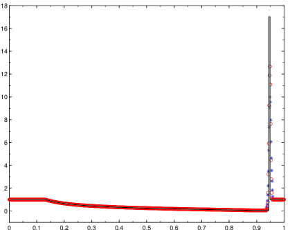
(a) $\rho$

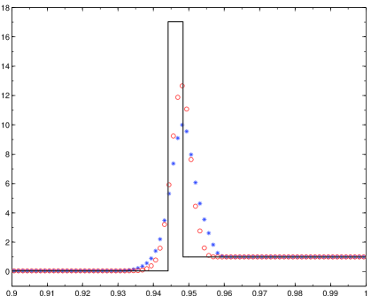
(b) Close-up of $\rho$

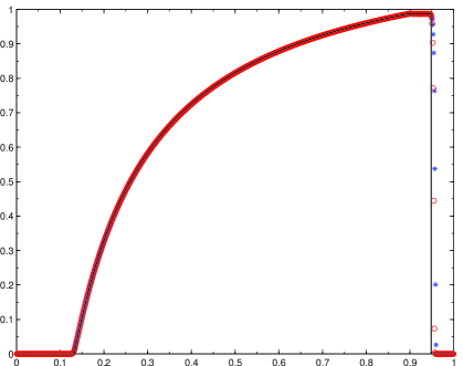
(c) $v_{1}$

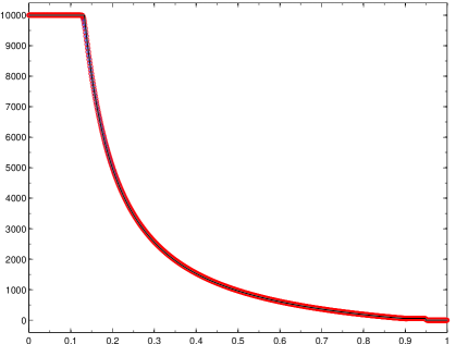
(d) $p$

Figure 4.1: Example 4.2: The density $\rho$ and its close-up, the velocity $v_{1}$, and the pressure $p$ at $t=0.45$ obtained by using PCPFDWENO5 (“$\ast$”) and PCPFDWENO9 (“$\circ$”) with 800 uniform cells.

Fig. 4.1 displays the numerical results at $t=0.45$ obtained by using PCPFDWENO5 (“$\ast$”) and PCPFDWENO9 (“$\circ$”) with 800 uniform cells within the domain $[0,1]$, where the solid line denotes the exact solution. It can be seen that PCPFDWENO9 exhibits better resolution than PCPFDWENO5, and they can well capture the wave configuration except for the extremely narrow region between the contact discontinuity and the shock wave. The main reason is that the region between the shock wave and the contact discontinuity is extremely narrow (its width at $t=0.45$ is about 0.00424) so that it can not be well resolved with 800 uniform cells. At the resolution of 800 uniform cells, the maximal densities for PCPFDWENO5 and PCPFDWENO9 within the above narrow region are about 58.7% and 74.4% of the analytic value, respectively.

Example 4.3 (Blast wave interaction)

This is an initial-boundary-value problem for the 1D RHD equations (3.1) and has been studied in [33, 58]. The same initial setup is considered here. The adiabatic index $\Gamma$ is taken as $1.4$, the initial data are taken as follows

$$\mbox{\boldmath\small$V$}(x,0)=\begin{cases}(1,0,1000)^{T},\ \ &0<x<0.1,\\ (1,0,0.01)^{T},\ \ &0.1<x<0.9,\\ (1,0,100)^{T},\ \ &0.9<x<1,\end{cases}$$ (4.2)

and outflow boundary conditions are specified at the two ends of the unit interval $[0,1]$. This is also a very severe test since it contains the most challenging one-dimensional relativistic wave configuration, e.g., strong relativistic shock waves, and interaction between blast waves in a narrow region, etc.

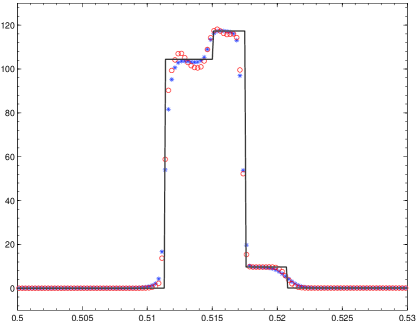
(a) $\rho$

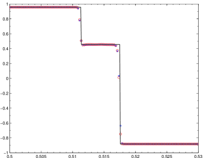
(b) $v_{1}$

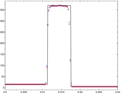
(c) $p$

(d) $e$

Figure 4.2: Example 4.3: Close-up of the numerical solutions at $t=0.43$ obtained by using PCPFDWENO5 (“$\ast$”) and PCPFDWENO9 (“$\circ$”) with 4000 uniform cells. The solid lines denote the exact solutions.

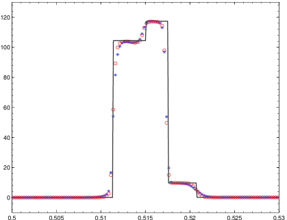
(a) $\rho$

(b) $v_{1}$

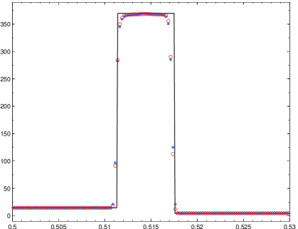
(c) $p$

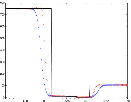
(d) $e$

Figure 4.3: Same as Fig. 4.2, except for PCPFDWENO9 (“$\circ$”) with a monotonicity-preserving limiter.

Fig. 4.2 gives close-up of the solutions at $t=0.43$ obtained by using PCPFDWENO5 (“$\ast$”) and PCPFDWENO9 (“$\circ$”) with 4000 uniform cells within the domain $[0,1]$. It is found that the solutions at $t=0.43$ within the interval $[0.5,0.53]$ consists two shock waves and two contact discontinuities since both initial discontinuities evolve and both blast waves collide each other; and compared to the GRP scheme in [58], both schemes can well resolve those discontinuities and clearly capture the complex relativistic wave configuration, but PCPFDWENO9 exhibits better resolution than PCPFDWENO5 except for slight overshoot and undershoot of the rest-mass density between the left shock and the contact discontinuity. The overshoot and undershoot may be suppressed by using the monotonicity-preserving limiter in [2], see Fig. 4.3.

Example 4.4 (Shock heating problem)

The last 1D test is to solve the shock heating problem, see [3], by using PCPFDWENO5 and PCPFDWENO9. The computational domain $[0,1]$ with a reflecting boundary at the right end is initially filled with a cold gas (the specific internal energy is taken as 0.0001). The gas has an unit rest-mass density, the adiabatic index $\Gamma$ of $4/3$, and the velocity $v_{0}$ of $1-10^{-10}$, When the initial gas moves toward to the reflecting boundary, the gas is compressed and heated as the kinetic energy is converted into the internal energy. After then, a reflected strong shock wave is formed and propagate to the left with the speed $v_{s}={(\Gamma-1)W_{0}|v_{0}|}/{(W_{0}+1)}$, where $W_{0}=(1-v_{0}^{2})^{-1/2}$ is about 70710.675. Behind the reflected shock wave, the gas is at rest and has a specific internal energy of $W_{0}-1$ due to the energy conservation across the shock wave. The compression ratio $\sigma$ across the relativistic shock wave

$$\sigma=\frac{\Gamma+1}{\Gamma-1}+\frac{\Gamma}{\Gamma-1}(W_{0}-1)\approx 282845.7,$$

grows linearly with the Lorentz factor $W_{0}$ and towards to infinite as the inflowing gas velocity approaches to speed of light. It is worth noting that the compression ratio across the shock wave in the non-relativistic case is always bounded by ${(\Gamma+1)}/{(\Gamma-1)}$.

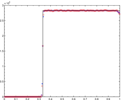
(a) $\rho$

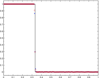
(b) $u$

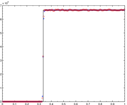
(c) $p$

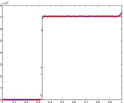
(d) $e$

Figure 4.4: Example 4.4: The density $\rho$, the velocity $v_{1}$, the pressure $p$, and the internal energy $e$ at $t=2$ obtained by using PCPFDWENO5 (“$\ast$”) and PCPFDWENO9 (“$\circ$”) with 200 uniform cells. The solid lines denote the exact solutions.

Fig. 4.4 displays the numerical solutions at $t=2$ obtained by using PCPFDWENO5 (“$\ast$”) and PCPFDWENO9 (“$\circ$”) with 200 uniform cells. It shows that both schemes exhibit good robustness for this ultra-relativistic problem and good resolution for the strong shock wave, even though there exist slight oscillations in the rest-mass density and the internal energy behind the shock wave as well as well-known wall-heating phenomenon near the reflecting boundary $x=1$. Similar to Example 4.3, those small oscillations can also be efficiently alleviated by using the monotonicity-preserving limiter [2]. To save the paper space, the results are not presented here.

Besides the flux limiter in Section 3.1.1, we have also tried to extend the parametrized flux limiter [56, 29, 54] to the 1D RHD equations (3.1), the numerical results show that the parametrized flux limiter is less restrictive on the CFL number in preserving high order accuracy and has slightly better resolution for Example 4.2 than the flux limiter in Section 3.1.1.

Example 4.5 (2D Riemann problem)

The non-relativistic 2D RPs are theoretically studied for the first time in [68]. After then, the 2D RPs become benchmark tests for verifying the accuracy and resolution of numerical schemes, see [45, 28, 17, 52, 50, 59].

Initial data of two RPs of 2D RHD equations (3.15) considered here comprise four different constant states in the unit square $\Omega=[0,1]\times[0,1]$, while initial discontinuities parallel to both coordinate axes respectively.

The initial data of the first RP are

$$\mbox{\boldmath\small$V$}({x},{y},0)=\begin{cases}(0.1,0,0,0.01)^{T},&x>0.5,y>0.5,\\ (0.1,0.99,0,1)^{T},&x<0.5,y>0.5,\\ (0.5,0,0,1)^{T},&x<0.5,y<0.5,\\ (0.1,0,0.99,1)^{T},&x>0.5,y<0.5,\end{cases}$$

where both the left and bottom discontinuities are contact discontinuities with a jump in the transverse velocity, while both the right and top discontinuities are not simple waves. Note that this test is different from the case in [59].

Fig. 4.5 gives the contours of the density logarithm $\ln\rho$ at time $t=0.4$ obtained by using PCPFDWENO5 and PCPFDWENO9 with several different mesh resolutions. It is found that four initial discontinuities interact each other and form two reflected curved shock waves, an elongated jet-like spike, which is approximately between two points (0.7,0.7) and (0.9,0.9) on the diagonal $x=y$ when $t=0.4$, and a complex mushroom structure starting from the point (0.5,0.5) respectively and expanding to the bottom-left region; both PCPFDWENO5 and PCPFDWENO9 well capture these complex wave configuration, and it is obvious that with the same mesh of $400\times 400$ uniform cells, PCPFDWENO9 gets better resolution of discontinuities than PCPFDWENO5, and the solutions obtained by PCPFDWENO9 with the mesh of $800\times 800$ uniform cells are comparable to those obtained by PCPFDWENO5 with a finer mesh of $1200\times 1200$ uniform cells. For a further comparison, the rest-mass densities are plotted along the line $y=x$ and $y=1$, see Fig. 4.6. Those plots validate the above observation.

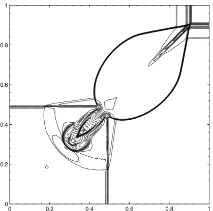
(a) ${\tt PCPFDWENO5}$ with $400\times 400$ uniform cells

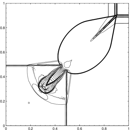
(b) ${\tt PCPFDWENO9}$ with $400\times 400$ uniform cells

(c) ${\tt PCPFDWENO5}$ with $1200\times 1200$ uniform cells

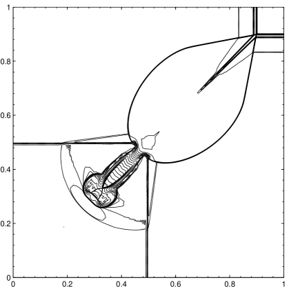
(d) ${\tt PCPFDWENO9}$ with $800\times 800$ uniform cells

Figure 4.5: The first 2D RP in Example 4.5: The contours of the density logarithm $\ln\rho$ at $t=0.4$ within the domain $[0,1]\times[0,1]$ obtained by using PCPFDWENO5 and PCPFDWENO9 (25 equally spaced contour lines from $-6$ to $1.9$).

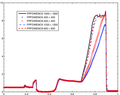
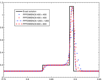
Figure 4.6: Same as Fig. 4.5, except for $\rho$ along the line $y=x$ within the scaled interval $[0,1]$ (left) and $\rho$ along the line $y=1$ within the closed interval $[0.75,0.95]$ (right).

The initial data of the second 2D RP are

$$\mbox{\boldmath\small$V$}({x},{y},0)=\begin{cases}(0.1,0,0,20)^{T},&x>0.5,y>0.5,\\ (0.00414329639576,0.9946418833556542,0,0.05)^{T},&x<0.5,y>0.5,\\ (0.01,0,0,0.05)^{T},&x<0.5,y<0.5,\\ (0.00414329639576,0,0.9946418833556542,0.05)^{T},&x>0.5,y<0.5,\end{cases}$$

where both the left and bottom discontinuities are contact discontinuities while both the top and right are shock waves with the speed of $-0.66525606186639$. As the time increases, the maximal value of the fluid velocity may be very close to the speed of light.

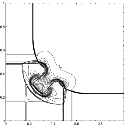
(a) ${\tt PCPFDWENO5}$

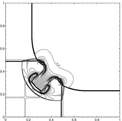
(b) ${\tt PCPFDWENO9}$

Figure 4.7: The second 2D RP in Example 4.5: The contours of the density logarithm $\ln\rho$ at $t=0.4$ within the domain $[0,1]\times[0,1]$ obtained by using PCPFDWENO5 and PCPFDWENO9 with $400\times 400$ uniform cells (25 equally spaced contour lines from $-8$ to $-2.3$).

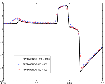
Figure 4.8: Same as Fig. 4.7, except for $\ln\rho$ along the line $y=x$ within the scaled interval $[0,1]$.

Fig. 4.7 displays the contours of the density logarithm $\ln\rho$ at time $t=0.4$ within the unit square $[0,1]\times[0,1]$ obtained by using PCPFDWENO5 and PCPFDWENO9 with the mesh of $400\times 400$ uniform cells. It is seen that the interaction of four initial discontinuities leads to the distortion of both initial shock wave and the formation of a “mushroom cloud” starting from the point $(0.5,0.5)$ and expanding to the left bottom region, and the present schemes have good performance and strong robustness in such ultra-relativistic flow simulation, in which the fluid velocity reachs 0.9998458 locally, or the Lorentz factor may be not lesser than 56.95. Plots of $\ln\rho$ along the line $y=x$ in Fig. 4.8 further show that PCPFDWENO9 captures the structure better than PCPFDWENO5.

Example 4.6 (Forward facing step problem)

The forward facing step problem was first introduced by Emery [12], has been widely used to test the non-relativistic hydrodynamic codes, e.g. [4], and extended to the ideal relativistic fluid, see [30, 61].

The same setup as in [61] is used here. The wind tunnel is located in the domain $[0,3]\times[0,1]$ and contains a forward facing step with a height of $0.2$, which starts from $x=0.6$ and continues along the length of the tunnel. Initially it is filled with an ideal gas with the density of 1.4, the velocity of 0.999, the Mach number of 3, and the adiabatic index of $1.4$. The reflective boundary conditions are specified on the walls of the tunnel, while the inflow and outflow boundary conditions are specified at two ends of the tunnel ($x=0$ and 3). Due to the forward facing step, the bow shock wave is formed and then a Mach reflection happens at the top wall of the tunnel. Later, the reflected shock wave incidents to the step and then the regular reflection of the shock wave is caused and generates a second reflected curved shock wave. Moreover, the step corner (0.6,0.2) is the center of a rarefaction fan and hence a singular point of the flow. Although the time-evolution of the flow is similar to the non-relativistic case, see e.g. [4], the present test is much more difficult than the non-relativistic case because the bow shock wave has a much fast speed and there exist the large jumps in the density and the pressure and the ultra-relativistic regime where the Lorentz factor $W\gg 1$.

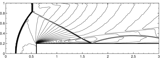
Figure 4.9: Example 4.6: The contours of the rest-mass density logarithm $\ln\rho$ at $t=4$ obtained by using PCPFDWENO5 (top) and PCPFDWENO9 (bottom) with $300\times 100$ uniform cells for the domain $[0,3]\times[0,1]$ (25 equally spaced contour lines from -0.86 to 4.64).

Fig. 4.9 gives the contours of the rest-mass density logarithm $\ln\rho$ at $t=4$ obtained by using the proposed PCPFDWENO5 and PCPFDWENO9 with $300\times 100$ uniform cells for the domain $[0,3]\times[0,1]$. Numerical results also show that across the Mach stem, the relative jumps $\Delta\rho={|\rho_{R}/\rho_{L}-1|}$ and $\Delta p={|p_{R}/p_{L}-1|}$ are about 61.33 and 5223.99, respectively, where the subscripts $L$ and $R$ denote corresponding left and right states. Comparing our results with those in [61], it can be seen that the flow structures are well obtained and the discontinuities, e.g. the bow and reflected shock waves and the Mach stem, are well captured with high resolution by using PCPFDWENO5 and PCPFDWENO9 without any artifical entropy fix around the step corner.

Example 4.7 (Axisymmetric relativistic jets)

The last 2D example is to simulate two high-speed relativistic jet flows by solving the axisymmetric RHD equations (3.19). The jet flows are ubiquitous in extragalactic radio sources associated with active galactic nuclei and the most compelling case for a special relativistic phenomenon. Since there are the ultra-relativistic region, strong relativistic shock wave and shear flow, and interface instabilities etc. in the high-speed jet flow, simulating successfully such jet flow can be a real challenge, see e.g. [36, 11, 35, 26].

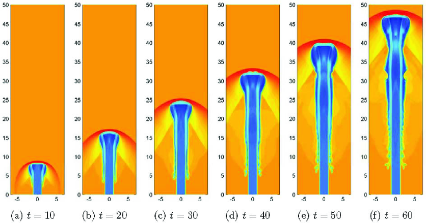
Figure 4.10: The hot A1 model in Example 4.7: Schlieren images of the rest-mass density logarithm $\ln\rho$ within the symmetrical domain $[-7,7]\times[0,50]$ at several different times obtained by using PCPFDWENO5 with $280\times 2000$ uniform cells.

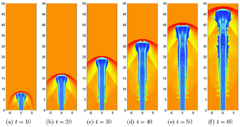
Figure 4.11: Same as Fig. 4.10 except for PCPFDWENO9.

The first test is a pressure-matched hot A1 model, see [35]. In this model, the classical beam Mach number $M_{b}$ is near the minimum Mach number $M^{\min}=v_{b}/\sqrt{\Gamma-1}$, the beam is moving at speed $v_{b}=0.99$, and relativistic effects from large beam internal energies are important and comparable to the effects from fluid velocity near the speed of light. Initially, the computational domain $[0,7]\times[0,50]$ in the $(r,z)$ plane is filled with a static uniform medium with unit rest-mass density with the adiabatic index of $4/3$. A light relativistic jet is injected in the $z$–direction through the inlet part ($r\leq 1$) of the bottom boundary ($z=0$) with a density of 0.01, a pressure equal to the ambient pressure, and a speed of $v_{b}$ or a Lorentz factor of 7.09. The relativistic Mach number $M_{r}:=M_{b}W/W_{s}$ is about 9.97, where $W_{s}=1/\sqrt{1-c_{s}^{2}}$ is the Lorentz factor associated with the local sound speed and $M_{b}=v_{b}/c_{s}$ is equal to 1.72. The symmetrical boundary condition is specified at $r=0$, the fixed inflow beam condition is specified on the nozzle $\{z=0,r\leq 1$}, while outflow boundary conditions are on other boundaries.

Figs. 4.10 and 4.11 display the schlieren images of the rest-mass density logarithm $\ln\rho$ within the domain $[-7,7]\times[0,50]$ at $t=10,20,30,40,50$ and 60 obtained by using PCPFDWENO5 and PCPFDWENO9 with $280\times 2000$ uniform cells respectively. Compared them to those in [35], it is found that the time evolution of a light, relativistic jet with large internal energy is well simulated by our schemes, and the Mach shock wave at the jet head is correctly and well captured during the whole simulation. Although the internal structure is almost completely lacked because of the pressure equilibrium between the beam and its surroundings, and the beam/cocoon interface of the hot jets is very stable against the growth of pinch instabilities that would evolve into internal shock waves, the proposed schemes still clearly resolve the beam/cocoon interface and the Kelvin-Helmholtz type instability at the beam/cocoon interface.

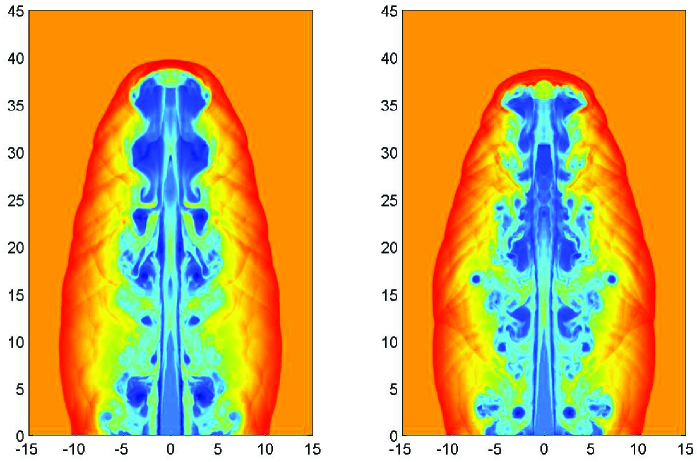
Figure 4.12: The highly supersonic jet test of Example 4.7: Schlieren images of the rest-mass density logarithm $\ln\rho$ at $t=100$ obtained by PCPFDWENO5 (left) and PCPFDWENO9 (right) on the mesh of $384\times 1152$ uniform cells.

The second test is the pressure-matched highly supersonic C2 jet model ($M_{b}\gg M^{\min}$, $\Gamma=5/3$, and $v_{b}=0.99$), see [35, 61]. Highly supersonic jets are also refered to cold models and the relativistic effects from large beam speeds dominate in C2 jet model so that there exist important differences between hot and cold relativistic jets.

The same setup as in [61] is used here within the computational domain $[0,15]\times[0,45]$ in the $(r,z)$ plane. The initial relativistic jet has the same rest-mass density and velocity as those in the above hot A1 model, but a higher Mach number of 6 (or corresponding relativistic Mach number of about 41.95) and a larger adiabatic index of $5/3$.

Fig. 4.12 shows the schlieren images of the rest-mass density logarithm $\ln\rho$ within the symmetrical domain $[-15,15]\times[0,45]$ at $t=100$ obtained by using PCPFDWENO5 and PCPFDWENO9 with $384\times 1152$ uniform cells. In our simulations, stable cocoons can be found in the early stages of the evolution, but these cocoons eventually evolve into large vortices producing turbulent structures, and the morphology and dynamics of the relativistic jets in Fig. 4.12 agree well with those obtained by using an adaptive mesh refinement RHD code in [61]. It is worth noting that the above-observed gross morphological features already found in non-relativistic calculations.

5 Conclusions

The paper developed ($2r-1$)th-order accurate finite difference WENO schemes for special RHD equations and proved that their solutions satisfied physical properties: the positivity of the rest-mass density and the pressure and the bounds of the velocity. The key contributions were that the convexity and some mathematical properties of the admissible state set ${\mathcal{G}}$ were proved and the concave function $q(\mbox{\boldmath\small$U$})$ with respect to the conservative vector $U$ was discovered. The schemes were built on the local Lax-Friedrich splitting, the WENO reconstruction, the physical-constraints-preserving flux limiter, and the high-order strong stability preserving time discretization. They were considered as formal extensions of positivity-preserving finite difference WENO schemes for the non-relativistic Euler equations [21]. However, developing physical-constraints-preserving methods for the RHD system became much more difficult than the non-relativistic case because of the strongly coupling between the RHD equations, no explicit expressions of the primitive variables $V$ and the flux vector $\mbox{\boldmath\small$F$}_{i}$ in terms of the conservative vector $U$, and one more physical constraint for the fluid velocity in addition to the positivity of the rest-mass density and the pressure, the non concavity of $p(\mbox{\boldmath\small$U$})$, which was a key ingredient to enforce the positivity-preserving property for the non-relativistic Euler equations.

Several numerical examples demonstrated accuracy, robustness, and effectiveness of the proposed physical-constraints-preserving schemes in solving relativistic problems with large Lorentz factor, or strong discontinuities, or low rest-mass density or pressure etc., which involved a 1D smooth problem, a 1D Riemann problem, a 1D blast wave interaction problem, and a 1D shock heating problem, two 2D Riemann problems, and a forward facing step problem and two axisymmetric jet flows in two dimensions.

Since the present physical-constraints-preserving limiting procedure was independent on the reconstruction in space, other high-order accurate reconstruction or interpolation could also be used to replace the WENO reconstruction. Moreover, it was possible that the analysis results and the limiting procedure etc. could be extended to develop high-order accurate physical-constraints-preserving finite volume schemes for the RHD equations.

References

- [1] D.S. Balsara, Riemann solver for relativistic hydrodynamics, J. Comput. Phys., 114 (1994), 284-297.
- [2] D.S. Balsara and C.-W. Shu, Monotonicity preserving weighted essentially non-oscillatory schemes with increasingly high-order of accuracy, J. Comput. Phys., 160 (2000), 405-452.
- [3] R.D. Blandford and C.F. McKee, Fluid dynamics of relativistic blast waves, Phys. Fluids, 19 (1976), 1130-1138.
- [4] G.X. Chen, H.Z. Tang and P.W. Zhang, Second-order accurate Godunov scheme for multicomponent flows on moving triangular meshes, J. Sci. Comput., 34 (2008), 64-86.
- [5] J. Cheng and C.-W. Shu, Positivity-preserving Lagrangian scheme for multi-material compressible flow, J. Comput. Phys., 257 (2014), 143-168.
- [6] A.J. Christlieb, Y. Liu, Q. Tang, and Z.F. Xu, Positivity-preserving finite difference WENO schemes with constrained transport for ideal magnetohydrodynamic equations, arXiv:1406.5098v2, 2014.
- [7] M. Cissoko, Detonation waves in relativistic hydrotlynamics, Phys. Rev. D, 45(1992), 1045-1052.
- [8] W.L. Dai and P.R. Woodward, An iterative Riemann solver for relativistic hydrodynamics, SIAM J. Sci. Stat. Comput., 18 (1997), 982-995.
- [9] A. Dolezal and S.S.M. Wong, Relativistic hydrodynamics and essentially non-oscillatory shock capturing schemes, J. Comput. Phys., 120 (1995), 266-277.
- [10] R. Donat, J.A. Font, J.M. Ibáñez, and A. Marquina, A flux-split algorithm applied to relativistic flows, J. Comput. Phys., 146 (1998), 58-81.
- [11] G.C. Duncan and P.A. Hughes, Simulations of relativistic extragalactic jets, Astrophys. J., 436 (1994), L119–L122.
- [12] A.F. Emery, An evaluation of several differencing methods for inviscid fluid flow problem, J. Comput. Phys., 2 (1968), 306-331.
- [13] F. Eulderink and G. Mellema, General relativistic hydrodynamics with a Roe solver, Astron. Astrophys. Suppl. S., 110 (1995), 587-623.
- [14] J.A. Font, Numerical hydrodynamics and magnetohydrodynamics in general relativity, Living Rev. Relativity, 11 (2008), 7.
- [15] G.A. Gerolymos, D. Sénéchal and I. Vallet, Very-high-order WENO schemes, J. Comput. Phys., 228 (2009), 8481-8524.
- [16] S. Gottlieb, D.J. Ketcheson and C.-W. Shu, High order strong stability preserving time discretizations, J. Sci. Comput., 38 (2009), 251-289.
- [17] E. Han, J.Q. Li and H.Z. Tang, Accuracy of the adaptive GRP scheme and the simulation of 2-D Riemann problems for compressible Euler equations, Commun. Comput. Phys., 10 (3) (2011), 577-606.
- [18] P. He, Numerical Simulations of Relativistic Hydrodynamics and Relativistic Magneto- hydrodynamics, Ph.D. thesis, School of Mathematical Sciences, Peking University, 2011.
- [19] P. He and H.Z. Tang, An adaptive moving mesh method for two-dimensional relativistic hydrodynamics, Commun. Comput. Phys., 11 (2012), 114-146.
- [20] P. He and H.Z. Tang, An adaptive moving mesh method for two-dimensional relativistic magnetohydrodynamics, Comput. & Fluids, 60 (2012), 1-20.
- [21] X.Y. Hu, N.A. Adams and C.-W. Shu, Positivity-preserving method for high-order conservative schemes solving compressible Euler equations, J. Comput. Phys., 242 (2013), 169-180.
- [22] P.A. Hughes, M.A. Miller and G.C. Duncan, Three-dimensional hydrodynamic simulations of relativistic extragalactic jets, Astrophys. J., 572 (2002), 713-728.
- [23] J.Ma. Ibán̈ez and J.Ma. Martí, Riemann solvers in relativistic astrophysics, J. Comput. Appl. Math., 109 (1999), 173-211.
- [24] G.-S. Jiang and C.-W. Shu, Efficient implementation of weighted ENO schemes, J. Comput. Phys., 126 (1996), 202-228.
- [25] Y. Jiang and Z.F. Xu, Parametrized maximum principle preserving limiter for finite difference WENO schemes solving convection-dominated diffusion equations, SIAM J. Sci. Comput., 35 (2013), A2524-A2553.
- [26] S.S. Komissarov and S.A.E.G. Falle, The large-scale structure of FR-II radio sources, Mon. Not. R. Astron. Soc., 297 (1998), 1087-1108.
- [27] M. Kunik, S. Qamar, and G. Warnecke, Kinetic schemes for the relativistic gas dynamics, Numer. Math., 97 (2004), 159-191.
- [28] P.D. Lax and X.D. Liu, Solution of two-dimensional Riemann problems of gas dynamics by positive schemes, SIAM J. Sci. Comput., 19 (1998), 319-340.
- [29] C. Liang and Z.F. Xu, Parametrized maximum principle preserving flux limiters for high-order schemes solving multi-dimensional scalar hyperbolic conservation laws, J. Sci. Comput., 58 (2014), 41-60.
- [30] A. Lucas-Serrano, J. A. Font, J. M. Ibáñez and and J.M. Martí, Assessment of a high-resolution central scheme for the solution of the relativistic hydrodynamics equations, Astron. Astrophys., 428 (2004), 703-715.
- [31] M.M. May and R.H. White, Hydrodynamic calculations of general-relativistic collapse, Phys. Rev., 141 (1966), 1232-1241.
- [32] M.M. May and R.H. White, Stellar dynamics and gravitational collapse, Methods Comput. Phys., 7 (1967), 219-258.
- [33] J.M. Martí and E. Müller, Extension of the piecewise parabolic method to one-dimensional relativistic hydrodynamics, J. Comput. Phys., 123 (1996), 1-14.
- [34] J.M. Martí and E. Müller, Numerical hydrodynamics in special relativity, Living Rev. Relativity, 6 (2003), 7.
- [35] J.M. Martí, E. Müller, J. A. Font, J. M. Ibáñez and A. Marquina, Morphology and dynamics of relativistic jets, Astrophys. J., 479 (1997), 151-163.
- [36] J.M. Martí, E. Müller and J. M. Ibáñez, Hydrodynamical simulations of relativistic jets, Astron. Astrophys., 281 (1994), L9-L12.
- [37] A. Mignone and G. Bodo, An HLLC Riemann solver for relativistic flows, I: hydrodynamics, Mon. Not. R. Astron. Soc., 364 (2005), 126-136.
- [38] A. Mignone, T. Plewa, and G. Bodo, The piecewise parabolic method for multidimensional relativistic fluid dynamics, Astrophys. J. Suppl. S., 160 (2005), 199-219.
- [39] S. Qamar and G. Warnecke, A high-order kinetic flux-splitting method for the relativistic magnetohydrodynamics, J. Comput. Phys., 205 (2005), 182-204.
- [40] S. Qamar and M. Yousaf, The space-time CESE method for solving special relativistic hydrodynamic equations, J. Comput. Phys., 231 (2012), 3928-3945.
- [41] J.M. Qiu and C.-W. Shu, Positivity preserving semi-Lagrangian discontinuous Galerkin formulation: theoretical analysis and application to the Vlasov-Poisson system, J. Comput. Phys., 230 (2011), 8386-8409.
- [42] D. Radice and L. Rezzolla, Discontinuous Galerkin methods for general-relativistic hydrodynamics: Formulation and application to spherically symmetric spacetimes, Phys. Rev. D, 84 (2011), 024010.
- [43] V. Schneider, U. Katscher, D.H. Rischke, B. Waldhauser, J.A. Maruhn and C.D. Munz, New algorithms for ultra-relativistic numerical hydrodynamics, J. Comput. Phys., 105 (1993), 92-107.
- [44] C.-W. Shu, High Order Weighted essentially nonoscillatory schemes for convection dominated problems, SIAM Rev., 51 (2009), 82-126.
- [45] C.W. Schulz-Rinne, J.P. Collins and H.M. Glaz, Numerical solution of the Riemann problem for two-dimensional gas dynamics, SIAM J. Sci. Comput., 14 (6)(1993), 1394-1414.
- [46] A. Tchekhovskoy, J.C. McKinney and R. Narayan, WHAM: a WENO-based general relativistic numerical scheme, I: hydrodynamics, Mon. Not. R. Astron. Soc., 379 (2007), 469-497.
- [47] C. Wang, X.X. Zhang, C.-W. Shu and J.G. Ning, Robust high-order discontinuous Galerkin schemes for two-dimensional gaseous detonations, J. Comput. Phys., 231 (2012), 653-665.
- [48] J.R. Wilson, Numerical study of fluid flow in a Kerr space, Astrophys. J., 173 (1972), 431-438.
- [49] J.R. Wilson and G.J. Mathews, Relativistic Numerical Hydrodynamics, Cambridge University Press, 2007.
- [50] K.L. Wu and H.Z. Tang, Finite volume local evolution Galerkin method for two-dimensional relativistic hydrodynamics, J. Comput. Phys., 256 (2014), 277-307.
- [51] K.L. Wu, Z.C. Yang and H.Z. Tang, A third-order accurate direct Eulerian GRP scheme for one-dimensional relativistic hydrodynamics, East Asian J. Appl. Math., 4 (2014), 95-131.
- [52] K.L. Wu, Z.C. Yang, and H.Z. Tang, A third-order accurate direct Eulerian GRP scheme for the Euler equations in gas dynamics, J. Comput. Phys., 264 (2014), 177-208.
- [53] Y.L. Xing, X.X Zhang and C.-W. Shu, Positivity-preserving high-order well-balanced discontinuous Galerkin methods for the shallow water equations, Adv. Water Resour., 33 (2010), 1476-1493.
- [54] T. Xiong, J.-M. Qiu, and Z.F. Xu, Parametrized positivity preserving flux limiters for the high order finite difference WENO scheme solving compressible Euler equations, arXiv:1403.0594.
- [55] T. Xiong, J.-M. Qiu, and Z.F. Xu, A parametrized maximum principle preserving flux limiter for finite difference RK-WENO schemes with applications in incompressible flows, J. Comput. Phys., 252 (2013), 310-331.
- [56] Z.F. Xu, Parametrized maximum principle preserving flux limiters for high order schemes solving hyperbolic conservation laws: one-dimensional scalar problem, Math. Comput., 83 (2014), 2213-2238.
- [57] J.Y. Yang, M.H. Chen, I.N. Tsai, and J.W. Chang, A kinetic beam scheme for relativistic gas dynamics, J. Comput. Phys., 136 (1997), 19-40.
- [58] Z.C. Yang, P. He, and H.Z. Tang, A direct Eulerian GRP scheme for relativistic hydrodynamics: one-dimensional case, J. Comput. Phys., 230 (2011),7964-7987.
- [59] Z.C. Yang and H.Z. Tang, A direct Eulerian GRP scheme for relativistic hydrodynamics: two-dimensional case, J. Comput. Phys., 231 (2012), 2116-2139.
- [60] L.D. Zanna and N. Bucciantini, An efficient shock-capturing central-type scheme for multidimensional relativistic flows, I: hydrodynamics, Astron. Astrophys., 390 (2002), 1177-1186.
- [61] W.Q. Zhang and A.I. Macfadyen, RAM: a relativistic adpative mesh refinement hydrodynamics code, Astrophys. J. Suppl. S., 164 (2006), 255-279.
- [62] X.X. Zhang and C.-W. Shu, On maximum-principle-satisfying high-order schemes for scalar conservation laws, J. Comput. Phys., 229 (2010), 3091-3120.
- [63] X.X. Zhang and C.-W. Shu, On positivity-preserving high-order discontinuous Galerkin schemes for compressible Euler equations on rectangular meshes, J. Comput. Phys., 229 (2010), 8918-8934.
- [64] X.X. Zhang and C.-W. Shu, Positivity-preserving high-order discontinuous Galerkin schemes for compressible Euler equations with source terms, J. Comput. Phys., 230 (2011), 1238-1248.
- [65] X.X. Zhang and C.-W. Shu, Maximum-principle-satisfying and positivity-preserving high-order schemes for conservation laws: survey and new developments, Proc. R. Soc. A, 467 (2011), 2752-2776.
- [66] X.X. Zhang and C.-W. Shu, Positivity-preserving high-order finite difference WENO schemes for compressible Euler equations, J. Comput. Phys., 231 (2012), 2245-2258.
- [67] X.X. Zhang, Y.H. Xia and C.-W. Shu, Maximum-principle-satisfying and positivity-preserving high-order discontinuous galerkin schemes for conservation laws on triangular meshes, J. Sci. Comput., 50 (2012), 29-62.
- [68] T. Zhang and Y.X. Zheng, Conjecture on the structure of solutions of the Riemann problem for two-dimensional gas dynamics systems, SIAM J. Math. Anal., 21 (1990), 593-630.
- [69] J. Zhao, P. He and H.Z. Tang, Steger-Warming flux vector splitting method for special relativistic hydrodynamics, Math. Meth. Appl. Sci., 37 (2014), 1003-1018.
- [70] J. Zhao and H.Z. Tang, Runge-Kutta discontinuous Galerkin methods with WENO limiter for the special relativistic hydrodynamics, J. Comput. Phys., 242 (2013), 138-168.