Temperature dependence of meson screening masses; a comparison of effective model with lattice QCD

Abstract:

Temperature dependence of pion and sigma-meson screening masses is evaluated by the Polyakov-loop extended Nambu–Jona-Lasinio model with the entanglement vertex (EPNJL model). We propose a practical way of calculating meson screening masses in the NJL-type effective models. The method based on the Pauli-Villars regularization solves the well-known difficulty that the evaluation of screening masses is not easy in the NJL-type effective models. The method is applied to analyze temperature dependence of pion screening masses calculated with state-of-the-art lattice simulations with success in reproducing the lattice QCD results. We predict the temperature dependence of pole mass by using EPNJL model.

1 Introduction

Meson masses are not only fundamental quantities of hadrons but also a key to know properties of quantum chromodynamics (QCD) vacuum. At finite temperature ($T$), we can define two kinds of meson masses, pole and screening mass. Meson pole masses are one of the possible observables in the heavy ion collisions. Screening masses of light mesons are essential for the range of the nuclear force. Accordingly, it is necessary to construct the effective model for calculating pole and screening mass simultaneously.

In lattice QCD(LQCD), meson pole (screening) masses are calculated from the exponential decay of temporal (spatial) mesonic correlation functions. LQCD simulations are more difficult for pole masses than for screening masses, since the lattice size is smaller in the time direction than in the spatial direction. This situation becomes more serious as $T$ increases. For this reason, meson screening masses were calculated in most of the LQCD simulations. Recently, a state-of-the-art calculation was done for meson screening masses in a wide range of $T<800$ MeV [1]

Constructing the effective model is an approach complementary to the first-principle LQCD simulation. In contrast to LQCD simulations, meson pole masses are extensively investigated at finite $T$ by the Nambu–Jona-Lasinio (NJL) model [2, 3], the Polyakov-loop extended Nambu–Jona-Lasinio (PNJL) model [4]. However, only a few trials were made so far for the evaluation of meson screening masses $M_{\xi,{\rm scr}}$ [2, 3]; here $\xi$ means a species of mesons. The model calculations have essentially two problems. One problem is that the NJL-type models are nonrenormalizable and hence the regularization is needed in the model calculations. The regularization commonly used is the three-dimensional momentum cutoff. The momentum cutoff breaks Lorentz and translational invariance, thereby the spatial correlation function $\eta_{\xi\xi}(r)$ has an unphysical oscillation [3]. This makes the determination of $M_{\xi,{\rm scr}}$ quite difficult, since $M_{\xi,{\rm scr}}$ is defined from the exponential decay of $\eta_{\xi\xi}(r)$ at large distance ($r$):

$$M_{\xi,{\rm scr}}=-\lim_{r\rightarrow\infty}\frac{d\ln{\eta_{\xi\xi}(r)}}{dr}.$$ (1)

Another problem is the feasibility of numerical calculations. In the model approach, $\eta_{\xi\xi}(r)$ is first obtained in the momentum ($\vec{q}$) representation $\chi_{\xi\xi}(0,\vec{q}^{2})$. In the Fourier transformation to the coordinate representation ($r=|\vec{x}|$),

$$\eta_{\xi\xi}(r)=\int\frac{d^{3}q}{(2\pi)^{3}}\chi_{\xi\xi}(0,\vec{q}^{2})e^{i\vec{q}\cdot\vec{x}}=\frac{1}{4\pi^{2}ir}\int^{\infty}_{-\infty}d\tilde{q}\hskip 4.30554pt\tilde{q}\chi_{\xi\xi}(0,\tilde{q}^{2})e^{i\tilde{q}r}\hskip 4.30554pt.$$ (2)

The integrand is slowly damping and highly oscillating particularly at large $r$ where $M_{\xi,{\rm scr}}$ is defined. This requires heavy numerical calculations. It was then proposed that the contour integral was made in the complex-$\tilde{q}$ plane [3]. However, the contour integral is still hard to do because of the presence of the temperature cuts in the vicinity of the real axis [3]; see the left panel of Fig. 1, where note that $\epsilon$ is an infinitesimal quantity.

In this talk, we propose a new formalism for calculating screening mass and discuss the possibility of the prediction for pole mass from screening mass by using effective model. This talk is based on the paper [5].

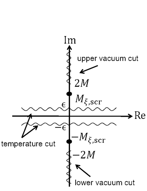
Fig. 1: Singularities of $\chi_{\xi\xi}(0,\tilde{q}^{2})$ in the complex-$\tilde{q}$ plane based on the previous formulation [3] (left) and the present formulation (right). Cuts are denoted by the wavy lines and poles by the points.

2 Formalism

The Lagrangian density of the two-flavor EPNJL model [6] is defined as

$${\cal L}={\bar{q}}(i\gamma_{\nu}D^{\nu}-m_{0})q+G_{\rm s}(\Phi)[({\bar{q}}q)^{2}+({\bar{q}}i\gamma_{5}{\vec{\tau}}q)^{2}]-{\cal U}(\Phi[A],{\bar{\Phi}}[A],T)$$ (3)

with the quark field $q$, the current quark mass $m_{0}$ and the isospin matrix ${\vec{\tau}}$. The coupling constant $G_{\rm s}(\Phi)$ of the four-quark interaction depends on the Polyakov loop $\Phi$ as

$$G_{\rm s}(\Phi)=G_{\rm s}\left[1-\alpha_{1}\Phi{\bar{\Phi}}-\alpha_{2}\left(\Phi^{3}+{\bar{\Phi}}^{3}\right)\right],$$ (4)

where $D^{\nu}=\partial^{\nu}+iA^{\nu}$ with $A^{\nu}=\delta^{\nu}_{0}g(A^{0})_{a}{\lambda_{a}/2}=-\delta^{\nu}_{0}ig(A_{4})_{a}{\lambda_{a}/2}$ for the gauge field $A^{\nu}_{a}$, the Gell-Mann matrix $\lambda_{a}$ and the gauge coupling $g$. When $\alpha_{1}=\alpha_{2}=0$, the EPNJL model is reduced to the PNJL model [4].

In the EPNJL model, only the time component of $A_{\mu}$ is treated as a homogeneous and static background field, which is governed by the Polyakov-loop potential  $\mathcal{U}$. The Polyakov loop $\Phi$ and its conjugate ${\bar{\Phi}}$ are then obtained in the Polyakov gauge by

$$\Phi ={1\over{3}}{\rm tr}_{\rm c}(L),~{}~{}~{}~{}~{}{\bar{\Phi}}={1\over{3}}{\rm tr}_{\rm c}({L^{*}})$$ (5)

with $L=\exp[iA_{4}/T]=\exp[i{\rm diag}(A_{4}^{11},A_{4}^{22},A_{4}^{33})/T]$ for the classical variables $A_{4}^{ii}$ satisfying that $A_{4}^{11}+A_{4}^{22}+A_{4}^{33}=0$. For zero chemical potential, $\Phi$ equals to ${\bar{\Phi}}$. Hence it is possible to set $A^{33}_{4}=0$ and determine the others as $A^{22}_{4}=-A^{11}_{4}={\rm cos}^{-1}(\frac{3\Phi-1}{2})T$. We use the logarithm-type Polyakov-loop potential $\mathcal{U}$ of Ref. [7], but refit the parameter $T_{0}$ to reproduce the chiral phase transition temperature $T_{c}$ because the original value of $T_{0}$ is set to $270$ MeV which is the deconfinement transition temperature in the pure gauge limit.

Making the mean field approximation to (3) and the path integral over the quark field, one can get the thermodynamic potential (per unit volume) as

$$\Omega=U_{\rm M}+{\cal U}-2N_{\rm f}\int\frac{d^{3}p}{(2\pi)^{3}}\Bigl{[}3E_{p} + \frac{1}{\beta}\ln~{}[1+3(\Phi+{\bar{\Phi}}e^{-\beta E_{p}})e^{-\beta E_{p}}+e^{-3\beta E_{p}}]$$

$$+ \frac{1}{\beta}\ln~{}[1+3({\bar{\Phi}}+{\Phi e^{-\beta E_{p}}})e^{-\beta E_{p}}+e^{-3\beta E_{p}}]\Bigl{]}$$

with $\beta=1/T$, $M=m_{0}-2G_{\rm s}(\Phi)\sigma$, $E_{p}=\sqrt{\vec{p}^{2}+M^{2}}$, and $U_{\rm M}=G_{\rm s}(\Phi)\sigma^{2}$. Here, $\sigma$ means chiral condensate $\langle\bar{q}q\rangle$. $N_{\rm f}$ is the number of flavors. We determine the mean field variables ($X=\sigma,\Phi,\bar{\Phi}$) from the stationary conditions for $\Omega$,

$$\frac{\partial\Omega}{\partial X}=0~{}.$$ (7)

Since the momentum integral of (LABEL:PNJL-Omega) diverges, we use the Pauli–Villars (PV) regularization [3, 8]. In the scheme, the integral $I(M,q)$ is regularized as

$$I^{\rm reg}(M,q)=\sum_{\alpha=0}^{2}C_{\alpha}I(M_{\alpha},q),$$ (8)

where $M_{0}=M$ and $M_{\alpha}~{}(\alpha\geq 1)$ are masses of auxiliary particles. The parameters $M_{\alpha}$ and $C_{\alpha}$ should satisfy the condition $\sum_{\alpha=0}^{2}C_{\alpha}=\sum_{\alpha=0}^{2}C_{\alpha}M_{\alpha}^{2}=0$. We then assume $(C_{0},C_{1},C_{2})=(1,1,-2)$ and $(M_{1}^{2},M_{2}^{2})=(M^{2}+2\Lambda^{2},M^{2}+\Lambda^{2})$. We keep the parameter $\Lambda$ finite even after the subtraction (8), since the present model is nonrenormalizable. The parameters taken are $m_{0}=6.3$ MeV, $G_{\rm s}=5.0$ GeV^-2 and $\Lambda=0.768$ GeV. This parameter set reproduces the pion decay constant $f_{\pi}=93.3$ MeV and the pion mass $M_{\pi}=138$ MeV at vacuum.

We derive the equations for pion and sigma-meson masses, following Ref [4]. We consider currents with the same quantum number as pion ($P$) and sigma-meson ($S$),

$${J_{P}}^{a}(x)=\bar{q}(x)i\gamma_{5}\tau^{a}q(x)~{},~{}{J_{S}}(x)=\bar{q}(x)q(x)-\langle\bar{q}(x)q(x)\rangle.$$ (9)

The Fourier transform of the mesonic correlation function $\eta_{\xi\xi}(x)\equiv\langle 0|T\left(J_{\xi}(x)J^{\dagger}_{\xi}(0)\right)|0\rangle$ is

$$\chi_{\xi\xi}(q^{2})=i\int d^{4}x~{}e^{iq\cdot x}\langle 0|{\rm T}\left(J_{\xi}(x)J^{\dagger}_{\xi}(0)\right)|0\rangle,$$ (10)

where $\xi=P^{a}$ for pion and $S$ for sigma meson and ${\rm T}$ stands for the time-ordered product. Using the random-phase (ring) approximation, one can obtain $\chi_{\xi\xi}$ as follows,

$$\chi_{\xi\xi} = \frac{\Pi_{\xi\xi}}{1-2G_{\rm s}(\Phi)\Pi_{\xi\xi}},$$ (11)

where the one-loop polarization function $\Pi_{\xi\xi}$ is explicitly obtained by

$$\Pi_{SS}=2iN_{\rm f}[I_{1}+I_{2}-(q^{2}-4M^{2})I_{3}]~{},~{}\Pi_{PP}=2iN_{\rm f}[I_{1}+I_{2}-q^{2}I_{3}],$$ (12)

with

$$I_{1} = \int{d^{4}p\over{(2\pi)^{4}}}{\rm tr_{c}}\Bigl{[}{1\over{p^{\prime 2}-M^{2}}}\Bigr{]},~{}~{}I_{2}=\int{d^{4}p\over{(2\pi)^{4}}}{\rm tr_{c}}\Bigl{[}{1\over{(p^{\prime}+q)^{2}-M^{2}}}\Bigr{]},$$ (13)

$$I_{3} = \int{d^{4}p\over{(2\pi)^{4}}}{\rm tr_{c}}\Bigl{[}{1\over{\{(p^{\prime}+q)^{2}-M^{2}\}(p^{\prime 2}-M^{2})}}\Bigr{]},$$ (14)

Here, $q^{2}=q_{0}^{2}-\vec{q}^{2}$ and $p^{\prime}=(p_{0}+iA_{4},\vec{p})$. ${\rm tr}_{\rm c}$ means the trace of color matrix. For finite $T$, the corresponding equations are obtained by the replacement

$$p_{0} \to i\omega_{l}=i(2l+1)\pi T~{},~{}\int\frac{d^{4}p}{(2\pi)^{4}}\to iT\sum_{l=-\infty}^{\infty}\int\frac{d^{3}p}{(2\pi)^{3}}.$$ (15)

The meson pole mass $M_{\xi,{\rm pole}}$ is a pole of $\chi_{\xi\xi}(q_{0}^{2},\vec{q}^{2})$. Taking the rest frame $q=(q_{0},\vec{0})$ for convenience, one can get the equation for $M_{\xi,{\rm pole}}$ as

$$\big{[}1-2G_{\rm s}(\Phi)\Pi_{\xi\xi}(q_{0}^{2},0)\big{]}\big{|}_{q_{0}=M_{\xi,{\rm pole}}}=0.$$ (16)

The method of calculating meson pole masses is well established in the PNJL model [4].

The meson screening mass $M_{\xi,{\rm scr}}$ defined with (1) is obtained by making the Fourier transform of $\chi_{\xi\xi}(0,\tilde{q}^{2})$ as shown in (2). In the previous formalism [3], however, the procedure requires heavy numerical calculations in the $I_{3}^{\rm reg}$ part, as shown below, where $I_{3}^{\rm reg}$ means a function after the PV regularization. Taking the $l$ summation before the $p$ integral in (15), one can describe $I_{3}^{\rm reg}(0,\tilde{q}^{2})$ as the sum of the vacuum and temperature parts, $I_{3,{\rm vac}}^{\rm reg}$ and $I_{3,{\rm tem}}^{\rm reg}$, defined by

$$I_{3,{\rm vac}}^{\rm reg}(0,\tilde{q}^{2}) = \frac{-iN_{c}}{16\pi^{2}}\sum_{\alpha=0}^{2}C_{\alpha}\left[\ln{M_{\alpha}^{2}}+f_{\rm vac}\left(\frac{2M_{\alpha}}{\tilde{q}}\right)\right],~{}~{}~{}$$ (17)

$$I_{3,{\rm tem}}^{\rm reg}(0,\tilde{q}^{2}) = \frac{iN_{c}}{16\pi^{2}}\sum_{\alpha=0}^{2}C_{\alpha}\int_{0}^{\infty}d|\vec{p}|~{}f_{\rm tem}(|\vec{p}|,\tilde{q})\left[F^{+}(E_{p})+F^{-}(E_{p})\right],~{}~{}~{}~{}~{}~{}$$ (18)

$$f_{\rm vac}(x) = \sqrt{1+x^{2}}\ln{\left(\frac{\sqrt{1+x^{2}}+1}{\sqrt{1+x^{2}}-1}\right)}~{},~{}f_{\rm tem}(|\vec{p}|,\tilde{q})=\frac{1}{E_{p}}\frac{|\vec{p}|}{\tilde{q}}\ln{\left(\frac{(\tilde{q}-2|\vec{p}|)^{2}+\epsilon^{2}}{(\tilde{q}+2|\vec{p}|)^{2}+\epsilon^{2}}\right)},\hskip 17.22217pt$$ (19)

where $F_{\pm}$ are the Fermi distribution functions. $F_{\pm}$ are defined as

$$F^{\pm}(E_{p})=\frac{1}{N_{c}}\sum_{i=1}^{N_{c}}{1\over{e^{(E_{p}\pm iA^{ii}_{4})/T}+1}}.$$ (20)

In (19), the $\epsilon^{2}$ term is added to make the $|\vec{p}|$ integral well defined at $\tilde{q}=\pm 2|\vec{p}|$, but this requires the limit of $\epsilon\to 0$.

As shown in the left panel of Fig. 1, $f_{\rm vac}({2M_{\alpha}}/{\tilde{q}})$ and $f_{\rm tem}(|\vec{p}|,\tilde{q})$ have the vacuum and temperature cuts in the complex $\tilde{q}$ plane, respectively. In (2), the cuts contribute to the $\tilde{q}$ integral in addition to the pole at $\tilde{q}=iM_{\xi,{\rm scr}}$ defined by

$$\big{[}1-2G_{\rm s}(\Phi)\Pi_{\xi\xi}(0,\tilde{q}^{2})\big{]}\big{|}_{\tilde{q}=iM_{\xi,{\rm scr}}}=0.$$ (21)

It is not easy to evaluate the temperature-cut contribution, since in (2) the integrand is slowly damping and highly oscillating with $\tilde{q}$ near the real axis in the complex $\tilde{q}$ plane. Furthermore we have to take the limit of $\epsilon\to 0$ finally. In order to avoid this problem, we integrate about $p$ in (15) before taking Matsubara summation $\sum_{l}$. Consequently, we can rewrite $I_{3}^{\rm reg}$ as an infinite series of analytic function,

$$I_{3}^{\rm reg}(0,\tilde{q}^{2})={iT\over{4\pi\tilde{q}}}\sum_{i=1}^{N_{c}}\sum_{l=-\infty}^{\infty}\sum_{\alpha=0}^{2}C_{\alpha}\sin^{-1}{\left({{\tilde{q}\over{2}}\over{\sqrt{{\tilde{q}^{2}\over{4}}+M_{i,l,\alpha}^{2}}}}\right)},$$ (22)

where

$$M_{i,l,\alpha}(T)=\sqrt{M_{\alpha}^{2}+\{(2l+1)\pi T+A_{4}^{ii}\}^{2}}.$$ (23)

We have numerically checked that the convergence of $l$ summation is quite fast in (22). Each term of $I_{3}^{\rm reg}(0,\tilde{q}^{2})$ has only two cuts starting from $\pm 2iM_{i,l,\alpha}$ on the imaginary axis in the complex $\tilde{q}$ plane. The cuts are shown in the right panel of Fig. 1. The lowest branch point is $\tilde{q}=2iM_{i=1,l=0,\alpha=0}$. Hence $2M_{i=1,l=0,\alpha=0}$ is regarded as “threshold mass” in the sense that the meson screening-mass spectrum becomes continuous above the point.

If $M_{\xi,{\rm scr}}<2M_{i=1,l=0,\alpha=0}$, the pole at $\tilde{q}=iM_{\xi,{\rm scr}}$ is well isolated from the cut. Hence one can take the contour (A$\to$B$\to$C$\to$D$\to$A) shown in the right panel of Fig. 1. The $\tilde{q}$ integral of $\tilde{q}\chi_{\xi\xi}(0,\tilde{q}^{2})e^{i\tilde{q}r}$ on the real axis in (2) is then obtained from the residue at the pole and the line integral from point C to point D. The former behaves as $\exp[-M_{\xi,{\rm scr}}r]/r$ at large $r$ and the latter as $\exp[{-2M_{i=1,l=0,\alpha=0}}r]/r$. The behavior of $\eta_{\xi\xi}(r)$ at large $r$ is thus determined by the pole. One can then determine the screening mass from the location of the pole in the complex-$\tilde{q}$ plane without making the $\tilde{q}$ integral. In the high-$T$ limit, the condition tends to $M_{\xi,{\rm scr}}<2\pi T$.

3 Numerical Results

The pion screening mass $M_{\pi,{\rm scr}}$ obtained by state-of-the-art 2+1 flavor LQCD simulations [1] is now analyzed by the present two-flavor EPNJL model simply, since pion is composed of $u$ and $d$ quarks. This is a quantitative analysis, because the finite lattice-spacing effect is not negligible in the simulations. The chiral transition temperature is evaluated as $T_{c}=196~{}{\rm MeV}$ in the simulations [1], although it becomes $T_{c}=154\pm 9~{}{\rm MeV}$ in finer 2+1-flavor LQCD simulations [9] close to the continuum limit. Therefore, we rescale the LQCD results of Ref. [1] with multiplying them by the factor $154/196$ to reproduce $T_{c}=154\pm 9~{}{\rm MeV}$. The model parameters, $m_{0}$ and $T_{0}$, are refitted to reproduce the rescaled 2+1 flavor LQCD data, i.e., $M_{\pi}=175~{}{\rm MeV}$ at vacuum and $T_{c}=154\pm 9~{}{\rm MeV}$; the resulting values are $m_{0}=10.3~{}{\rm MeV}$ and $T_{0}=156~{}{\rm MeV}$. The variation of $m_{0}$ from the original value $6.3$ to $10.3~{}{\rm MeV}$ little changes $\sigma$ and $\Phi$.

As shown in Fig. 3, the $M_{\pi,{\rm scr}}$ calculated with the EPNJL model (solid line) well reproduces the LQCD result (open circles), when $\alpha_{1}=\alpha_{2}=0.31$. In the PNJL model with $\alpha_{1}=\alpha_{2}=0$, the model result (dotted line) largely underestimates the LQCD result, indicating that the entanglement is important. The dashed line denotes the sigma-meson screening mass $M_{\sigma,{\rm scr}}$ obtained by the EPNJL model with $\alpha_{1}=\alpha_{2}=0.31$. The solid and dashed lines are lower than the threshold mass $2M_{i=1,l=0,\alpha=0}$ (dot-dashed line). This guarantees that the $M_{\pi,{\rm scr}}$ and $M_{\sigma,{\rm scr}}$ determined from the location of the single pole in the complex-$\tilde{q}$ plane agree with those from the exponential decay of $\eta_{\xi\xi}(r)$ at large $r$. The chiral restoration takes place at $T=T_{c}=154$ MeV, since $M_{\pi,{\rm scr}}=M_{\sigma,{\rm scr}}$ there. After the restoration, the screening masses rapidly approach the threshold mass and finally $2\pi T$. The threshold mass is thus an important concept to understand $T$ dependence of screening masses.

Finally, we predict the $T$ dependence of pole mass $M_{\xi,{\rm pole}}$ for pion and sigma-meson with EPNJL model (Fig. 3). At low temperature ($T<T_{c}$), the $T$ dependence of $M_{\xi,{\rm pole}}$ and $M_{\xi,{\rm scr}}$ are almost same in the pion and sigma-meson because Lorentz symmetry is preserved approximately. Around $T_{c}$, pion and sigma-meson masses agree with each other and chiral symmetry restoration takes place at the same temperature $T_{c}$ for pole and screening mass. These indicate that at low temperature ($T\lesssim T_{c}$) we can predict the $T$ dependence of $M_{\xi,{\rm pole}}$ from that of $M_{\xi,{\rm scr}}$ simply. Above $T_{c}$, however, the difference between $M_{\xi,{\rm pole}}$ and $M_{\xi,{\rm scr}}$ gets larger as temperature increases. Therefore, above $T_{c}$, it is necessary that we should use the effective model to predict the pole mass from the lattice QCD results of screening mass.

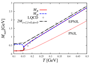
Fig. 2: $T$ dependence of pion and sigma-meson screening masses, $M_{\pi,{\rm scr}}$ and $M_{\sigma,{\rm scr}}$.

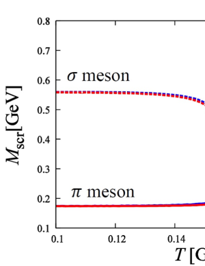
Fig. 3: $T$ dependence of screening and pole mass in pion and sigma-meson.

4 Summary

We have proposed a practical way of calculating meson screening masses $M_{{\xi,\rm scr}}$ in the NJL-type models. This method based on the PV regularization solves the well-known difficulty that the evaluation of $M_{{\xi,\rm scr}}$ is not easy in the NJL-type effective models. In the previous formalism [3], the vacuum and temperature cuts appear in the complex-$\tilde{q}$ plane. The contributions to the mesonic correlation function are partially canceled in the present formalism. The branch point of the resultant cut can be regarded as the threshold mass. The pion and sigma-meson screening masses rapidly approach the threshold mass $2M_{i=1,l=0,\alpha=0}(T)$ after the chiral restoration. We propose the prediction for pole mass from screening mass by using EPNJL model.

- [1] M. Cheng, S. Datta, A. Francis, J. van der Heide, C. Jung, O. Kaczmarek, F. Karsch and E. Laermann et al., Eur. Phys. J. C 71, 1564 (2011).
- [2] T. Kunihiro, Nucl. Phys. B 351, 593 (1991).
- [3] W. Florkowski, Acta. Phys. Pol. B 28, 2079 (1997).
- [4] H. Hansen, W. M. Alberico, A. Beraudo, A. Molinari, M. Nardi, and C. Ratti, Phys. Rev. D 75, 065004 (2007).
- [5] M. Ishii, T. Sasaki, K. Kashiwa, H. Kouno, and M. Yahiro, Phys. Rev. D 89, 071901(R) (2014).
- [6] Y. Sakai, T. Sasaki, H. Kouno, and M. Yahiro, Phys. Rev. D 82, 076003 (2010).
- [7] S. Rößner, C. Ratti, and W. Weise, Phys. Rev. D 75, 034007 (2007).
- [8] W. Pauli, and F. Villars, Rev. Mod. Phys. 21, 434 (1949).
- [9] A. Bazavov et al., Phys. Rev. D 80, 014504 (2009); A. Bazavov et al., Phys. Rev. D 85, 054503 (2012);