Modeling the surface temperature of Earth-like planets

Abstract

We introduce a novel Earth-like planet surface temperature model (ESTM) for habitability studies based on the spatial-temporal distribution of planetary surface temperatures. The ESTM adopts a surface Energy Balance Model complemented by: radiative-convective atmospheric column calculations, a set of physically-based parameterizations of meridional transport, and descriptions of surface and cloud properties more refined than in standard EBMs. The parameterization is valid for rotating terrestrial planets with shallow atmospheres and moderate values of axis obliquity ($\epsilon\lesssim 45^{\circ}$). Comparison with a 3D model of atmospheric dynamics from the literature shows that the equator-to-pole temperature differences predicted by the two models agree within $\approx 5$ K when the rotation rate, insolation, surface pressure and planet radius are varied in the intervals $0.5\lesssim\Omega/\Omega_{\oplus}\lesssim 2$, $0.75\lesssim S/S_{\circ}\lesssim 1.25$, $0.3\lesssim p/(\mathrm{1\,bar})\lesssim 10$, and $0.5\lesssim R/R_{\oplus}\lesssim 2$, respectively. The ESTM has an extremely low computational cost and can be used when the planetary parameters are scarcely known (as for most exoplanets) and/or whenever many runs for different parameter configurations are needed. Model simulations of a test-case exoplanet (Kepler-62e) indicate that an uncertainty in surface pressure within the range expected for terrestrial planets may impact the mean temperature by $\sim 60\,$K. Within the limits of validity of the ESTM, the impact of surface pressure is larger than that predicted by uncertainties in rotation rate, axis obliquity, and ocean fractions. We discuss the possibility of performing a statistical ranking of planetary habitability taking advantage of the flexibility of the ESTM.

1 Introduction

The large amount of exoplanet data collected with the doppler and transit methods (e.g. Mayor et al., 2014; Batalha, 2013, and refs. therein) indicate that Earth-size planets are intrinsically more frequent than giant ones, in spite of the fact that they are more difficult to detect. Small planets are found in a relatively broad range of metallicities (Buchhave et al., 2012) and, at variance with giant planets, their detection rate drops slowly with decreasing metallicity (Wang & Fischer, 2015). These observational results indicate that Earth-like planets are quite common around other stars (e.g. Farr et al., 2014) and are expected to be detected in large numbers in the future. Their potential similarity to the Earth makes them primary targets in the quest for habitable environments ouside the Solar System. Unfortunately, small planets are quite difficult to characterize with experimental methods and a significant effort of modelization is required to cast light on their properties. The aim of the present work is to model the surface temperature of these planets as a contribution to the study of their surface habitability. The capability of an environment to host life depends on many factors, such as the presence of liquid water, nutrients, energy sources, and shielding from cosmic ionizing radiation (e.g. Seager, 2013; Guedel et al., 2014). A knowledge of the surface temperature is essential to apply the liquid water criterion of habitability and can also be used to assess the potential presence of different life forms according to other types of temperature-dependent biological criteria (e.g. Clarke, 2014). Here we are interested in modeling the latitudinal and seasonal variations of surface temperature, $T(\varphi,t)$, as a tool to calculate temperature-dependent indices of fractional habitability (e.g. Spiegel et al., 2008).

Modeling $T(\varphi,t)$ is a difficult task since many of the physical and chemical quantities that govern the exoplanet surface properties are currently not measurable. A way to cope with this problem is to treat the unknown quantities as free parameters and use fast climate calculations to explore how variations of such parameters affect the surface temperature. General Circulation Models (GCMs) are not suited for this type of exploratory work since they require large amounts of computational resources for each single run as well as a detailed knowledge of many planetary characteristics. Two types of fast climate tools are commonly employed in studies of planetary habitability: single atmospheric column calculations and energy balance models. Atmospheric column calculations treat in detail the physics of vertical energy transport, taking into account the influence of atmospheric composition on the radiative transfer (e.g., Kasting, 1988). This is the type of climate tool that is commonly employed in studies of the “habitable zone” (e.g., Kasting, 1988; Kasting et al., 1993; von Paris et al., 2013; Kopparapu et al., 2013, 2014). Energy balance models (EBMs) calculate the zonal and seasonal energy budget of a planet using a heat diffusion formalism to describe the horizontal transport and simple analytical functions of the surface temperature to describe the vertical transport (e.g., North et al., 1981). EBMs have been employed to address the climate impact induced by variations of several planet parameters, such as axis obliquity, rotation period and stellar insolation (Spiegel et al., 2008, 2009; Dressing et al., 2010; Spiegel et al., 2010; Forgan, 2012, 2014). By feeding classic EBMs with multi-parameter functions extracted from atmospheric column calculations one can obtain an upgraded type of EBM that takes into account the physics of vertical transport (Williams & Kasting, 1997). Following a similar approach, in a previous paper we investigated the impact of surface pressure on the habitability of Earth-like planets by incorporating a physical treatment of the thermal radiation and a simple scaling law for the meridional transport (Vladilo et al., 2013, hereafter Paper I). Here we include the transport of the short-wavelength radiation and we present a physically-based treatment of the meridional transport tested with 3D experiments. In this way we build up an Earth-like planet Surface Temperature Model (ESTM) in which a variety of unknown planetary properties can be treated as free parameters for a fast calculation of the surface habitability. The ESTM is presented in the next section. In Section 3 we describe the model calibration and validation. Examples of model applications are presented in Section 4 and the conclusions summarized in Section 5.

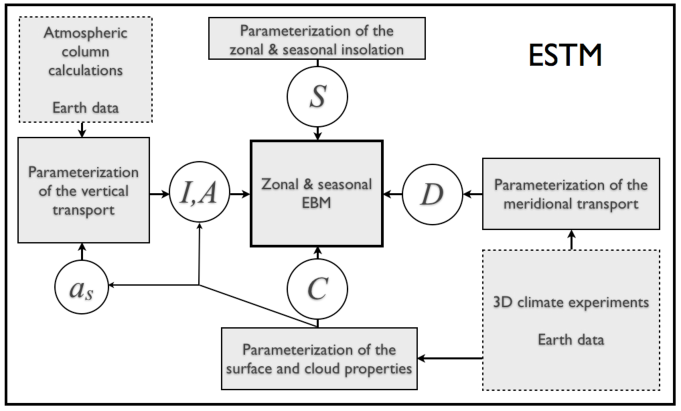
Figure 1: Scheme of the Earth-like planet Surface Temperature Model (ESTM). The zonal and seasonal EBM (central box) is fed by physical quantities (circled symbols) described in §2. At variance with classic EBMs, the physical quantities are multi-parameter functions modelled with the aid of atmospheric column calculations ($I$ and $A$) and 3D climate experiments ($D$).

2 The model

The ESTM consists of a set of climate tools and algorithms that interchange physical quantities expressed in parametric form. The core of the model is a zonal and seasonal EBM fed by multi-parameter physical quantities. The parameterization is obtained using physically-based climate tools that deal with the meridional and vertical energy transport. The relationship between these ingredients is shown in the scheme of Fig. 1. In the following we present the components of the model, starting from the description of the EBM.

In zonal EBMs the surface of the planet is divided into zones delimited by latitude circles. The surface quantities of interest are averaged in each zone over one rotation period. In this way, the spatial dependence is determined by a single coordinate, the latitude $\varphi$. Since the temporal dependence is “smoothed” over one rotation period, the time, $t$, represents the seasonal evolution during the orbital period. The thermal state is described by a single temperature, $T=T(\varphi,t)$, representative of the surface conditions. By assuming that the heating and cooling rates are balanced in each zone, one obtains an energy balance equation that is used to calculate $T(\varphi,t)$. The most common form of EBM equation (North et al., 1981; Williams & Kasting, 1997; Spiegel et al., 2008; Pierrehumbert, 2010; Gilmore, 2014) is

$$C\frac{\partial T}{\partial t}-\frac{\partial}{\partial x}\left[D\,(1-x^{2})\,\frac{\partial T}{\partial x}\right]+I=S\,(1-A),$$ (1)

where $x=\sin\varphi$ and all terms are normalized per unit area. The first term of this equation represents the zonal heat storage and describes the temporal evolution of each zone; $C$ is the zonal heat capacity per unit area (North et al., 1981). The second term represents the amount of heat per unit time and unit area leaving each zone along the meridional direction (North et al., 1981, Eq. (21)). It is called the “diffusion term” because the coefficient $D$ is defined on the basis of the analogy with heat diffusion, i.e.

$$\Phi\equiv-D\frac{\partial T}{\partial\varphi},$$ (2)

where $2\pi R^{2}\Phi\cos\varphi$ is the net rate of energy transport across a circle of constant latitude and $R$ is the planet radius (see Pierrehumbert, 2010). The term $I$ represents the thermal radiation emitted by the zone, also called Outgoing Longwave Radiation (OLR). The right side of the equation represents the fraction of stellar photons that heat the surface of the zone; $S$ is the incoming stellar radiation and $A$ the planetary albedo at the top of the atmosphere. All coefficients of the equation depend, in general, on both time and latitude, either directly or indirectly, through their dependence on $T$.

In classic EBMs the coefficients $D$, $I$ and $A$ are expressed in a very simplified form. As an example, $D$ is often treated as a constant, in spite of the fact that the meridional transport is influenced by planetary quantities that do not appear in the formulation (2). The OLR and albedo are modelled as simple analytical functions, $I=I(T)$ and $A=A(T)$, while they should depend not only on $T$, but also on other physical/chemical quantities that influence the vertical transport. This simplified formulation of $D$, $I$ and $A$ prevents important planetary properties to appear in the energy balance equation (1). To obtain a physically-based parameterization we describe the vertical transport using single-column atmospheric calculations and the meridional transport using algorithms tested with 3D climate experiments. Thanks to this type of parameterization the ESTM features a dependence on surface pressure, $p$, gravitational acceleration, $g$, planet radius, $R$, rotation rate, $\Omega$, surface albedo, $a_{s}$, stellar zenith distance, $Z$, atmospheric chemical composition, and mean radiative properties of the clouds. By running the simulations described in Appendix A, the ESTM generates a “snapshot” of the surface temperature $T(\varphi,t)$ in a very short computing time, for any combination of planetary parameters that yield a stationary solution of Eq. (1). We now describe the parameterization of the model.

2.1 The meridional transport

The heat diffusion analogy (2) guarantees the existence of physical solutions and contributes to the high computational efficiency of EBMs. In order to keep these advantages and at the same time introducing a more realistic treatment of the latitudinal transport, here we derive $\Phi$ and $D$ in terms of planet properties relevant to the physics of the horizontal transport. To keep the problem simple we focus on the atmospheric transport (the ocean transport is discussed below in §2.1.3). The atmospheric flux can be derived applying basic equations of fluid dynamics to the energy content of a parcel of atmospheric gas. The energy budget of the parcel is expressed in terms of the moist static energy (MSE) per unit mass,

$$m=c_{p}T+L_{v}r_{v}+gz$$ (3)

where the terms $c_{p}T$, $L_{v}r_{v}$ and $gz$ measure the sensible heat, the latent heat and the potential energy content of the parcel at height $z$, respectively; $L_{v}$ is the latent heat of the phase transition between the vapor and the condensed phase; $r_{v}$ the mass mixing ratio of the vapor over dry component; $g$ is the surface gravity acceleration. The MSE and the velocity of the parcel are a function of time, $t$, longitude, $\lambda$, latitude, $\varphi$, and height, $z$. The latitudinal transport is obtained by integrating the fluid equations in longitude and vertically, the height $z$ being replaced by the pressure coordinate, $p=p(z)$. Starting from a simplified mass continuity relation valid for the case in which condensation takes away a minimal atmospheric mass (Pierrehumbert, 2010, §9.2.1), one obtains the mean zonal flux

$$\Phi(t,\varphi)=\frac{1}{R}\int_{0}^{2\pi}d\lambda\int_{0}^{p}vm\frac{dp^{\prime}}{g}=\frac{1}{R}\frac{p}{g}\,\overline{v\,m}$$ (4)

where $p$ is the surface atmospheric pressure and $v$ the meridional velocity component of the parcel. The second equality of this expression is valid for a shallow atmosphere, where $g$ can be considered constant, as in the case of the Earth.

To proceed further, we assume that (4) is valid when the physical quantities are averaged over one rotation period, since this is the approach used in EBMs. In this case, the time $t$ represents the seasonal (rather than instantaneous) evolution of the system: variability on time scales shorter than one planetary day are averaged out. At this point we split the problem in two parts. First we derive a relation for $\Phi$ and $D$ valid for the extratropical transport regime. Then we introduce a formalism to empirically improve the treatment of the transport inside the Hadley cells.

2.1.1 Transport in the extratropical region

We consider an ideal planet with constant insolation and null axis obliquity, in such a way that we can neglect the (seasonal) dependence on $t$. We restrict our problem to the atmospheric circulation typical of fast-rotating terrestrial-type planets, i.e. with latitudinal transport dominated by eddies in the baroclinic zone. A commonly adopted formalism used to treat the eddies consists in dividing the variables of interest into a mean component and a perturbation from the mean , representative of the eddies. By indicating the mean with an overbar and perturbations with a prime, we have for instance $v=\overline{v}+v^{\prime}$ and $m=\overline{m}+m^{\prime}$. It is easy to show that $\overline{vm}=\overline{v}\,\overline{m}+\overline{v^{\prime}m^{\prime}}$. When the eddies transport dominates, the term $\overline{v}\,\overline{m}$ can be neglected so that

$$\Phi\simeq\frac{1}{R}\frac{p}{g}\,\overline{v^{\prime}m^{\prime}}$$ (5)

and we obtain

$$D=-\Phi\left(\frac{\partial T}{\partial\varphi}\right)^{-1}=\frac{1}{R^{2}}\frac{p}{g}\,\left(\frac{\partial T}{\partial y}\right)^{-1}\,\overline{v^{\prime}m^{\prime}}$$ (6)

where $dy=R\,d\varphi$ is the infinitesimal meridional displacement. To calculate $\overline{v^{\prime}m^{\prime}}$ we consider the surface value of moist static energy, $m=c_{p}T+L_{v}r_{v}$, from which we obtain

$$\overline{v^{\prime}m^{\prime}}=c_{p}\overline{v^{\prime}T^{\prime}}+L_{v}\overline{v^{\prime}r^{\prime}_{v}}~{}.$$ (7)

We express the mean values of the perturbation products as

$$\overline{v^{\prime}T^{\prime}}=k_{\mathrm{S}}\,|v^{\prime}|~{}|T^{\prime}|$$ (8)

and

$$\overline{v^{\prime}r_{v}^{\prime}}=k_{\mathrm{L}}|v^{\prime}|~{}|r_{v}^{\prime}|,$$ (9)

where $||$ means a root-mean square magnitude and $k_{\mathrm{S}}$ and $k_{\mathrm{L}}$ are correlation coefficients (e.g. Barry et al., 2002). At this point we need to quantify the perturbations of $T$ and $r_{v}$, i.e. of the quantities being mixed. In eddy diffusivity theories these perturbations can be written as a mixing length, $\ell_{\mathrm{mix}}$, times the spatial gradient of the quantity. We consider the gradient along the meridional coordinate $y$ and we write

$$|T^{\prime}|=-\ell_{\mathrm{mix}}\frac{\partial T}{\partial y}$$ (10)

and

$$|r_{v}^{\prime}|=-\ell_{\mathrm{mix}}\frac{\partial\,r_{v}}{\partial y}$$ (11)

where $T$ and $r_{v}$ are mean zonal quantities; since the mixing is driven by turbulence we assume that the mixing length is the same for sensitive and latent heat. To estimate $\partial r_{v}/\partial y$ we recall that

$$r_{v}=\frac{\mu_{v}}{\mu_{\mathrm{dry}}}\frac{p_{v}}{p_{\mathrm{dry}}}=\frac{\mu_{v}}{\mu_{\mathrm{dry}}}\frac{q\,p_{v}^{*}}{p_{\mathrm{dry}}}$$ (12)

where $\mu_{v}$ and $p_{v}$ are the molecular weight and pressure of the vapor, $\mu_{\text{dry}}$ and $p_{\text{dry}}$ the corresponding quantities of the dry air, $q$ is the relative humidity and $p_{v}^{*}=p_{v}^{*}(T)$ is the saturation vapor pressure. We assume constant relative humidity and we can write

$$\frac{\partial r_{v}}{\partial y}=\left(\frac{\partial\,r_{v}}{\partial T}\cdot\frac{\partial T}{\partial y}\right)=\frac{\mu_{v}}{\mu_{\mathrm{dry}}}\frac{q}{p_{\mathrm{dry}}}\frac{\partial p_{v}^{*}}{\partial T}\,\frac{\partial T}{\partial y}~{}.$$ (13)

Combining the expressions from (7) to (13) we obtain

$$\overline{v^{\prime}m^{\prime}}=-\ell_{\mathrm{mix}}\,|v^{\prime}|\,\frac{\partial T}{\partial y}\left(k_{\mathrm{S}}c_{p}+k_{\mathrm{L}}L_{v}\frac{\mu_{v}}{\mu_{\mathrm{dry}}}\frac{q}{p_{\mathrm{dry}}}\frac{\partial p_{v}^{*}}{\partial T}\right)$$ (14)

and inserting this in (6) we derive

$$D\simeq\frac{1}{R^{2}}\frac{p}{g}\ell_{\mathrm{mix}}\,|v^{\prime}|\,\left(k_{\mathrm{S}}c_{p}+k_{\mathrm{L}}L_{v}\frac{\mu_{v}}{\mu_{\mathrm{dry}}}\frac{q}{p_{\mathrm{dry}}}\frac{\partial p_{v}^{*}}{\partial T}\right)~{}.$$ (15)

At this point, we need an analytical expression for $\ell_{\mathrm{mix}}\,|v^{\prime}|$. Among a large number of analytical treatments of the baroclinic circulation (e.g., Green, 1970; Stone, 1972; Gierasch & Toon, 1973; Held, 1999), here we adopt a formalism proposed by Barry et al. (2002) which gives the best agreement with GCM experiments.

According to Barry et al. (2002), the baroclinic zone works as a diabatic heat engine that obtains and dissipates energy in the process of transporting heat from a warm to a cold region. If we call $T_{w}$ and $T_{c}$ the temperatures of the warm and cold regions, the maximum possible thermodynamic efficiency of the engine is $\delta T/T_{w}$, where $\delta T=T_{w}-T_{c}$. The energy received by the atmosphere per unit time and unit mass, $Q$, represents the diabatic forcing of the engine. The rate of generation (and dissipation) of eddy kinetic energy per unit mass is given by

$$\varepsilon=\eta\,\left(\frac{\delta T}{T_{w}}\right)\,Q$$ (16)

where $\eta$ is an efficiency factor representing the fraction of the generated kinetic energy used by heat transporting eddies. Assuming that the average properties of the flow depend only on the length scale and the dissipation rate per unit mass, dimensional arguments yield the velocity scaling law

$$|v^{\prime}|\propto\left(\varepsilon\,\ell_{\mathrm{mix}}\right)^{1/3}~{}.$$ (17)

As far as the mixing length is concerned, the Rhines scale is adopted

$$\ell_{\mathrm{mix}}=\left(\frac{2|v^{\prime}|}{\beta}\right)^{1/2}$$ (18)

where $\beta=\partial f/\partial y$ is the gradient of the Coriolis parameter, $f=2\Omega\sin\varphi$, and $\Omega$ the angular rotation rate of the planet. The study of Barry et al. (2002) suggests that, among other types of length scales considered in literature, the Rhines scale yields the best correlations in 3D atmospheric experiments. The adoption of the Rhines scale is also supported by a study of moist transport performed with GCM experiments (Frierson et al., 2007). The Rhines scale must be calculated at the latitude $\varphi_{\mathrm{m}}$ of maximum kinetic energy, i.e. for $\beta=(2\Omega\cos\varphi_{\mathrm{m}})/R$. From the above expressions we obtain

$$\ell_{\mathrm{mix}}\,|v^{\prime}|=\left(\eta\frac{\delta T}{T_{w}}\,Q\right)^{3/5}\left(\frac{R}{\Omega\cos\varphi_{\mathrm{m}}}\right)^{4/5}~{}.$$ (19)

Inserting this in (15) we obtain

$$D=D_{\mathrm{dry}}(1+\Lambda)$$ (20)

where

$$D_{\mathrm{dry}}=k_{\mathrm{S}}c_{p}\,\eta^{3/5}(\cos\varphi_{\mathrm{m}})^{-4/5}\times$$ (21)

$${}\times\,R^{-6/5}\,\frac{p}{g}\,\Omega^{-4/5}\left(\frac{\delta T}{T_{w}}Q\right)^{3/5}$$

is the dry component of the atmospheric eddies transport and

$$\Lambda=\frac{k_{\mathrm{L}}L_{v}}{k_{\mathrm{S}}c_{p}}\frac{\mu_{v}}{\mu_{\mathrm{dry}}}\frac{q}{p_{\mathrm{dry}}}\frac{\partial p_{v}^{*}}{\partial T}$$ (22)

is the ratio of the moist over dry components.

For the practical implementation of the analytical expressions (20), (21) and (22) in the EBM code, we proceed as follows. The maximum thermodynamic efficiency $\delta T/T_{w}$ is calculated by taking $T_{w}=\overline{T}(\varphi_{1})$ and $T_{c}=\overline{T}(\varphi_{2})$ where $\varphi_{1}$ and $\varphi_{2}$ are the borders of the mid-latitude region and overbars indicate zonal annual means. Following Barry et al. (2002), we adopt $\varphi_{1}=28^{\circ}$ and $\varphi_{2}=68^{\circ}$, after testing that the model predictions are virtually unaffected by the exact choice of these values. We estimate the diabatic forcing term (W/kg) as $Q\simeq\left\{\mathrm{ASR}\right\}/(p/g)$, where $\left\{\mathrm{ASR}\right\}=\left\{S(1-A)\right\}$ is the absorbed stellar radiation (W/m²) averaged over one orbital period in the latitude range ($\varphi_{1}$, $\varphi_{2}$) and $p/g$ the atmospheric columnar mass (kg/m²). We neglect the contribution of surface fluxes of sensible heat since they cannot be estimated in the framework of the EBM model. This approximation is not critical because these fluxes yield a negligible contribution to $Q$ according to Barry et al. (2002). Treating $k_{\mathrm{L}}$, $k_{\mathrm{S}}$, $\eta$, and $\varphi_{\mathrm{m}}$ as constants, we obtain from Eq. (21) a scaling law for the dry term of the transport

$$\mathcal{S}_{\mathrm{dry}}\propto c_{p}\,R^{-6/5}\left(\frac{p}{g}\right)^{2/5}\Omega^{-4/5}\times{}$$ (23)

$${}\times\left(\frac{\delta T}{T_{w}}\left\{\mathrm{ASR}\right\}\right)^{3/5}.$$

We estimate the temperature gradient of saturated vapor pressure as $\partial p_{v}^{*}/\partial T\simeq\delta p_{v}^{*}/\delta T$, with $\delta p_{v}^{*}=\left[p_{v}^{*}(T_{w})-p_{v}^{*}(T_{c})\right]$. Since $k_{\mathrm{L}}$, $k_{\mathrm{S}}$ and $L_{v}$ are constants, we obtain from Eq. (22) a scaling law for the ratio of the moist over dry components

$$\mathcal{S}_{\mathrm{md}}\propto\frac{q}{c_{p}\,\mu_{\mathrm{dry}}\,p_{\mathrm{dry}}}\frac{\delta p_{v}^{*}}{\delta T}~{}.$$ (24)

Finally, by applying Eq. (20) and the scaling laws (23) and (24) to a generic terrestrial planet and to the Earth, indicated by the subscript $\circ$, we obtain

$$\frac{D}{D_{\circ}}=\frac{\mathcal{S}_{\mathrm{dry}}}{\mathcal{S}_{\mathrm{dry},\circ}}\,\left[\frac{1+\Lambda_{\circ}\cdot\left(\mathcal{S}_{\mathrm{md}}/\mathcal{S}_{\mathrm{md},\circ}\right)}{1+\Lambda_{\circ}}\right]~{}.$$ (25)

With the above expressions we calculate $D$ treating $R$, $\Omega$, $p$, $g$, $c_{p}$, $\mu_{\mathrm{dry}}$, $p_{\mathrm{dry}}$, $q$ as parameters that can vary from planet to planet, in spite of being constant in each planet. The ratio of moist over dry eddie transport of the Earth is set to $\Lambda_{\circ}=0.7$ (e.g. Kaspi & Showman, 2014). For the sake of self-consistency, we adopt the parameters $(\delta_{T})_{\circ}$, $(T_{w})_{\circ}$, $\left\{\mathrm{ASR}\right\}_{\circ}$ and $(\delta p_{v}^{*})_{\circ}$ obtained from the Earth’s reference model. Since these parameters vary in the course of the simulation, we perform the calibration of the Earth model in two steps. First we calibrate the model excluding the ratios $\delta_{T}/(\delta_{T})_{\circ}$, $T_{w}/T_{w,\circ}$, $\left\{\mathrm{ASR}\right\}/\left\{\mathrm{ASR}\right\}_{\circ}$ and $\delta p_{v}^{*}/(\delta p_{v}^{*})_{\circ}$ from the scaling laws of Eq. (25). Then we reintroduce these ratios in the scaling law adopting for $(\delta_{T})_{\circ}$, $(T_{w})_{\circ}$ and $\left\{\mathrm{ASR}\right\}_{\circ}$ the values $(\delta_{T})$, $(T_{w})$, $\left\{\mathrm{ASR}\right\}$ and $(\delta p_{v}^{*})$ obtained in the first step. The second step is repeated a few times, until convergence of the parameters $(\delta_{T})_{\circ}$, $(T_{w})_{\circ}$ and $\left\{\mathrm{ASR}\right\}_{\circ}$ and $(\delta p_{v}^{*})_{\circ}$ is achieved.

2.1.2 Transport in the Hadley Cell

The derivation performed above ignores the existence of the Hadley Cells, since they do not contribute to the extratropical meridional transport. However, the Hadley circulation is extremely efficient in smoothing temperature gradients inside the tropical region. This aspect cannot be completeley ignored in our treatment, since our goal is to estimate the planet surface temperature distribution. Unfortunately, the diffusion formalism of Eq. (2) is inappropriate inside the Hadley Cells and the only way we have to improve the description of the tropical temperature distribution is to correct the formalism with some empirical expression. We summarize the approach that we follow to cope with this problem.

The global pattern of atmospheric circulation is influenced, among other factors, by the seasonal variation of the zenith distance of the star. In the case of the Earth, a well known example of this type of influence is the seasonal shift of the Intertropical Convergence Zone (ITCZ), that moves to higher latitudes in the summer hemisphere. The ITCZ is, in practice, a tracer of the thermal equator at the center of the system of the two Hadley Cells, where we want to improve the uniformity of the temperature distribution. A way to do this is to enhance the transport coefficient $D$ in correspondence with such thermal equator. To incorporate this feature in our model, we scale $D$ according to mean diurnal value of $\mu(\varphi,t)=\cos Z$, where $Z$ is the stellar zenith distance. In practice, we multiply $D$ by a dimensionless modulating factor, $\zeta(\varphi,t)$, that scales linearly with $\mu(\varphi,t)$, i.e. $\zeta(\varphi,t)=c_{o}+c_{1}\mu(\varphi,t)$. We normalize this factor in such a way that its mean global annual value is $\widetilde{\zeta}(\varphi,t)=1$. Thanks to the normalization condition, it is possible to calculate the parameters $c_{0}$ and $c_{1}$ in terms of a single parameter, $\mathcal{R}=\max\left\{\zeta(\varphi,t)\right\}/\min\left\{\zeta(\varphi,t)\right\}$, which represents the ratio between the maximum and minimum values of $\zeta$ at any latitude and orbital phase (see Vladilo et al., 2013, §A.2.1). With the adoption of the modulation term, the complete expression for the transport coefficient becomes

$$\frac{D}{D_{\circ}}=\zeta(\varphi,t)\,\frac{\mathcal{S}_{\mathrm{dry}}}{\mathcal{S}_{\mathrm{dry},\circ}}\,\left[\frac{1+\Lambda_{\circ}\cdot\left(\mathcal{S}_{\mathrm{md}}/\mathcal{S}_{\mathrm{md},\circ}\right)}{1+\Lambda_{\circ}}\right].$$ (26)

The mean global annual value of this expression equals Eq. (25) thanks to the normalization condition $\widetilde{\zeta}(\varphi,t)=1$. This formalism introduces a dependence on $t$ and on the axis obliquity in the transport coefficient.

Empirical support for the adoption of the modulation term $\zeta(\varphi,t)$ comes from the improved match between the observed and predicted temperature-latitude profile of the Earth. In the left panel of Fig. 2 we show that it is not possible to accurately match the Earth profile by varying $D_{\circ}$ at constant $\zeta(\varphi,t)=1$ (i.e. $\mathcal{R}=1$). This is because the whole profile becomes flatter with increasing $D_{\circ}$ and the values of $D_{\circ}$ sufficiently high to provide the desired smooth temperature distribution inside the tropics yield a profile which is too flat in the polar regions. This problem can be solved with the introduction of the modulation factor $\zeta$. In the right panel of Fig. 2 we show that by increasing $\mathcal{R}$ the profile declines faster at the poles while becoming slightly flatter at the equator. This behavior is different from that induced by changes of $D_{\circ}$ and provides an extra degree of freedom to match the observed profile. For the time being, the parameter $\mathcal{R}$ can be tuned to fit the Earth model, but cannot be validated with other planets. The validation of $\mathcal{R}$ in rocky planets different from the Earth could be addressed by future GCM calculations. Meantime, the uncertainty related to the choice of this parameter in other planets can be estimated by repeating the climate simulations for different values of $\mathcal{R}$. Given the lack of solid theoretical support for the adoption of the $\zeta(\varphi,t)$ formalism, it is safe to use the smallest possible value of $\mathcal{R}$ (i.e. closest to unity) that allows the Earth profile to be reproduced. With the upgraded calibration of the Earth model presented here (Appendix B) we have been able to adopt a lower value ($\mathcal{R}=2.2$, Table 1) than in Paper I ($\mathcal{R}=6$, Table 2 in Vladilo et al. (2013)).

2.1.3 Ocean transport

The algorithm that describes the energy transport has been derived assuming that most of the meridional transport is performed by the atmosphere rather than the ocean (§2.1). This is a reasonable assumption in the Earth climate regime, where the atmosphere contributes 78% of the total transport in the Northern Hemisphere and 92% in the Southern Hemisphere at the latitude of maximum poleward transport (Trenberth & Caron, 2001). In order to assess the importance of the ocean contribution in different planetary regimes one needs to run GCM simulations featuring the ocean component. This is a difficult task because the ocean circulation is extremely dependent on the detailed distribution of the continents and because the time scale of ocean response is much longer than that of the atmosphere. As a result, one should run GCMs with a detailed description of the geography for a large number of orbits in order to include the ocean transport in the modellization of exoplanets. With this type of climate simulation it would be impossible to perform an exploratory study of exoplanet surface temperature, which is the aim of our model. Not to mention the fact that the choice of a detailed description of the continental distribution in exoplanets is completely arbitrary. It is therefore desirable to find simplified algorithms able to include the ocean transport in zonal models, such as the ESTM. To this end, one should perform 3D numerical experiments aimed at investigating how the energy transport is partitioned between the atmosphere and the ocean in a variety of planetary conditions. Preliminary work of this type suggests that the energy transport of wind-driven ocean gyres vary in a roughly similar fashion to the energy transport of the atmosphere as external parameters vary (Vallis & Farneti, 2009). The existence of mechanisms of compensation that regulate the relative contribution of the atmosphere and the ocean to the total transport (Bjerknes, 1964; Shaffrey & Sutton, 2006; van der Swaluw et al., 2007; Lucarini & Ragone, 2011) may also help build a simplified description of the atmosphere/ocean transport. In the case of the Earth, we note that the total transport is remarkably similar in the Southern and Northern hemisphere (see Fig. 7) in spite of significant differences between the two hemispheres in terms of the relative contribution of the ocean and atmosphere (e.g. Trenberth & Caron, 2001, Fig. 7).

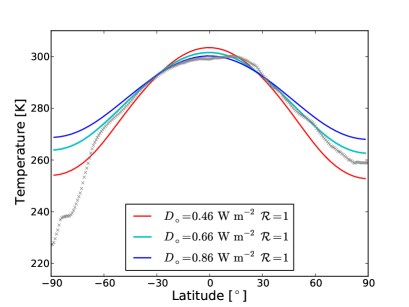
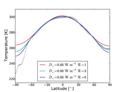
Figure 2: Annual temperature-latitude profile of the Earth model obtained by varying the transport parameters $D_{\circ}$ and $\mathcal{R}$. Left panel: variation of $D_{\circ}$ at $\mathcal{R}=1$ (i.e. without seasonal modulation of the transport coefficient). Right panel: variation of the strength of seasonal modulation, $\mathcal{R}$, at constant $D_{\circ}$. See §2.1.2.

2.2 The vertical transport

The outgoing longwave radiation and the top-of-atmosphere albedo are parametrized using single atmospheric column calculations. In the present version of the ESTM, the single column calculations are performed with standard radiation codes developed at the National Center for Atmospheric Research (NCAR), as part of the Community Climate Model (CCM) project NCAR-CCM (Kiehl et al., 1998). To access these codes we use the set of routines CliMT (Pierrehumbert, 2010; Caballero, 2012).

The CCM code employs an Earth-like atmospheric composition, with the possibility to change the amount of non-condensable greenhouse gases (i.e. CO₂ and CH₄). We adopt $p\mathrm{CO}_{2}=380$ ppmv and $p\mathrm{CH}_{4}=1.8$ ppmv as the reference values for the Earth’s model. These values can be changed as long as they remain in trace abundances, as in the case of the Earth. The relative humidity, $q$, is fixed to limit the huge amount of calculations and the dimensions of the tables described below. We adopt $q=0.6$, a value consistent with the global relative humidity measured on Earth. A low effective humidity ($q\sim 0.6$) is predicted self-consistently by 3-D dynamic climate models as a result of subsidence in the Hadley circulation (e.g. Ishiwatari et al., 2002). Adoption of saturated water vapour pressure ($q=1$) tends to understimate the OLR at high temperatures, leading to excessive heating of the planet.

2.2.1 Outgoing long-wavelength radiation

We use a column radiation model scheme for a cloud-free atmosphere to calculate the Outgoing Long-wavelength Radiation (OLR), i.e. the thermal infrared emission that cools the planet. The OLR calculations are repeated a large number of times in order to cover a broad interval of surface temperature, $T$, background pressure, $p$, gravity acceleration, $g$, and partial pressure of non-condensable greenhouse gases. The results of these calculations are stored in tables OLR=OLR$(T,p,g,p\mathrm{CO}_{2},p\mathrm{CH}_{4})$. In the course of the simulation, these tables are interpolated at the zonal and instantaneous value of $T=T(\varphi,t)$. The long-wavelength forcing of the clouds is subtracted at this stage, taking into account the zonal cloud coverage, as we explain in §2.3.2. The total CPU time required to cover the parameter space $(T,p,g,p\mathrm{CO}_{2},p\mathrm{CH}_{4})$ is relatively large. However, once the tables are built up, the simulations are extremely fast.

2.2.2 Incoming short-wavelength radiation

The top-of-atmosphere albedo, $A$, is calculated with the CCM code, to take into account the transfer of short-wavelength stellar photons in the planet atmosphere. In each atmospheric column we calculate the fraction of stellar photons that is reflected back in space for different values of $T$, $p$, $g$, $p\mathrm{CO_{2}}$, surface albedo, $a_{s}$, and zenith distance of the star, $Z$. In practice, for each set of values ($g$, $p\mathrm{CO}_{2}$, $p\mathrm{CH}_{4}$), we calculate the temperature and pressure dependence of $A$. Then, for each set of values $(T,p,g,p\mathrm{CO_{2}},p\mathrm{CH}_{4})$ the calculations are repeated to cover the complete intervals of surface albedo, $0<a_{\mathrm{s}}<1$, and zenith distance, $0^{\circ}<Z<90^{\circ}$. The results of these calculations are stored in multidimensional tables. In the course of the ESTM simulations these tables are interpolated to calculate $A$ as a function of the zonal and instantaneous values of $(T,p,g,p\mathrm{CO_{2}},a_{\mathrm{s}},Z)$. Each single column calculation of $A$ is relatively fast, compared to the corresponding calculation of $I$. However, due to the necessity of covering a larger parameter space, the preparation of the tables $A=A(T,p,g,p\mathrm{CO_{2}},a_{\mathrm{s}},Z)$ requires a comparable CPU time.

2.2.3 Caveats

The CCM calculations that we use include pressure broadening (Kiehl et al., 1998, and refs. therein), but not collision-induced absorption. As a result, the model may underestimate the atmospheric absorption at the highest values of pressure. To avoid physical conditions not considered in the calculations we limit the surface pressure at $p\lesssim 10$ bar.

The calculations are valid for a solar-type spectral distribution. The spectral type of the central star affects the vertical transport because of the wavelength dependence of the atmospheric albedo (e.g., Selsis et al., 2007). The present version of the ESTM should be applied to planets orbiting stars with spectral distributions not very different from the solar one.

2.3 Surface and cloud properties

2.3.1 Zonal coverage of oceans, lands, ice and clouds

The zonal coverage of oceans is a free parameter, $f_{o}$, that also determines the fraction of continents, $f_{l}=1-f_{o}$. In this way, the planet geography is specified in a schematic way by assigning a set of $f_{o}$ values, one for each zone. The zonal coverage of ice and clouds is parametrized using algorithms calibrated with Earth experimental data. Following WK97, the zonal coverage of ice is a function of the mean diurnal temperature,

$$f_{i}(T)=\max\left\{0,\left[1-e^{(T-273.15\,\mathrm{K})/10\,\mathrm{K}}\right]\right\}.$$ (27)

One problem with this formulation is that the ice melts completely and instantaneously as soon as $T>273.15$ K. To minimize this effect, we introduced an algorithm that mimics the formation of permanent ice when a latitude zone is below the freezing point for more than half the orbital period. In this case, we adopt a constant ice coverage for the full orbit, $f_{i}=f_{i}(\overline{T})$, where $\overline{T}$ is the mean annual zonal temperature.

As far as the clouds are concerned, we adopt specific values of zonal coverage for clouds over oceans and continents. The dependence of the cloud coverage on the type of underlying surface has long been known (e.g. Kondrat ev, 1969) and has been quantified in recent studies (e.g. Sanromá & Pallé, 2012; Stubenrauch, 2013). Based on the results obtained by Sanromá & Pallé (2012), we adopt $0.70$ and $0.60$ for the cloud coverage over oceans and lands, respectively. In this way, the reference Earth model (Appendix B) predicts a mean annual global cloud coverage ${\textstyle<}f_{c,\circ}{\textstyle>}=0.67$, in excellent agreement with most recent Earth data (Stubenrauch, 2013). With our formalism the cloud coverage is automatically adjusted for planets with cloud properties similar to those of the Earth, but different fractions of continents and oceans. Since the coverage of ice, $f_{i}$, depends on the temperature, the model simulates the feedback between temperature and albedo.

2.3.2 Cloud radiative properties

The albedo and infrared absorption of the clouds have cooling and warming effects of the planet surface, respectively. Even with specifically designed 3D models it is hard to predict which of these two opposite effects dominate. The single-column radiative calculations used in studies of habitability usually assume cloud-free radiative transfer and tune the results by playing with the albedo (Kasting, 1988; Kasting et al., 1993; Kopparapu et al., 2013, 2014). The approach that we adopt with the ESTM is to parametrize the albedo and the long-wavelength forcing of the clouds assuming that their global properties are similar to those measured in the present-day Earth. Following WK97, we express the albedo of the clouds as

$$a_{c}=\alpha+\beta Z$$ (28)

where the parameters $\alpha$ and $\beta$ are tuned to fit Earth experimental data of cloud albedo as a function of stellar zenith distance (Cess, 1976). For clouds over ice, we adopt the same albedo of frozen surfaces (see Table 1). To take into account the long wavelength forcing of the clouds, we subtract ${\textstyle<}\mathrm{OLR}{\textstyle>}_{\mathrm{cl,\circ}}\,(f_{c}/{\textstyle<}f_{c,\circ}{\textstyle>})$ from the clear-sky OLR obtained from the radiative calculations, where ${\textstyle<}\mathrm{OLR}{\textstyle>}_{\mathrm{cl,\circ}}=26.4$ W m^-2 is the mean global long wavelength forcing of the clouds on Earth (Stephens et al., 2012), $f_{c}$ is the mean cloud coverage in each latitude zone, and ${\textstyle<}f_{c,\circ}{\textstyle>}=0.67$ the mean global cloud coverage of the reference Earth model.

The fact that the ESTM accounts for the mean radiative properties of the clouds is an improvement over classic EBMs, but one should be aware that the adopted parameterization is only valid for planets with global cloud properties similar to those of the Earth. This is a critical point because the cloud radiative properties may change with planetary conditions, as suggested by 3D simulations of terrestrial planets (e.g. Leconte et al., 2013; Yang et al., 2013). To some extent, we can simulate this situation by changing the ESTM  cloud-forcing parameters. An example of this exercise is provided in Fig. 15. If the predictions of 3D experiments become more robust, it could be possible in the future to introduce a new ESTM recipe for expressing the cloud forcing as a function of relevant planetary parameters.

2.3.3 The surface albedo

The mean surface albedo of each latitude zone is calculated by averaging the albedo of each type of surface present in the zone, weighted according to its zonal coverage. For the surface albedo of continents and ice we adopt the fiducial values listed in Table 1. The albedo of the oceans is calculated as a function of the stellar zenith distance, $Z$, using an expression calibrated with experimental data (Briegleb et al., 1986; Enomoto, 2007)

$$a_{o}={0.026\over(1.1\,\mu^{1.7}+0.065)}+{}$$ (29)

$${}+0.15(\mu-0.1)\,(\mu-0.5)\,(\mu-1.0)~{},$$

where $\mu=\cos Z$. Also clouds are treated as surface features, with zonal coverage and albedo parametrized as explained above (§2.3.2).

2.3.4 Thermal capacity of the surface

The term $C$ is calculated by averaging the thermal capacity per unit area of each type of surface present in the corresponding zone according to its zonal coverage (§2.3.1). The parameters used in these calculations are representative of the thermal capacities of oceans and solid surface (Table 1). For the reference Earth model the ocean contribution is calculated assuming a 50 m, wind-mixed ocean layer (Williams & Kasting, 1997; Pierrehumbert, 2010). The atmospheric contribution is calculated as

$$\left(\frac{C_{\mathrm{atm}}}{C_{\mathrm{atm},\circ}}\right)=\left(\frac{c_{p}}{c_{p,\circ}}\right)\,\left(\frac{p}{p_{\circ}}\right)\,\left(\frac{g_{\circ}}{g}\right)~{}~{}~{},$$ (30)

where $c_{p}$ and $p$ are the specific heat capacity and total pressure of the atmosphere, respectively (Pierrehumbert, 2010). The atmospheric term enters as an additive contribution to the ocean and solid surface terms. Its impact on these parameters is generally small, the ocean contribution being the dominant one.

The strong thermal inertia of the oceans implies that the mean zonal $C$ has an “ocean-like” value even when the zonal fraction of lands is comparable to that of the oceans (Williams & Kasting, 1997). This weak point of the longitudinally-averaged model can be by-passed by adopting an idealized orography with continents covering all longitudes (see §C.6).

2.4 The insolation term $S$

The zonal, instantaneous stellar radiation $S=S(\varphi,t)$ is calculated from the stellar luminosity, the keplerian orbital parameters and the inclination of the planet rotation axis. The model calculates $S$ also for eccentric orbits. Details on the implementation of $S$ can be found in Paper I (Vladilo et al., 2013, §A.5). At variance with that paper, the ESTM takes also into account the vertical transport of short-wavelength photons (see §2.2.2).

2.5 Limitations of the model

In spite of the above-mentioned improvements over classic EBMs, the adoption of the zonal energy balance formalism at the core of the ESTM leads to well known limitations intrinsic to EBMs. One is that zonally averaged models cannot be applied to tidally-locked planets that always expose the same side to their central star: such cases require specifically designed models (e.g., Kite et al., 2011; Menou, 2013; Mills & Abbot, 2013; Yang et al., 2013). Also, it should be clear that the ESTM does not track climatic effects that develop in the vertical direction, even though the atmospheric response is adjusted according to latitudinal and seasonal variations of $T$ and $Z$. In spite of these limitations, the EBM at the core of our climate tools provides the flexibility that is required when many runs are needed or when one wants to compare the impact of different parameters unconstrained by the observations. At present time this is still unfeasible with GCMs and even with Intermediate Complexity Models. While GCMs are invaluable tools for climate change studies on Earth, they are heavily parameterized on current Earth conditions, and their use in significantly different conditions raises concern. In particular, the paper by Stevens & Bony (2013) caused serious worries about the use of GCMs in “unconstrained” situations such as those encountered in habitability studies.

3 Model calibration and validation

The ESTM is implemented in two stages. First, a reference Earth model is built up by tuning the parameters to match the present Earth climate properties (see Appendix B). Then we use results obtained from 3D climate experiments to tune parameters or validate algorithms that are meant to be applied in Earth-like planets. Here we present a test of validation of the algorithms that describe the meridional transport. This test is a concrete example of how results obtained by GCMs can be used to validate the model.

3.1 Validation of the meridional transport

To perform this test we used a study of the atmospheric dynamics of terrestrial exoplanets performed by Kaspi & Showman (2014). These authors employed a moist atmospheric general circulation model to test the response of the atmospheric dynamics over a wide range of planet parameters. Specifically, they used an idealized aquaplanet with surface covered by a uniform slab of water 1 m thick; only vapor-liquid phase change was considered; the albedo was fixed at 0.35 and insolation was imposed equally between hemispheres; the remaining parameters were set to mimic an Earth-like climate. To validate the ESTM with the results found by Kaspi & Showman (2014) we modified the Earth reference model as follows. The axis obliquity was set to zero; the temperature-ice feedback was excluded; the albedo was fixed at $A=0.35$; the fraction of oceans was set to 1, adopting a thermal capacity corresponding to a mixing layer 1 m thick. With this idealized planet model we performed several sets of simulations, varying the planet rotation rate, surface flux, radius, and surface pressure. To validate the ESTM we analyze the mean annual equator-to-pole temperature difference, $\Delta T_{\text{EP}}$, which is critical for a correct estimate of the latitude temperature profile and of the surface habitability. The results of the tests are shown in Fig. 3, where we compare the $\Delta T_{\text{EP}}$ values predicted by the 3D model (diamonds) with those obtained from the ESTM (solid lines). We also plot the predictions of a “dry” transport model (dashed lines) obtained by setting $\Lambda=0$ in Eq. (20). Finally, for the sake of comparison with previous EBMs, we plot the results obtained from a “basic ESTM” without moist term ($\Lambda=0$) and without diabatic forcing term (dotted lines). In using this “basic” model, we test some alternative scaling laws for the parameterization of the rotation rate, surface pressure and radius, as we explain below.

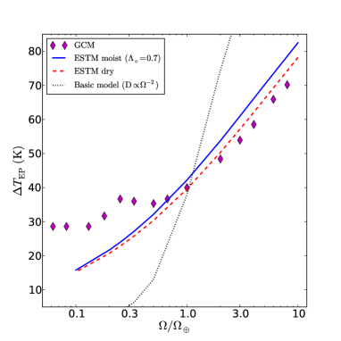
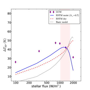
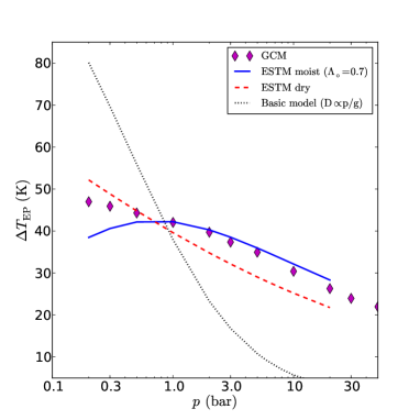
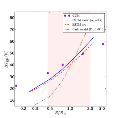
Figure 3: Predicted values of equator-to-pole temperature difference, $\Delta T_{\mathrm{EP}}$, versus planet rotation rate (top left), stellar flux (top right), surface atmospheric pressure (bottom left), and planet radius (bottom right) obtained from different climate simulations of an Earth-like aquaplanet with axis obliquity $\epsilon=0^{\circ}$, fixed albedo ($A=0.35$), and no ice. Magenta diamonds: 3D GCM simulations (Kaspi & Showman, 2014). Solid and dashed curves: ESTM (moist and dry transport, respectively). Dotted curves: ESTM dry model without diabatic forcing term and with different prescriptions for $D$ (see legend in each panel and §3.1.) The shaded area in the top right panel brackets a range of $\pm 25$% the present-day value of Earth’s insolation. The shaded area in the bottom right panel brackets the range of masses 0.1 to 8 M_⊕ for rocky planets with mean density $\rho=\rho_{\oplus}$.

3.1.1 Rotation rate

In this experiment all parameters were fixed, with the exception of the planet rotation rate, $\Omega$, that was gradually increased from 1/10 to 10 times the Earth value, $\Omega_{\oplus}$. The results of this test are shown in the top-left panel of Fig. 3. One can see that the ESTM and GCM results show a similar trend, with a good quantitative agreement at $\Omega\gtrsim 0.3\,\Omega_{\oplus}$, but not at low rotation rate. This result is expected since our parameterization is appropriate to simulate planets with horizontal transport dominated by mid-latitude eddies, i.e. planets with relatively high rotation rate (see §2.1). The dotted line in this figure shows the results of the basic model obtained by replacing the term $\Omega^{-4/5}$ in Eq. (23) with the stronger dependence $\Omega^{-2}$ adopted in previous work (e.g. Williams & Kasting, 1997; Vladilo et al., 2013). One can see that this strong dependence on rotation rate is not supported by the 3D model, while the more moderate dependence $D\propto\Omega^{-4/5}$ adopted in the ESTM yields a much better agreement with the GCM experiments.

3.1.2 Stellar flux

In the top-right panel of Fig. 3 we show the results obtained by varying the insolation from 100 to 2000 W m^-2, i.e. from 0.07 to 1.47 times the present-day Earth’s insolation. The behavior predicted by the 3D model is bimodal, with a rise of $\Delta T_{\text{EP}}$ up to an insolation of $\simeq 800$ W m^-2 and a decline at higher values of stellar flux. According to Kaspi & Showman (2014) the decline is triggered by the rise of the moist transport efficiency resulting from the increase of temperature and water vapor content. The moist ESTM is able to capture this bimodal behavior, even though a reasonable agreement with the 3D experiments is only found in a range of insolation $\pm 25$% around the present-Earth’s value (shaded area in the figure). The dry model (dashed line) is unable to capture the bimodal behavior of $\Delta T_{\text{EP}}$ versus flux. The basic model is even more discrepant (dotted line).

3.1.3 Surface pressure or atmospheric columnar mass

In the bottom-left panel of Fig. 3 we show the results obtained by varying the surface pressure $p$ of the idealized aquaplanet from 0.2 to 20 bar. Since the surface gravity is not varied, this experiment is equivalent to vary the atmospheric columnar mass, $p/g$, from 0.2 to 20 times that of the Earth. Theoretical considerations indicate that the efficiency of the horizontal transport must increase with increasing $p/g$ [e.g. Eq. (5)], and equator-pole temperature differences should decrease as a result. The 3D model predicts a monotonic decrease of $\Delta T_{\text{EP}}$, in line with this expectation. However, the decrease is milder than expected by the basic model with a simple law $D\propto p/g$ (dotted line). The models with diabatic forcing (solid and dashed lines) predict a more moderate decrease, $D\propto(p/g)^{2/5}$ [Eq. (23)], and are in much better agreement with the results of the 3D experiments. The agreement of the moist ESTM (solid line) is remarkable in the range of high columnar mass.

3.1.4 Planet radius or mass

In this experiment all planetary parameters, including the columnar mass $p/g$, are fixed while changing the planet radius. Assuming a constant mean density, $\rho=\rho_{\oplus}$, this is equivalent to scale the planet mass as $M\propto R^{3}$. The results are shown in the bottom-right panel of Fig. 3, where 3D models predict an increase of $\Delta T_{\text{EP}}$ with increasing radius and mass, indicating that the horizontal transport becomes less efficient in larger planets. This is in line with theoretical expectations which suggest that the transport coefficient decreases with increasing radius, possibly with a quadratic law [e.g. Eq. (15)]. However, the increase of $\Delta T_{\text{EP}}$ appears to be too sharp if we adopt the basic model with $D\propto R^{-2}$ (dotted line). The models with diabatic forcing (solid and dashed lines) predict a moderate decrease, $D\propto R^{-6/5}$ [Eq. (21)], in line with the 3D predictions. In the range of masses typical of terrestrial planets (shaded area in the bottom-right panel of Fig. 3) the predictions of the ESTM are very similar to those obtained by Kaspi & Showman (2014).

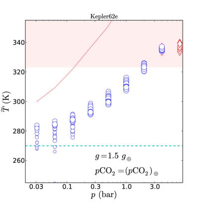
Figure 4: Influence of planetary parameters not constrained by observations on the mean global surface temperature, $\widetilde{T}$, of Kepler62-e. Symbols: predictions of ESTM simulations plotted as a function of surface pressure, $p$, for all possible combinations of rotation rate, axis obliquity and ocean fraction described in §4.1.1. Circles: habitable solutions. Diamonds: solutions with water vapor column above the critical limit discussed in §A. The symbol size scales with the fractional habitability, $h_{\text{lw}}$. Left: Earth atmospheric composition. Right: Earth-like atmospheric composition with a one hundred-fold increase of $p$CO₂. Dashed line: equilibrium temperature of Kepler62-e (Borucki, 2013). Dotted line: water boiling point as a function of $p$.

4 Applications

After the calibration and validation, we apply the model to explore the dependence of $T(\varphi,t)$ and the mean global surface temperature, $\widetilde{T}$, on a variety of planet parameters. At variance with the validation tests, we now consider all the features of the model, including the ice-albedo feedback.In Appendix C we present simulations of idealized Earth-like planets. Here we describe a test study of exoplanet habitability.

4.1 Exoplanets

The modelization of the surface temperature of exoplanets is severely constrained by the limited amount of observational data. Typically, one can measure the stellar and orbital parameters and a few planetary quantities, such as the radius and/or mass. From the stellar and orbital data one can estimate the planet insolation and its seasonal evolution. From the radius and mass one can estimate the surface gravity which enters in the parameterization of the atmospheric columnar mass. Unfortunately, many planet quantities that are required for the modelization are currently not observable. These include the atmospheric composition, surface pressure, ocean/land distribution, axis obliquity and rotation period. Taking advantage of the flexibility of the ESTM, we can perform a fast exploration of the space of the unknown quantities, treating them as free parameters. From the application of this methodology we can assess the relative importance in terms of climate impact of the planet quantities that are not measurable. In addition, we can constrain the ranges of parameters values that yield habitable solutions.

We show two examples of application of this methodology. First we consider a specific exoplanet chosen as a test case, then we introduce a statistical ranking of planetary habitability. We adopt an index of habitability, $h_{\text{lw}}$, based on the liquid water criterion.

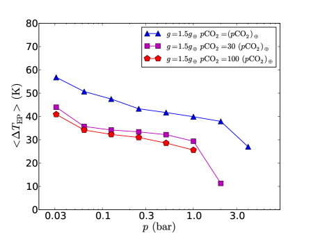
Figure 5: Average equator-pole temperature difference, ${\textstyle<}\Delta T_{\text{EP}}{\textstyle>}$, obtained from ESTM simulations of Kepler62-e (§4.1.1), plotted as a function of surface pressure, $p$. Each curve is calculated at constant $p$CO₂, as specified in the legend.

4.1.1 Kepler-62e as a test case

The test-case exoplanet was chosen using three criteria. The first is that the planet should be of terrestrial type, i.e. rocky and without an extended atmosphere, in order to be suitable for the application of the ESTM. We used the radius for a preliminary characterization of the planet, since evidence is accumulating for the existence of a gradual transition, correlated with radius, between planets of terrestrial type and planets with rocky cores but extended gas envelopes (e.g. Wu & Lithwick, 2013; Marcy, 2014). We restricted our search to planets with $R\lesssim 1.7R_{\oplus}$, the threshold for terrestrial planets found in a statistical study of size, host-star metallicity and orbital period (Buchhave et al., 2014). As a second criterion, we required the orbital semimajor axis to be larger than the tidal lock radius, since the ESTM  cannot be applied to tidally locked planets. Finally, given the extreme dependence of habitability on insolation (see e.g. Fig. 10), we selected planets with an insolation within $\pm 50\%$ of the present-day Earth value. By querying the Exoplanet Orbit Database (Wright, 2011) at exoplanets.org, we found that only Kepler-62 e (Borucki, 2013) satisfies the above criteria. The radius, $R=1.61R_{\oplus}$, and orbital period, $P=122\,$d, suggest that Kepler-62 e is probably of terrestrial type (see Buchhave et al., 2014, Fig. 2). Its insolation is only 19% higher than the Earth’s value, and its semimajor axis, $a=0.427$ AU, is larger than the tidal lock radius, $r_{\mathrm{tl}}=0.31$ AU.

To run the ESTM simulations of Kepler-62e we adopted at face value the radius, semimajor axis, eccentricity and stellar flux provided by the observations (Borucki, 2013). Unfortunately, only a loose upper limit ($M<36\,M_{\oplus}$) is available for the mass, so that the surface gravity $g$ is poorly constrained at the present time. For illustrative purposes, we adopt $g=1.5\,g_{\oplus}$ ($M=3.9\,M_{\oplus}$), corresponding to a mean density $5.1$ g cm^-3, similar to that of the Earth ($\rho_{\oplus}=5.5$ g cm^-3). As far as the atmosphere is concerned, we vary the surface pressure in the range $p\in(0.03,8)$ bar and the CO₂ partial pressure in the range $p$CO₂/($p$CO₂)${}_{\oplus}\in(1,100)$. We adopt 3 representative values of rotation rate, $\Omega/\Omega_{\oplus}\in(0.5,1,2)$, axis obliquity, $\epsilon\in(0^{\circ},22.5^{\circ},45^{\circ})$, and ocean coverage, $f_{o}\in(0.5,0.75,1.0)$. For the remaining parameters we adopt the Earth’s reference values. For each value of CO₂ partial pressure we run simulations covering all possible combinations of background pressure, rotation rate, axis obliquity and ocean coverage listed above. Part of the results of these simulations are shown in Figs. 4 and 5.

In Fig. 4 we plot the mean global temperature, $\widetilde{T}$, obtained for two different values of $p$CO₂, specified in the legends. At each value of $p$, we show the values of $\widetilde{T}$ obtained from all possible combinations of $\Omega$, $\epsilon$, and $f_{o}$. The typical scatter of $\widetilde{T}$ due a random combination of these 3 parameters is $\simeq$ 10-20 K. On top of this scatter, the most remarkable feature is a positive trend of $\widetilde{T}$ versus $p$ extending over an interval of $\approx 60$ K. Within the limits of application of the model, these results indicate that an uncertainty on $p$ within the range expected for terrestrial planets has stronger effects on $\widetilde{T}$ than uncertainties of rotation rate, axis obliquity and ocean coverage. In fact, variations of $p$ have strong effects both on $T(\varphi,t)$ and $\widetilde{T}$ because they are equivalent to variations of atmospheric columnar mass, $p/g$, which affect both the latitudinal transport (i.e. the surface temperature distribution), and the radiative transfer (i.e. the global energy budget).

The results shown in Fig. 4 constrain the interval of $p$ that allows Kepler-62e to be habitable. At high $p$, the habitability is limited by the rise of $\widetilde{T}$, which eventually leads to a runaway greenhouse instability. The red diamonds in Fig. 4 indicate cases where the water vapor column exceeds the critical value that we tentatively adopt as a limit for the onset of such instability (§A). At low $p$, two factors combine to limit the habitability. One is the onset of large temperature excursions and the other the decrease of the water boiling point (dotted lines in Fig. 4). As a result, the fraction of planet surface outside the liquid water temperature becomes larger at low $p$. To evidentiate this effect, we have scaled the size of the symbols in Fig. 4 according to the value of $h_{\text{lw}}$. One can see that $h_{\text{lw}}$ tends to become smaller at low $p$, especially when $\widetilde{T}$ approches the temperature regime where the ice-albedo feedback becomes important. In some cases, not shown in the figure, the planet undergoes a complete snowball transition and the habitability becomes zero. The effect of temperature excursions is shown in Fig. 5, where we plot as a function of $p$ the average value of $\Delta T_{\text{EP}}$ obtained from all possible combinations of $\Omega$, $\epsilon$, and $f_{o}$. One can see that the temperature excursions become large with decreasing level of CO₂; this happens because at low CO₂ the temperature is sufficiently low for the development of the ice-albedo feedback, and because the lowered IR optical depth of the atmosphere is less effective in reducing the effect of the geometrically-induced meridional insolation variation at the surface.

Fig. 4 shows that the equilibrium temperature of Kepler-62e, $T_{\text{eq}}=270\pm 15$ K (Borucki, 2013, dashed line), lies at the lower end of the predicted $\widetilde{T}$ values. The difference $\widetilde{T}-T_{\mathrm{eq}}$ increases with atmospheric columnar mass because the estimate of $T_{\mathrm{eq}}$ does not consider the greenhouse effect.

Figure 6: Ranking index of habitability, $r_{h}$, obtained from ESTM simulations of Kepler-62e and an Earth twin (§4.1.2) plotted as a function of surface pressure, $p$. Symbols for Kepler-62e as in Fig. 5. Crossed circles: Earth twin.

4.1.2 Statistical ranking of planetary habitability

By performing a large number of simulations for a wide combination of parameters we can quantify the habitability in a statistical way. To illustrate this possibility with an example we consider again the test case of Kepler-62e. We perform a statistical analysis of the results obtained from all combinations of $\Omega$, $\epsilon$, and $f_{o}$ values adopted at a given $p$. We tag as “non habitable” the cases with a snowball transition and those with a critical value of water vapor. For each set of parameters {$\Omega$, $\epsilon$, $f_{o}$} we count the number of cases that are found to be habitable, $n_{h}$, over the total number of simulations, $n_{t}$. From this we calculate the fraction $\psi_{h}=n_{h}/n_{t}$, which represents the probability for the planet to be habitable if the adopted parameter values are equally plausible a priori. We then call ${\textstyle<}h_{\text{lw}}{\textstyle>}=(1/n_{h})\sum_{i=1}^{n_{h}}(h_{\text{lw}})_{i}$ the mean surface habitability of the $n_{h}$ sets that yield a habitable solution. At this point we define a “ranking index of habitability”

$$r_{h}\equiv\psi_{h}\times{\textstyle<}h_{\text{lw}}{\textstyle>}={1\over n_{t}}\sum_{i=1}^{n_{h}}\,(h_{\text{lw}})_{i}~{}~{}.$$ (31)

This index takes into account at the same time the probability that the planet is habitable and the average fraction of habitable surface. As an example, in Fig. 6 we plot $r_{h}$ versus $p$ for the different values of $p$CO₂ considered in our simulations of Kepler-62e. One can see that $r_{h}\simeq 1$ only in a limited range of surface pressure. At very low pressure, the index becomes lower because the fraction of habitable surface decreases and because $\psi_{h}$ drops below unity when a snowball transition is encountered. At high pressure $\psi_{h}$ drops when the water vapor limit is encountered. As an example of application, we can constrain the interval of $p$ suitable for the habitability of Kepler62-e. For $p$CO₂= ($p$CO₂)_⊕ (triangles) the requirement of habitability yields the limit $p\lesssim 3$ bar. As $p$CO₂ increases (squares and pentagons), the upper limit becomes more stringent ($p\lesssim 1$ bar), but the planet has a higher probability of being habitable at relatively low pressure.

Clearly, the index $r_{h}$ does not have an absolute meaning since its value depends on the choice of the set of parameters. However, by choosing a common set, the index $r_{h}$ can be used to rank the relative habitability of different planets. As an example, in Fig. 6 we plot $r_{h}$ versus $p$ obtained for an Earth twin with the same sets of parameters {$\Omega$, $\epsilon$, $f_{o}$} adopted for Kepler-62e. One can see that at $p\gtrsim 1$ bar the Earth twin (crossed circles) is more habitable than Kepler-62e for the adopted set of parameters, while at $p\lesssim 1$ bar Kepler-62 is more habitable than the Earth twin.

5 Summary and conclusions

We have assembled the ESTM set of climate tools (Figure 1) to model the latitudinal and seasonal variation of the surface temperature, $T(\varphi,t)$, on Earth-like planets. The motivation for building the ESTM is twofold. From the general point of view of exoplanet research, Earth-size planets are expected to be rather common, but difficult to characterize with experimental methods. From the astrobiological point of view, Earth-like planets are excellent candidates in the quest for habitable environments. A fast simulation of $T(\varphi,t)$ enables us to characterize the surface properties of these planets by sampling the wide parameter space representative of the physical quantities not measured by observations. The detailed modelization of the surface temperature is essential to estimate the habitability of these planets using the liquid water criterion or a proper set of thermal limits of life (e.g. Clarke, 2014).

The ESTM consists of an upgraded type of EBM featuring a multi-parameter description of the physical quantities that dominate the vertical and horizontal energy transport (Fig. 1). The functional dependence of the physical quantities is derived using single-column atmospheric calculations and algorithms tested with 3D climate experiments. Special attention has been dedicated to improve (§2.1) and validate (§3.1) the description of the meridional transport, a weak point of classic EBMs. The functional dependence of the meridional transport on atmospheric columnar mass and rotation rate is significantly milder [see Eq. (23)] than the one adopted in previous EBMs. The reference Earth model obtained from the calibration process is able to reproduce with accuracy the average surface temperature properties of the Earth and to capture the main features of the Earth albedo and meridional energy transport (Figs. 7 and 8). Once calibrated, the ESTM is able to reproduce the mean equator-pole temperature difference, $\Delta T_{\text{EP}}$, predicted by 3D aquaplanet models (Fig. 3).

The ESTM simulations provide a fast “snapshot” of $T(\varphi,t)$ and temperature-based indices of habitability for any set of input parameters that yields a stationary solution. The planet parameters that can be changed include radius, $R$, surface pressure, $p$, gravitational acceleration, $g$, rotation rate, $\Omega$, axis tilt, $\epsilon$, ocean/land coverage and partial pressure of non-condensable greenhouse gases. The approximate limits of validity of the present version of the ESTM can be summarized as follows: $0.5\lesssim R/R_{\oplus}\lesssim 2$, $p\lesssim 10$ bar, $0.5\lesssim\Omega/\Omega_{\oplus}\lesssim 5$, $\epsilon\lesssim 45^{\circ}$; $p$CO₂ and $p$CH$4$ can be changed, but should remain in trace abundances with respect to an Earth-like atmospheric composition. The requirement of a relatively high rotation rate is inherent to the simplified treatment of the horizontal transport. However, the ESTM can be applied to explore the early habitability of slow rotating planets that had an initial fast rotation.

We have performed ESTM simulations of idealized Earth-like planets to evaluate the impact on the planet temperature and habitability resulting from variations of rotation rate, insolation, atmospheric columnar mass, radius, axis obliquity, ocean/land distribution, and long-wavelength cloud forcing (Figs. 9 - 15). Most of these quantities can easily induce $\sim 30$-$40$% changes of the mean annual habitability for parameter variations well within the range expected for terrestrial planets. Variations of insolations within $\pm 10\%$ of the Earth value can impact the habitability up to $100\%$. The land/ocean distribution mainly affects the seasonal habitability, rather than its mean annual value. The impact of rotation rate is weaker than predicted by classic EBMs, without evidence of a snowball transition at $\Omega/\Omega_{\oplus}\gtrsim 3$. A general result of these numerical experiments is that the ice-albedo feedback amplifies changes of $T(\varphi,t)$ resulting from variations of planet parameters.

We have tested the capability of the ESTM to explore the habitability of a specific exoplanet in presence of a limited amount of observational data. For the exoplanet chosen for this test, Kepler-62e, we used the stellar flux, orbital parameters and planet radius provided by the observations (Borucki, 2013), together with a surface gravity $g=1.5\,g_{\oplus}$ adopted for illustrative purposes. We treated the surface pressure, $p$CO₂, rotation rate, axis tilt and ocean coverage as free parameters. We find that $\widetilde{T}$ increases from $\approx 280$ K to $\approx 340$ K when the surface pressure increases between $p\simeq 0.03$ bar and $3$ bar; this trend dominates the scatter of $\simeq 10$-20 K resulting from variations of rotation rate, axis tilt and ocean coverage at each value of $p$. We also find that the surface pressure of Kepler-62e should lie above $p\approx 0.05$ bar to avoid the presence of a significant ice cover and below $\approx 2$ bar to avoid the onset of a runaway greenhouse instability; this upper limit is confirmed for different values of $p$CO₂ and surface gravity. These results demonstrate the ESTM capability to evaluate the climate impact of unknown planet quantities and to constrain the range of values that yield habitable solutions. The test case of Kepler-62e also shows that the equilibrium temperature commonly published in exoplanet studies represents a sort of lower limit to the mean global temperature of more realistic models.

We have shown that the flexibility of the ESTM makes it possible to quantify the habitability in a statistical way. As an example, we have introduced a ranking index of habitability, $r_{h}$, that can be used to compare the overall habitability of different planets for a given set of reference parameters (§4.1.2). For instance, we find that at $p\lesssim 1$ bar Kepler-62e is more habitable than an Earth twin for the combination of rotation rates, axis tilts and ocean fractions considered in our test, whereas the comparison favours the Earth twin at $p\gtrsim 1$ bar. The index $r_{h}$ can be applied to select the best potential cases of habitable exoplanets for follow-up searches of biomarkers.

The results of this work indicate the level of accuracy required to estimate the surface habitability of terrestrial planets. The quality of exoplanet orbital data and host star fluxes should be improved to measure the insolation with an accuracy of $\approx 1\%$. In spite of the difficulty of characterizing terrestrial atmospheres (e.g., Misra et al., 2013), an effort should be made to constrain the atmospheric pressure, possibly within a factor of two.

Appendix A Running the simulations

The ESTM simulations consist in a search for a stationary solution $T(\varphi,t)$ of Eq. (1). We solve the spatial derivates with the Euler method, with the boundary condition that the flux of horizontal heat into the pole vanishes. The temporal derivates are solved with the Runge-Kutta method. The solution is searched for by iterations, starting with an assigned initial value of temperature equal in each zone, $T(\varphi,t_{\circ})\equiv T_{\mathrm{start}}$. Every 10 orbits we calculate the mean global orbital temperature, $\widetilde{T}$. The simulation is stopped when $\widetilde{T}$ converges within a prefixed accuracy. In practice, we calculate the increment $\delta\widetilde{T}$ every 10 orbits and stop the simulation when $|\delta\widetilde{T}|<0.01$ K. In most cases the convergence is achieved in fewer than 100 orbits. After checking that the simulations converge to the same solution starting from widely different values of $T_{\mathrm{start}}>273$ K, we adopted $T_{\mathrm{start}}=275$ K. The choice of this “cold start” allows us to study atmospheres with very low pressure, where the boiling point is just a few kelvins above the freezing point; in these cases, the adoption of a higher $T_{\mathrm{start}}$ would force most of the planet surface to evaporate at the very start of the simulation. The adoption of a lower $T_{\mathrm{start}}$, on the other hand, would trigger artificial episodes of glaciation.

In addition to the regular exit based on the convergence criterion, we interrupt the simulation in presence of water vapor effects that may lead to a condition of non-habitability. Specifically, two critical conditions are monitored in the course of the simulation. The first takes place when $T(\varphi,t)$ exceeds the water boiling point, $T_{\mathrm{b}}$. The second, when the columnar mass of water vapour exceeds 1/10 of the total atmospheric columnar mass (see next paragraph). In the first case, the long term habitability might be compromised due to evaporation of the surface water. The second condition might lead to the onset of a runaway greenhouse instability (Hart, 1978; Kasting, 1988) with a complete loss of water from the planet surface. The ESTM does not track variations of relative humidity and is not suited to describe these two cases. By interrupting the simulation when one of these two conditions is met, we limit the range of application of the simulations to cases with a modest content of water vapor that can be safely treated by the model.

The limit of water vapor columnar mass that we adopt is inspired by the results of a study of the Earth climate variation induced by a rise of insolation (Leconte et al., 2013). When the insolation attains 1.1 times the present Earth value, the 3D moist model of Leconte et al. (2013) predicts an energy unbalance that would lead to a runaway greenhouse instability. The mixing ratio of water vapor over moist air predicted at the critical value of insolation is $\simeq 0.1$ (Leconte et al., 2013, Fig. 3b). The limit of water columnar mass that we adopt is based on this mixing ratio.

For the simulations presented in this work, we adopt a grid of $N=54$ latitude zones. The orbital period is sampled at $N_{s}=48$ instants of time to investigate the seasonal evolution of the surface quantities of interest (e.g. temperature, albedo, ice coverage). With this set-up, the simulation of the Earth model presented below attains a stationary solution after 50 orbital periods, with a CPU time of $\sim 70$ s on a 2.3 GHz processor. This extremely high computational efficiency is the key to perform the large number of simulations required to cover the broad parameter space of exoplanets.

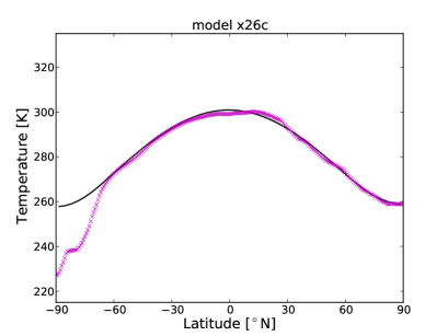
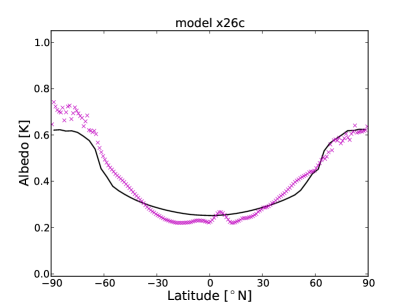
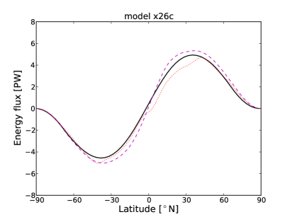
Figure 7: Mean annual latitude profiles of surface temperature, albedo and meridional energy flux predicted by the reference Earth model (solid line). Top panel: the temperature profile is compared with ERA Interim 2m temperatures (Dee, 2011) averaged in the period 2001-2013 (crosses). Middle panel: the albedo profile is compared with CERES short-wavelength albedo (Loeb et al., 2005, 2007) averaged in the same period (crosses). Bottom panel: the meridional energy flux profile is compared with the total (dashed line) and atmospheric (dotted line) profiles obtained from the EC-Earth model (Hazeleger et al., 2010).

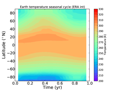
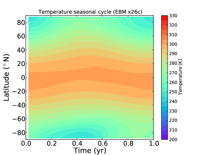
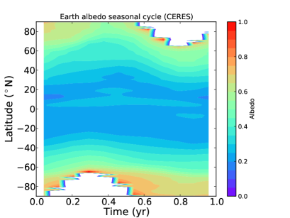
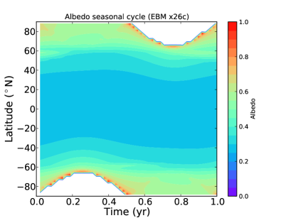
Figure 8: Seasonal and latitudinal variations of surface temperature (top panels) and top-of-atmosphere albedo (bottom panels) of the Earth. Left panels: average ERA Interim 2m temperatures (Dee, 2011) and CERES short-wavelength albedo (Loeb et al., 2005, 2007) in the years 2001-2013. Right panels: predictions of the reference Earth model. The zero point of the time scale is set at the spring equinox. Blank areas in the albedo panels indicate regions of the seasonal-latitudinal space without incident stellar flux.

Appendix B The reference Earth model

For the calibration of the reference Earth model we adopted orbital parameters, axis tilt, and rotation period from Cox (2000). For the solar constant we adopted $S_{0}=1360$ W m^-2 and $g=9.8$ m s^-2 for the surface gravity acceleration. The zonal coverage of continents and oceans was taken from Table III in WK97. We adopted a relative humidity $q=0.6$ (see §2.2) and volumetric mixing ratios of CO₂ and CH₄ of 380 ppmV and 1.8 ppmV, respectively. The surface pressure of dry air, $p_{\mathrm{dry}}=1.0031\times 10^{5}$ Pa, was tuned to match the moist surface pressure of the Earth, $p_{\mathrm{tot}}=1.0132\times 10^{5}$ Pa. The remaining parameters of the model are shown in Table 1. Some parameters were fine tuned to match the mean annual global quantities of the northern hemisphere of the Earth, as specified in the Table. We avoided using the southern hemisphere as a reference since its climate is strongly affected by the altitude of Antartica, while orography is not included in the model. In Table 2, column 3, we show the experimental data of the northern hemisphere used as a guideline to tune the model parameters. In column 4 of the same table we show the corresponding predictions of the Earth reference model.

In Fig. 7 we show the mean annual latitude profiles of surface temperature, top-of-atmosphere albedo and meridional energy flux predicted by the reference model (solid line). The temperature profile is compared with ERA Interim 2m temperatures (Dee, 2011) averaged in the period 2001-2013 (crosses in the top panel). Area-weighted temperature differences between observed and predicted profile have an rms of 1.1 K in the northern hemisphere. The albedo profiles are compared with the CERES short-wavelength albedo (Loeb et al., 2005, 2007) averaged in the same period (crosses in the middle panel). The ESTM is able to reproduce reasonably well the rise of albedo with increasing latitude. This rise is due to two factors: the dependence of the atmosphere, ocean, and cloud albedo on zenith distance (§§2.2.2,2.3.3) and the increasing coverage of ice at low temperature (§2.3.1). The meridional flux in the bottom panel is compared with the total flux (dashed line) and the atmospheric flux (dotted line) obtained from EC-Earth model (Hazeleger et al., 2010). In spite of the simplicity of the transport formalism intrinsic to Eq. (1), the model is able to capture remarkably well the latitude dependence of the meridional transport.

The seasonal variations of the temperature and albedo latitudinal profiles are compared with the experimental data in Fig. 8. One can see that the reference model is able to capture the general patterns of seasonal evolution.

Even if the reference model has been tuned using northern hemisphere data, the predictions shown in Figs. 7 and 8 are in general agreement with the data also for most the southern hemisphere, with the exception of Antartica. It is remarkable that the atmospheric transport in both hemispheres is reproduced well, in spite of significant differences in the ocean contribution between the two hemispheres (see §2.1.3).

Once the reference model is calibrated, some of the parameters that have been tuned to fit the present-day Earth’s climate can be changed for specific applications of the ESTM to exoplanets. As an example, even if we adopt $a_{s}=0.18$ for the surface albedo of continents in the reference model, we may adopt lower values, typical of forests, or higher values, typical of sandy deserts, for specific applications. More information on the parameters that can be changed is given in Table 1.

Appendix C Model simulations of idealized Earth-like planets

In this set of experiments we study the effects of varying a single planet quantity while assigning Earth’s values to all the remaining parameters. We consider variations of rotation period, insolation, atmospheric columnar mass, radius, obliquity, land distribution, and long-wavelength cloud forcing.

C.1 Rotation rate

In Fig. 9 we show how $T(\varphi,t)$ is affected by variations of rotation rate, the left and right panel corresponding to the cases $\Omega=0.5\,\Omega_{\oplus}$ and $\Omega=4\,\Omega_{\oplus}$, respectively. One can see that the change of the surface temperature distribution is quite dramatic in spite of the modest dependence of the transport coefficient on rotation rate that we adopt, $D\propto\Omega^{-4/5}$ [see Eq.(21)]. The mean global habitability changes from $h_{\text{lw}}=0.94$ in the slow-rotating case to $h_{\text{lw}}=0.71$ in the fast-rotating case. The corresponding change of mean global temperature is relatively small, from $\widetilde{T}=284$ K to 290 K. These results show the importance of estimating $T(\varphi,t)$, rather than $\widetilde{T}$, in order to quantify the habitability.

The behavior of the mean equator-pole difference, $\Delta T_{\text{EP}}$, is useful to interpret the results of this test. We find $\Delta T_{\text{EP}}=28$ K in the slow-rotating case and $\Delta T_{\text{EP}}=80$ K in the fast-rotating case. This variation of $\Delta T_{\text{EP}}$ is much higher than that found for the same change of rotation rate in the case of the KS14 aquaplanet (top-left panel in Fig. 3). We interpret this strong variation of $\Delta T_{\text{EP}}$ in terms of the ice-albedo feedback, which is positive and tends to amplify variations of the surface temperature. This feedback is accounted for in the present experiment, but not in the case of the aquaplanet. These results illustrate the importance of using climate models with latitude temperature distribution and ice-albedo feedback in order to estimate the fraction of habitable surface.

The analysis of the ice cover evidentiates another important difference between the ESTM and classic EBMs. With the ESTM the ice cover increases from $\simeq 3\%$ at $\Omega=0.5\,\Omega_{\oplus}$ to $\simeq 23\%$ at $\Omega=4\,\Omega_{\oplus}$. This increase is less dramatic than the transition to a complete “snowball” state (i.e. ice cover $\simeq 100\%$) found with classic EBMs at $\Omega=3\,\Omega_{\oplus}$ (e.g. Spiegel et al., 2008). This difference is due to two factors. One is the strong dependence of the transport on rotation rate adopted in most EBMs ($D\propto\Omega^{-2}$), which is not supported by the validation tests discussed above (top-left panel of Fig. 3). Another factor is the algorithm adopted for the albedo, which in classic EBMs is a simple analytical function $A=A(T)$, while in the ESTM is a multi-parameter function $A=A(T,p,g,p\mathrm{CO_{2}},a_{\mathrm{s}},Z)$ that takes into account the vertical transport of stellar radiation (§2.2.2). These results show the importance of adopting algorithms calibrated with 3D experiments and atmospheric column calculations.

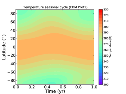
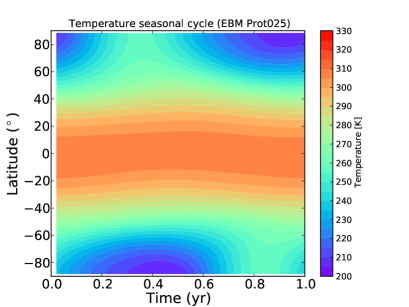
Figure 9: Variation of surface temperature as a function of latitude and orbital phase for an Earth-like planet with rotation rate $\Omega=0.5\,\Omega_{\oplus}$ (left) and $\Omega=4\,\Omega_{\oplus}$ (right). All the remaining parameters are those used for the Earth reference model (Appendix B).

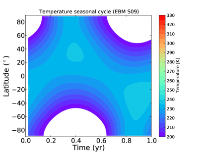
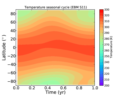
Figure 10: Variation of surface temperature as a function of latitude and orbital phase for an Earth-like planet with insolation 10% lower (left) and 10% higher (right) than the present-day value. All the remaining parameters are those used for the Earth reference model (Appendix B). Blank areas in the left panel indicate regions of the $(\varphi,t)$ space with surface temperature below 200 K.

C.2 Insolation

In Fig. 10 we show how $T(\varphi,t)$ is affected by variations of stellar insolation, the left and right panel corresponding to an insolation of 0.9 and 1.1 times the present-day Earth’s insolation ($S/4\simeq 341$ W m^-2), respectively. In the first case the ESTM finds a complete snowball with $\widetilde{T}=223$ K and $h_{\text{lw}}=0$, while in the latter $\widetilde{T}=306$ K and $h_{\text{lw}}=1$ with no ice cover. These results demonstrate the extreme sensitivity of the surface temperature to variations of insolation and the need of incorporating feedbacks in global climate models in order to define the limits of insolation of a habitable planet.

Our model is able to capture the ice-albedo feedback, but is not suited for treating hot atmospheres and the runaway greenhouse instability. To test the limits of the ESTM we have gradually increased the insolation and compared our results with those obtained by the 3D model of Leconte et al. (2013). We found that the ESTM tracks the rise of $\widetilde{T}$ with insolation predicted by the 3D model up to $S/4\simeq 365$ W m^-2. At higher insolation, the 3D model predicts a faster rise of $\widetilde{T}$ due to an increase of the radiative cloud forcing.

By decreasing the insolation with respect to the Earth’s value, the ESTM finds solutions characterized by increasing ice cover. At $S/4\simeq 310$ W m^-2 the simulation displays a runaway ice-albedo feedback that leads to a complete snowball configuration. This result sets the ESTM limit of minimum insolation for the liquid-water habitability of an Earth-twin planet.

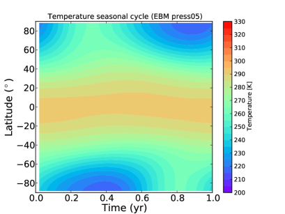
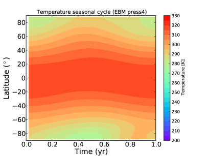
Figure 11: Variation of surface temperature as a function of latitude and orbital phase for an Earth-like planet with surface pressure $p=0.5$ bar (left) and $4$ bar (right). All the remaining parameters are those used for the Earth reference model (Appendix B).

C.3 Atmospheric columnar mass

In Fig. 11 we show how $T(\varphi,t)$ is affected by variations of surface pressure, the left and right panel corresponding to the cases $p=0.5$ bar and $4$ bar, respectively. Since the surface gravity is kept fixed at $g=g_{\oplus}$, this experiment also investigates the climate impact of variations of atmospheric columnar mass, $p/g$. We find a significant difference in mean temperature and habitability between the two cases, with $\widetilde{T}=274$ K and $h_{\text{lw}}=0.62$ in the low-pressure case and $\widetilde{T}=310$ K and $h_{\text{lw}}=1.00$ in the high-pressure case. The mean equator-pole difference, decreases from $\Delta T_{\text{EP}}=$55 K to 33 K between the two cases. The rise of mean temperature is due to the existence of a positive correlation between columnar mass and intensity of the greenhouse effect. The decrease of temperature gradient results from the correlation between $p/g$ and the efficiency of the horizontal transport. Both effects have been already discussed in Paper I. Here we find a more moderate trend with $p/g$, as a result of the new formulation of $D$ that we adopt.

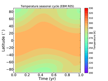
Figure 12: Variation of surface temperature as a function of latitude and orbital phase for an Earth-like planet with radius $R=0.5\,R_{\oplus}$ (left) and $1.5\,R_{\oplus}$ (right). The mean density of the planet is assumed to be constant, $\rho=\rho_{\oplus}$, so that the same model predictions are also appropriate for an Earth-like planet with mass $M=0.125\,M_{\oplus}$ (left panel) and $3.375\,M_{\oplus}$ (right panel). The atmospheric columnar was kept constant by scaling $p$ and $g$ with $R$. All the remaining parameters are those used for the Earth reference model (Appendix B).

C.4 Planet radius or mass

In Fig. 12 we show how $T(\varphi,t)$ is affected by variations of planet radius, the left and right panel corresponding to the cases $R=0.5\,R_{\oplus}$ and $1.5\,R_{\oplus}$, respectively. In this ideal experiment we keep fixed the planet mean density, $\rho=\rho_{\oplus}$, so that the planet mass and gravity scale as $M\propto R^{3}$ and $g\propto R$, respectively. We also keep fixed the columnar mass, $p/g=(p/g)_{\oplus}$, by scaling $p$ and $g$ with $R$. With this experimental setup, the radius is the only parameter that varies in the transport coefficient $D$ [Eqs. (23), (24), and (25)]. The left panel corresponds to the case $M=0.125\,M_{\oplus}$, $p=0.5$ bar and $g=0.5\,g_{\oplus}$ and the right panel to the case $M=3.375\,M_{\oplus}$, $p=1.5$ bar and $g=1.5\,g_{\oplus}$.

We find that the planet cools significantly when the radius, mass and gravity increase, with a variation of the mean global temperature from $\widetilde{T}=294$ K to 281 K. The equator-to-pole temperature differences increases dramatically, from $\Delta T_{\text{EP}}=$18 K to 64 K, respectively. This change of $\Delta T_{\mathrm{PE}}$ is much higher than that found for the same change of radius in the case of the aquaplanet (bottom-right panel in Fig. 3). The inclusion of the ice-albedo feedback in the present experiment amplifies variations of $\Delta T_{\mathrm{PE}}$. In fact, the ice cover increases from 0% to 21% between $R=0.5\,R_{\oplus}$ and $1.5\,R_{\oplus}$. As a result of the variations of $\widetilde{T}$ and $\Delta T_{\text{EP}}$, the mean global habitability is significantly affected, changing from $h_{\text{lw}}=1.00$ to 0.71 with increasing planet size.

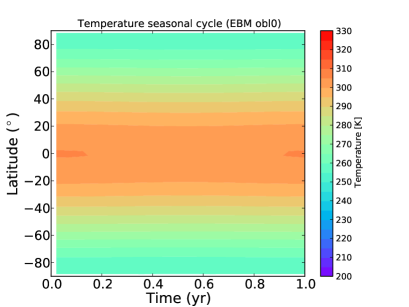
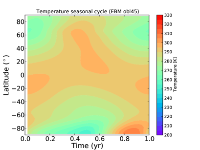
Figure 13: Variation of surface temperature as a function of latitude and orbital phase for an Earth-like planet with axis obliquity $\epsilon=0^{\circ}$ (left) and $45^{\circ}$ d (right). All the remaining parameters are those used for the Earth reference model (Appendix B).

C.5 Axis obliquity

In Fig. 13 we show how $T(\varphi,t)$ is affected by variations of axis obliquity, the left and right panel corresponding to the cases $\epsilon=0^{\circ}$ and $45^{\circ}$, respectively. We find a modest decrease of $\widetilde{T}$, from $291$ K to 289 K, and a significant decrease of $\Delta T_{\text{EP}}$, from 42 K to 15 K. The mean annual temperature at the poles is lower at $\epsilon=0^{\circ}$ than at $\epsilon=45^{\circ}$, because in the first case the poles have a constant, low temperature, while in the latter they alternate cool and warm seasons. As a result, the ice cover decreases and the habitability increases in the range from $\epsilon=0^{\circ}$ to $\epsilon=45^{\circ}$ For the conditions considered in this experiment, the initial ice cover is relatively small ($\simeq 7\%$) and the increase of habitability relatively modest (from $0.87$ to 0.95). Larger variations of habitability are found starting from a higher ice cover. These results confirm the necessity of determining $T(\varphi,t)$ and accounting for the ice-albedo feedback in order to estimate the habitability.

At $\epsilon>45^{\circ}$ EBM studies predict a stronger climate impact of obliquity, with possible formation of equatorial ice belts (Williams & Kasting, 1997; Spiegel et al., 2009; Vladilo et al., 2013). The physically-based derivation of the coefficient $D$ prevents using the ESTM when the equatorial-polar gradient is negative, because Eqs. (21) and (23) require $\delta T>0$. In the Earth model this condition is satisfied when $\epsilon\leq 52^{\circ}$. Clearly, the climate behavior at high obliquity should be tested with 3D climate experiments (e.g. Williams & Pollard, 2003; Ferreira et al., 2014, and refs. therein), being cautious with predictions obtained with EBMs.

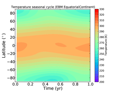
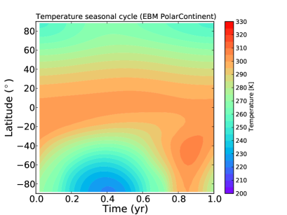
Figure 14: Variation of surface temperature as a function of latitude and orbital phase for an Earth-like planet with global ocean coverage of 0.7 and a single continent covering the remaining surface. Left panel: equatorial continent spread over all longitudes. Right panel: polar continent centered at latitude $-90^{\circ}$. All the remaining parameters are those used for the Earth reference model (Appendix B).

C.6 Ocean/land distribution

In Fig. 14 we show how $T(\varphi,t)$ is affected by variations of the geographical distribution of the continents. In these experiments we consider a single continent covering all longitudes, but located at different latitudes in each case. The global ocean coverage is fixed at 0.7, as in the case of the Earth. In the left panel we show the the case of a continent centered on the equator, while in the right panel a continent centered on the southern pole. The variation of $T(\varphi,t)$ is quite remarkable given the little change of mean global annual temperature ($\widetilde{T}=288$ K and 289 K for the equatorial and polar case, respectively). The mean annual habitability is almost the same in the two continental configurations ($0.86$ and $0.85$), but in the case of the polar continent the fraction of habitable surface shows strong seasonal oscillations. This behaviour is due to the low thermal capacity of the continents and the large excursions of polar insolation.

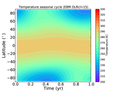
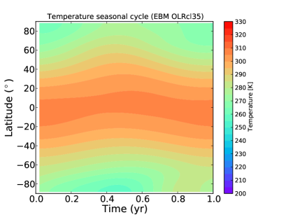
Figure 15: Variation of surface temperature as a function of latitude and orbital phase for an Earth-like planet with long-wavelength cloud forcing 15 W/m² (left) and 35 W/m² (right). All the remaining parameters are those used for the Earth reference model (Appendix B).

C.7 Long-wavelength cloud forcing

In Fig. 15 we show how $T(\varphi,t)$ is affected by variations of the long-wavelength forcing of clouds. Analysis of Earth data indicates a mean value 26.4 W/m² (Stephens et al., 2012), but with large excursions (e.g. Hartmann et al., 1992). To illustrate the impact of this quantity on the surface temperature we have adopted $15$ W/m² (left panel) and $35$ W/m² (right panel) since this range brackets most of the Earth values. The impact on the mean global temperature is relatively high, with a rise from $\widetilde{T}=277$ K to 295 K between the two cases. The ice cover correspondingly decreases from 24% to 2%, while the habitability increases from $h_{\text{lw}}=0.68$ to 0.95. The mean equator-pole temperature difference shows a decrease from $\Delta T_{\text{EP}}=52$ K to 36 K. This decrease of $\Delta T_{\text{EP}}$ is more moderate than found for variations of rotation rate, radius and axis tilt.

Table 1: Fiducial parameters of the ESTM

Parameter	Fiducial value	Description	References/Comments
$C_{\text{ml50}}$	$210\times 10^{6}$ J m-2 K-1	Thermal inertia of the oceans${}^{\text{a}}$ (§2.3.4)	Pierrehumbert (2010)
$C_{\text{atm},\circ}$	$10.1\times 10^{6}$ J m-2 K-1	Thermal inertia of the atmosphere${}^{\text{a}}$ (§2.3.4)	Pierrehumbert (2010)
$C_{\text{solid}}$	$1\times 10^{6}$ J m-2 K-1	Thermal inertia of the solid surface(§2.3.4)	Vladilo et al. (2013)
$D_{\circ}$	0.66 W m-2 K-1	Coefficient of latitudinal transport (§2.1.1)	Tunedb to match $T$-latitude profile (Fig. 7)
$\mathcal{R}$	2.2	Modulation of latitudinal transport (§2.1.2)	Tuned to match $T$-latitude profile (Fig. 7)
$a_{l}$	0.18	Albedo of lands${}^{\text{a}}$	Tuned to match albedo-latitude profile (Fig. 7)
$a_{il}$	0.70	Albedo of frozen surfaces and overlooking clouds	Tuned to match albedo-latitude profile (Fig. 7)
$\alpha$	$-0.11$	Cloud albedo [Eq. (28)]	Tuned${}^{\text{c}}$ using Fig. 2 in Cess (1976)
$\beta$	$7.98\times 10^{-3}$ $(^{\circ})^{-1}$	Cloud albedo [Eq. (28)]	Tuned using Fig. 2 in Cess (1976)
${\textstyle<}$OLR${\textstyle>}_{\mathrm{cl,\circ}}$	26.4 W m-2	Long wavelength forcing of clouds${}^{\text{a}}$	Stephens et al. (2012)
$f_{cw}$	0.70	Cloud coverage on water	Sanromá & Pallé (2012); Stubenrauch (2013)
$f_{cl}$	0.60	Cloud coverage on land and frozen surface	Sanromá & Pallé (2012); Stubenrauch (2013)
$\Lambda_{\circ}$	0.7	Ratio of moist over dry eddie transport	Kaspi & Showman (2014, Fig. 2)

Table 2: Northern hemisphere data used to calibrate the Earth model

Quantity	Description	Earth value	Model	Units
${\textstyle<}T{\textstyle>}_{\mathrm{NH}}$	Surface temperature	288.61a	288.60	K
$\Delta T_{\mathrm{PE}}$	Pole-equator temperature difference	40.3a	41.7	K
${\textstyle<}h{\textstyle>}_{\mathrm{NH}}$	Fraction of habitable surface	0.851b	0.858	…
${\textstyle<}A{\textstyle>}_{\mathrm{NH}}$	Top-of-atmosphere albedo	0.322c	0.323	…
${\textstyle<}OLR{\textstyle>}_{\mathrm{NH}}$	Outgoing longwave radiation	240.3c	237.6	W m-2
$\Phi_{\mathrm{max}}$	Peak atmospheric transport at mid latitude	5.0d	4.9	PW

References

- Barry et al. (2002) Barry, L., Craig, G. C., & Thuburn, J. 2002, Nature, 415, 774
- Batalha (2013) Batalha, N. M. et al. 2013, ApJS, 204, 24
- Bjerknes (1964) Bjerknes, J. 1964, Advances in Geophysics, 10, 1
- Borucki (2013) Borucki, W. J. et al. 2013, Science, 340, 587
- Briegleb et al. (1986) Briegleb, B. P., Minnis, P., Ramanathan, V., & Harrison, E. 1986, Journal of Applied Meteorology, 25, 214
- Buchhave et al. (2012) Buchhave, L. A., Latham, D. W., Johansen, A., et al. 2012, Nature, 486, 375
- Buchhave et al. (2014) Buchhave, L. A., Bizzarro, M., Latham, D. W., et al. 2014, Nature, 509, 593
- Caballero (2012) Caballero, R. 2012, CliMT: An Object-oriented Climate Modeling and Diagnostics Toolkit (http://people.su.se/rcaba/climt)
- Cess (1976) Cess, R. D. 1976, Journal of Atmospheric Sciences, 33, 1831
- Clarke (2014) Clarke, A. 2014, International Journal of Astrobiology, 13, 141
- Cox (2000) Cox, A. N. 2000, Allen’s astrophysical quantities
- Dee (2011) Dee, D. P. et al. 2011, Quarterly Journal of the Royal Meteorological Society, 137, 553
- Dressing et al. (2010) Dressing, C. D., Spiegel, D. S., Scharf, C. A., Menou, K., & Raymond, S. N. 2010, ApJ, 721, 1295
- Enomoto (2007) Enomoto, T. 2007, JAMSTEC Report of Research and Development, 6, 21
- Farr et al. (2014) Farr, W. M., Mandel, I., Aldridge, C., & Stroud, K. 2014, ArXiv e-prints, arXiv:1412.4849
- Ferreira et al. (2014) Ferreira, D., Marshall, J., O’Gorman, P. A., & Seager, S. 2014, Icarus, 243, 236
- Forgan (2012) Forgan, D. 2012, MNRAS, 422, 1241
- Forgan (2014) —. 2014, MNRAS, 437, 1352
- Frierson et al. (2007) Frierson, D. M. W., Held, I. M., & Zurita-Gotor, P. 2007, Journal of Atmospheric Sciences, 64, 1680
- Gierasch & Toon (1973) Gierasch, P. J., & Toon, O. B. 1973, Journal of Atmospheric Sciences, 30, 1502
- Gilmore (2014) Gilmore, J. B. 2014, MNRAS, 440, 1435
- Green (1970) Green, J. S. A. 1970, Quarterly Journal of the Royal Meteorological Society, 96, 157
- Guedel et al. (2014) Guedel, M., Dvorak, R., Erkaev, N., et al. 2014, ArXiv e-prints, arXiv:1407.8174
- Hart (1978) Hart, M. H. 1978, Icarus, 33, 23
- Hartmann et al. (1992) Hartmann, D. L., Ockert-Bell, M. E., & Michelsen, M. L. 1992, Journal of Climate, 5, 1281
- Hazeleger et al. (2010) Hazeleger, W., Severijns, C., Semmler, T., et al. 2010, Bulletin of the American Meteorological Society, 91, 1357
- Held (1999) Held, I. M. 1999, Tellus Series A, 51, 59
- Ishiwatari et al. (2002) Ishiwatari, M., Takehiro, S.-I., Nakajima, K., & Hayashi, Y.-Y. 2002, Journal of Atmospheric Sciences, 59, 3223
- Kaspi & Showman (2014) Kaspi, Y., & Showman, A. 2014, ArXiv e-prints, arXiv:1407.6349
- Kasting (1988) Kasting, J. F. 1988, Icarus, 74, 472
- Kasting et al. (1993) Kasting, J. F., Whitmire, D. P., & Reynolds, R. T. 1993, Icarus, 101, 108
- Kiehl et al. (1998) Kiehl, J. T., Hack, J. J., Bonan, G. B., et al. 1998, Journal of Climate, 11, 1131
- Kite et al. (2011) Kite, E. S., Gaidos, E., & Manga, M. 2011, ApJ, 743, 41
- Kondrat ev (1969) Kondrat ev, K. Y. A. 1969, Albedo of the underlying surface and clouds., ed. Y. A. Kondrat ev, K. 411–452
- Kopparapu et al. (2014) Kopparapu, R. K., Ramirez, R. M., SchottelKotte, J., et al. 2014, ApJ, 787, L29
- Kopparapu et al. (2013) Kopparapu, R. K., Ramirez, R., Kasting, J. F., et al. 2013, ApJ, 765, 131
- Lapeyre & Held (2003) Lapeyre, G., & Held, I. M. 2003, Journal of Atmospheric Sciences, 60, 2907
- Leconte et al. (2013) Leconte, J., Forget, F., Charnay, B., Wordsworth, R., & Pottier, A. 2013, Nature, 504, 268
- Loeb et al. (2005) Loeb, N. G., Kato, S., Loukachine, K., & Manalo-Smith, N. 2005, Journal of Atmospheric and Oceanic Technology, 22, 338
- Loeb et al. (2007) Loeb, N. G., Kato, S., Loukachine, K., Manalo-Smith, N., & Doelling, D. R. 2007, Journal of Atmospheric and Oceanic Technology, 24, 564
- Lucarini & Ragone (2011) Lucarini, V., & Ragone, F. 2011, Reviews of Geophysics, 49, 1001
- Marcy (2014) Marcy, G. W. et al. 2014, ApJS, 210, 20
- Mayor et al. (2014) Mayor, M., Lovis, C., & Santos, N. C. 2014, Nature, 513, 328
- Menou (2013) Menou, K. 2013, ApJ, 774, 51
- Mills & Abbot (2013) Mills, S. M., & Abbot, D. S. 2013, ApJ, 774, L17
- Misra et al. (2013) Misra, A., Meadows, V., Claire, M., & Crisp, D. 2013, ArXiv e-prints, 1312.2025, arXiv:1312.2025
- North et al. (1981) North, G. R., Cahalan, R. F., & Coakley, Jr., J. A. 1981, Reviews of Geophysics and Space Physics, 19, 91
- Pierrehumbert (2010) Pierrehumbert, R. 2010, Principles of Planetary Climate (Cambridge University Press)
- Sanromá & Pallé (2012) Sanromá, E., & Pallé, E. 2012, ApJ, 744, 188
- Seager (2013) Seager, S. 2013, Science, 340, 577
- Selsis et al. (2007) Selsis, F., Kasting, J. F., Levrard, B., et al. 2007, A&A, 476, 1373
- Shaffrey & Sutton (2006) Shaffrey, L., & Sutton, R. 2006, Journal of Climate, 19, 1167
- Spiegel et al. (2008) Spiegel, D. S., Menou, K., & Scharf, C. A. 2008, ApJ, 681, 1609
- Spiegel et al. (2009) —. 2009, ApJ, 691, 596
- Spiegel et al. (2010) Spiegel, D. S., Raymond, S. N., Dressing, C. D., Scharf, C. A., & Mitchell, J. L. 2010, ApJ, 721, 1308
- Stephens et al. (2012) Stephens, G. L., Li, J., Wild, M., et al. 2012, Nature Geoscience, 5, 691
- Stevens & Bony (2013) Stevens, B., & Bony, S. 2013, Science, 340, 1053
- Stone (1972) Stone, P. H. 1972, Journal of Atmospheric Sciences, 29, 405
- Stubenrauch (2013) Stubenrauch, C. J. et al. 2013, BAMS, 94, 1031
- Trenberth & Caron (2001) Trenberth, K. E., & Caron, J. M. 2001, Journal of Climate, 14, 3433
- Vallis & Farneti (2009) Vallis, G. K., & Farneti, R. 2009, Quarterly Journal of the Royal Meteorological Society, 135, 1643
- van der Swaluw et al. (2007) van der Swaluw, E., Drijfhout, S. S., & Hazeleger, W. 2007, Journal of Climate, 20, 6023
- Vladilo et al. (2013) Vladilo, G., Murante, G., Silva, L., et al. 2013, ApJ, 767, 65
- von Paris et al. (2013) von Paris, P., Grenfell, J. L., Hedelt, P., et al. 2013, A&A, 549, A94
- Wang & Fischer (2015) Wang, J., & Fischer, D. A. 2015, AJ, 149, 14
- Williams & Kasting (1997) Williams, D. M., & Kasting, J. F. 1997, Icarus, 129, 254
- Williams & Pollard (2003) Williams, D. M., & Pollard, D. 2003, International Journal of Astrobiology, 2, 1
- Wright (2011) Wright, J. T. et al. 2011, PASP, 123, 412
- Wu & Lithwick (2013) Wu, Y., & Lithwick, Y. 2013, ApJ, 772, 74
- Yang et al. (2013) Yang, J., Cowan, N. B., & Abbot, D. S. 2013, ApJ, 771, L45