Particle splitting in smoothed particle hydrodynamics based on Voronoi diagram

Abstract

We present a novel method for particle splitting in smoothed particle hydrodynamics simulations. Our method utilizes the Voronoi diagram for a given particle set to determine the position of fine daughter particles. We perform several test simulations to compare our method with a conventional splitting method in which the daughter particles are placed isotropically over the local smoothing length. We show that, with our method, the density deviation after splitting is reduced by a factor of about two compared with the conventional method. Splitting would smooth out the anisotropic density structure if the daughters are distributed isotropically, but our scheme allows the daughter particles to trace the original density distribution with length scales of the mean separation of their parent. We apply the particle splitting to simulations of the primordial gas cloud collapse. The thermal evolution is accurately followed to the hydrogen number density of $10^{12}\ {\rm cm}^{-3}$. With the effective mass resolution of $\sim 10^{-4}\ {\rm M_{\odot}}$ after the multi-step particle splitting, the protostellar disk structure is well resolved. We conclude that the method offers an efficient way to simulate the evolution of an interstellar gas and the formation of stars.

1 INTRODUCTION

Smoothed particle hydrodynamics (SPH) is a widely used technique to follow the dynamics of a gravitationally interacting gas. A notable advantage of SPH is that the resolution automatically increases with SPH particles concentrating in dense regions. Nevertheless, in simulations of some hydrodynamical problems such as prestellar gas cloud collapse, one typically needs to follow a density evolution over too many orders of magnitude. In the central densest region, SPH particles would eventually violate a resolution requirement. Truelove et al. (1997) argue that a local Jeans length needs to be resolved by several grid cells at any time in a grid based hydrodynamics simulation. For a SPH simulation with the number of the neighbor particles $N_{\rm ngb}$ and the particle mass $m_{\rm p}$, the resolution criterion may be written as $M_{\min}<M_{\rm Jeans}/{\cal R}_{\rm cr}$, where $M_{\min}=N_{\rm ngb}m_{\rm p}$ is the minimal mass resolved by the SPH particles, and $M_{\rm Jeans}\sim c_{s}^{3}G^{-3/2}\rho^{-1/2}$ is the Jeans mass at the region with the sound speed $c_{s}$ and the density $\rho$. Given a critical mass ratio ${\cal R}_{\rm cr}$, one can determine the maximal particle mass required to resolve each simulated region. Insufficient mass resolution results in producing artificial features such as smoothed round shape, and often triggers unphysical fragmentation (Truelove et al., 1997, 1998). Besides, it is costly to perform simulations with a uniform, and sufficiently high mass resolution so that the entire simulation region is fully resolved throughout the run.

To save the computational time and memory, multi-step zoom-in techniques have been developed. Mesh refinement can be done in a conceptually simple manner in grid-based simulations, where the cell division procedure can be systematically defined. In adaptive mesh refinement (AMR) simulations, for example, an initially large cell can be progressively refined with just smaller size rectangular cells. On the other hand, refinement of SPH particles is not trivial. A promising refinement technique for SPH simulations is particle splitting. A coarse parent particle which is about to violate certain resolution criteria is replaced with a number of finer daughter particles. A simple way of particle splitting is to distribute daughter particles within the smoothing length $h_{\rm parent}$ of the parent particle (e.g. Kitsionas & Whitworth, 2002; Bromm & Loeb, 2003). The splitting method of Kitsionas & Whitworth (2002) (hereafter, KW02) is widely used in the simulations of the super-massive blackhole formation (Dotti et al., 2007; Mayer et al., 2010) and of primordial star formation (Yoshida et al., 2006; Hirano et al., 2014). The KW02 method distributes thirteen daughters on a hexagonal closest packing array at a distance $l_{\rm daughter}=1.5\ h_{\rm parent}/13^{1/3}$ from the central particle. One of the daughters is located the same coordinate as the parent, and the angular orientation of the twelve daughters is randomly determined. Since there are, by definition, $N_{\rm ngb}$ particles within $h_{\rm parent}$, it can happen that a daughter particle is placed very close to one of the neighboring particles by chance. This can result in significant overestimation of the local density. Also the fine anisotropic structures with sizes less than $\sim h_{\rm parent}$ tend to be smoothed out by imposing the spherical distribution on the daughter particles. Figure 1 illustrates an example particle distribution. The left panel shows the two-dimensional coordinates of the daughters generated by the central coarse particle. After splitting with a random angle orientation, several daughters (red dots) happen to be close to neighbors (black dots) within the smoothing kernel (orange-shaded region). In addition, daughters distributed in the originally underdense region can spuriously boost the local density estimate.

The density perturbations would be mitigated or would cause only local effects if the daughter particles are placed in the region dominated essentially by a single parent particle. Along this idea, Martel et al. (2006) (MES06) present a method in which the daughter particles are placed on the vertices of the cube centered at a target parent particle with the cube side-length being the half inter-particle distance. We here explore yet another, and an elegant space partitioning method based on the Voronoi tessellation. A Voronoi cell is defined as a set of the points closest to each particle. The right panel of Figure 1 illustrates our scheme of particle splitting in two dimension. The daughter particles (red dots) are distributed within a Voronoi cell (defined by the black lines). They are expected to reproduce the original density structure of the coarse parent particles. A nice feature of the method is that the refinement can be done in a systematic manner for the given distribution of the original coarse particles. A number of advantages of using the Voronoi tessellation have been shown in previous studies. For example, a moving mesh code arepo (Springel, 2010) and a mesh-free code gizmo (Hopkins, 2014) implement the particle refinement based on the Voronoi tessellation.

In the present paper, we first apply the particle splitting based on the Voronoi diagrams to SPH simulations. We examine how our method improves the effective resolution while preserving original density structures, compared with a conventional splitting method of KW02 by several tests. As a realistic application, we perform simulations of gravitational collapse of a primordial gas cloud with two splitting methods.

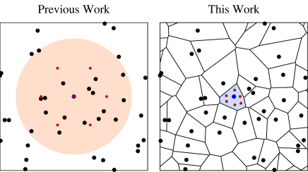
Figure 1: We compare the isotropic particle splitting scheme (left) and our new scheme based on the Voronoi diagram (right) in two dimension. In the left panel, the central particle (blue point) is split to seven daughter particles (red points) distributed within the smoothing length of the parent particle (orange-shaded region). In the right panel, the daughter particles are placed within the Voronoi cell of the central particle (blue-shaded region).

2 Splitting Method

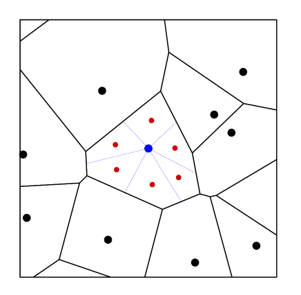
Figure 2: Two-dimensional illustration of the coordinates of daughter particles (red dots) around the parent particle (blue dot). A daughter is on the center of mass of a subcell defined by a blue-dotted line which connects the parent and the middle point of each Voronoi edge. The plot is a zoom-in to the central portion of the right panel in Figure 1.

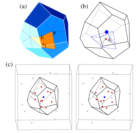
Figure 3: Top panels (a) and (b): Configuration of a subcell (orange region and blue-dotted lines) and the position of a daughter particle (red dot) around a parent particle (blue dot). Bottom panel (c): Stereograph of the daughter particles (red dots) replacing the central parent particle (blue dot) by our splitting method. Black solid lines indicate the Voronoi edges and grey dots indicate the neighbor particles around the target parent particle.

We construct the Voronoi diagram as follows. In our scheme, the Voronoi cell for each particle is obtained. We set a cube of size $2l_{\rm cube}$ centered at a target parent particle as a first trial Voronoi cell. The cube is then cut by a perpendicular bisector of a line segment which connects the central particle and each particle in the cube. After the cube is cut by all the bisectors, we obtain the Voronoi cell. Let us call this procedure the facet-cut algorithm. Initially the cube size is set as $l_{\rm cube}=h_{\rm parent}$. Particles outside the initial cube but closer to the central particle than $2l_{\max}$ can define the final shape of the Voronoi cell, where $l_{\max}$ is the maximal distance between the central particle and the vertices of the Voronoi cell. If $l_{\max}$ is larger than $l_{\rm cube}/2$, we enlarge the initial cube and repeat the facet-cut algorithm. This algorithm scales as ${\cal O}(N_{\rm sp}\log N_{\rm sp})$–${\cal O}(N_{\rm sp}^{2})$ for the number of split particles $N_{\rm sp}$, with a weak dependence on the distribution of the particles.

There are various possibilities to determine the coordinates and mass of the daughter particles. Basically, the daughter particles of a single parent are desired to be well separated to each other and to have a nearly equal mass. Figure 2 shows an example set of the daughter particles. We split the Voronoi cell of the central parent particle (blue dot) into small subcells defined by the blue dotted lines. A subcell corresponds to each Voronoi vertex. A daughter is then placed at the center of mass of each subcell. In this way, we can realize an approximately equal mass distribution of the daughter particles.

We extend the above procedure to three-dimensional cases. Figure 3 illustrates our procedure. We begin with the configuration given in the panel (a). We first draw a boundaries of subcells on each Voronoi plane by the blue dotted line between the two points $P$ and $E$, where $P$ is the center of mass of the Voronoi plane, and $E$ is the middle point of the Voronoi edge. We then define the base planes of the subcell corresponding to a vertex $v_{i}$ as the orange-colored region. The whole shape of the subcell is defined as the polyhedron surrounded by the blue dotted lines in the panel (b). The polyhedron consists of the base planes with the thick blue-dotted lines in the panel (b), which is the same as the orange region in the panel (a), and the target parent particle (blue dot in the panel (b)). Next, we merge the subcells whose corresponding vertices are connected by the shortest edges. We perform this merging procedure in order not to have daughter particles significantly close to each other. A Voronoi cell in 3D typically has 20–30 vertices. If the number of the Voronoi vertices is more than ten, we repeatedly merge the closest subcells until the total number is reduced to ten. At this point we obtain a nearly uniform distribution of the daughters. We choose the threshold number $N_{\rm th}=10$, because we do not want to have a huge mass difference between the parent and the daughters. Refinement by a factor of ten is a reasonable choice. We have actually performed an additional simulation in which subcells are not merged and have confirmed that the results are not significantly affected by the threshold number. We finally put a daughter particle at the center of mass of each (merged) subcell as shown by the red dot in the panel (b).

The bottom panel in Figure 3 is a stereogram showing the distribution of the ten daughters (red dots) generated around the parent (blue dot). We equally divide the mass of the parent particle into $m_{\rm daughter}=m_{\rm parent}/10$. We give the daughters the same temperature as that of the parent. The velocity of the parent particle is simply assigned to the daughters so that the linear momentum and kinetic energy are strictly conserved. The daughters are given half the integration timestep of their parent as a temporal value after splitting, but the individual integration timestep is recalculated for the new set of particles in the next timestep.

3 TEST SIMULATIONS

We perform three test simulations to examine the splitting methods of the previous study (SPHERE) and ours (VORO). We are particularly interested in how the new density field after splitting differs from the original density field represented by the parent particles. In the following tests, we use the SPH code gadget-2 (Springel, 2005) supplemented with the parallelized algorithms of the Voronoi tessellation and the particle splitting. All the control parameters are set to be the default values of gadget-2.0.7. To determine the SPH kernel size, we fix the number of the neighbor particles to $N_{\rm ngb}=50\pm 1$. The densities of SPH particles are calculated in the standard manner using the cubic spline kernel.

3.1 Random and Uniform Particle Distributions

Table 1: Density deviations just after the particle splitting for random particle distributions

run	$\rho_{\max}$	$\rho_{\min}$	$\bar{\rho}$	$\sigma_{\rho}$
UNIF-HALF-SPHERE	3.76	0.49	1.12	0.248
UNIF-HALF-VORO	1.65	0.63	1.04	0.141
UNIF-ALL-SPHERE	4.03	0.72	1.17	0.223
UNIF-ALL-VORO	1.89	0.71	1.07	0.149

We first run simple simulations of an isothermal gas without gravity. We distribute $16^{3}$ SPH particles randomly in the cubic box of $x\in[0,1)$, $y\in[0,1)$, and $z\in[0,1)$ and adopt the periodic boundary conditions. The total mass of the particles is 1 and thus the mean volume-averaged density is $\bar{\rho}_{\rm ini}=1$ in the code unit. The initial particle mass is $m_{\rm p,ini}=1/16^{3}$. We set the isothermal sound speed $c_{T}$ such that the sound crossing time is equal to the unit time. Since the typical length scale of the density fluctuation resulting from the random noise is comparable to the smoothing length of the particles, we define the characteristic sound crossing time as $t_{\rm sc}=\bar{h}_{\rm ini}/c_{T}$, where $\bar{h}_{\rm ini}=\left(3N_{\rm ngb}m_{\rm p,ini}/4\pi\bar{\rho}_{\rm ini}\right)^{1/3}$ is the initial mean smoothing length. We first run a simulation to $t=10$ without particle splitting to reduce the random noise by the gas pressure. At the time, the deviation of the density $\sigma_{\rho}$ is reduced down to 0.0026. The maximal and minimal densities are found to be $(\rho_{\max},\rho_{\min})=(1.08,0.92)$. We call the set of the runs UNIF.

We then split half of the particles in $x\in[0,0.5)$ for run HALF and the all particles for run ALL. Each set is performed with the two splitting methods of SPHERE and VORO. After particle splitting, the root-mean-square of the density $\sigma_{\rho}$ suddenly increases; the maximal density increases and also the minimal density decreases. Note that the particle-averaged density fluctuates around unity after perturbed by the particle splitting. The density deviation eventually approaches to zero and the minimal and maximal densities approach to the mean density because of the gas pressure. We summarize the results in Table 1. The second to fifth columns show the maximal, minimal, average, and root-mean-square of the density just after the particle splitting, respectively.

For the run HALF, the density deviation from the initial value is smaller with VORO than with SPHERE. The maximal and minimal densities just after the splitting change from $(\rho_{\max},\rho_{\min})=(3.76,0.49)$ to $(1.65,0.63)$, with the latter being closer to 1. The density deviation is also reduced from 0.25 to 0.14. The average density is larger than the original density by 12 % for SPHERE, while 4 % for VORO. In the region $x\in(0.1,0.4)$ populated with the fine particles, the density is overestimated at most by a factor of 4 and underestimated by a factor of 0.3 for SPHERE, whereas the density is overestimated by a factor of 0.6 and underestimated by a factor of 0.4 for VORO. At the boundary of the split and un-split particles, the density of the coarse particles is overestimated by a factor of 2.5 and underestimated by a factor of 0.5 for SPHERE, while the density deviates by a factor of 0.3 for VORO. At the time $t=20$, when we stop the simulations, the density difference still remains at the boundary. The maximal and minimal densities are 0.3 and 0.2 for SPHERE and VORO, respectively. Because the particles with different masses are mixed near the boundary, the local density does not quickly converge to the mean value. In practical gas collapse simulations, however, the densest cloud core shrinks more rapidly than the boundaries of fine and coarse particles. Thus the remaining density perturbation on the boundaries would have little effect on the central regions.

For the run ALL, the original density field is well preserved by our splitting method. The maximal density is 1.89 for VORO, which is by a factor of two better than SPHERE. Although the density is slightly more underestimated for VORO. the overestimation of the average density is improved from 17 % to only 7 %, and the root-mean-square of the density is reduced from 0.22 to 0.15. As we have seen in Section 1, the density is overestimated for a particle that is placed significantly close to one of the neighbor particles. This happens with the SPHERE configuration because it involves randomization of the orientation of the daughter particle distribution. With VORO, such an unfortunate case with significant density overestimation does not occur because the coordinates of the daughters are uniquely determined with the separation of any two daughters being a fraction of the distance of their parents. We continue the run and find that another $4.6$ sound-crossing time is required for the density deviation to recover to the initial value 0.026 for both SPHERE and VORO.

3.2 Particle Distribution with Density Gradient

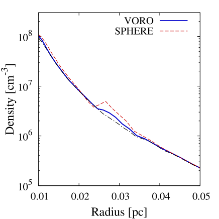
Figure 4: Density profile as a function of the radius for our test GRAD. The black dot-dashed curve shows the density profile before the particle splitting. The solid and dashed lines show the density profiles just after the particle splitting with the methods of the previous (red dashed) and this (blue solid) works, respectively.

It is important to test our method in the case with a steep density gradient. If the length scale of a density fluctuation $l_{\rho}=\rho/|d\rho/dr|$ is smaller than $h_{\rm parent}\sim(N_{\rm ngb}m_{\rm p}/\rho)^{1/3}$, the structure with length scales $\lesssim h_{\rm parent}$ would be smoothed out with the previous splitting method. On the other hand, with our method, the length scale over which the daughter particles are distributed is comparable to the inter-particle distance $\lambda_{\rm p}\sim(m_{\rm p}/\rho)^{1/3}$ before split. Thus, the length over which the density profile is affected is expected to be much smaller. To illustrate this, let us consider a spherical cloud with a large density gradient $\rho\propto r^{-4}$, corresponding to small $l_{\rho}$. Such structure can be seen on the edge of the disk in rotating isothermal clouds (Section 3.3), and also in a volume within a primordial gas cloud where the transition lines of HD molecules becomes optically thick (see Section 4). We call this test GRAD.

We realize the desired density profile with $\rho\propto r^{-4}$ by perturbing particles that are homogeneously distributed initially. The black dot-dashed curve in Figure 4 shows the generated density profile. The sound speed of the cloud is $c_{s}=1\ {\rm km\ s^{-1}}$, corresponding to $T=100$ K, actually being close to the primordial gas cloud temperature. Then, we split the particles with densities $n_{{\rm H}}>3\times 10^{6}\ {\rm cm^{-3}}$. At the density, the length scale of the density variation is $l_{\rho}=r/4=0.006$ pc. The red dashed curves and blue solid curves in Figure 4 show the density profiles just after the particle splitting of the previous and our works. The density profile is flattened at $r=0.03$ pc over the length scale $\sim h_{\rm parent}=0.01$ pc for SPHERE, while we find only a small bump with $\sim\lambda_{\rm p}\sim 0.004$ pc with our method. The daughter particles located within the inter-particle distance of their parent can preserve the density structure before splitting. Note that we consider a spherical cloud in this test. For a cloud with anisotropic density structures, distributing the daughters isotropically results in smoothing the original density structure. The artificial smoothing is mitigated with our method, as we will see in the case of a primordial cloud in Section 4.

3.3 Bodenheimer test

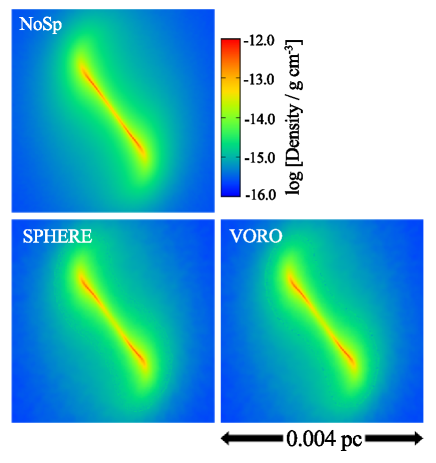
Figure 5: Density slice on the equatorial plane for the Bodenheimer test simulations without particle splitting (NoSp: top) and with the particle splitting of the previous work (SPHERE: bottom left) and the present work (VORO: bottom right) when the maximal density is $\sim 5\times 10^{12}\ {\rm cm^{-3}}$.

Figure 6: Radial profile of the density for Bodenheimer test simulations without the particle splitting (NoSp: black dot-dashed) and with the particle splitting of the previous work (SPHERE: red dashed) and the present work (VORO: blue solid). Note that the red and blue curves closely lie on each other in the plot.

Table 2: Density deviations for BB79 tests

run	$N_{{\rm p,ini}}$	$N_{{\rm p,fin}}$	$\frac{\rho_{\max}}{\bar{\rho}}$	$\frac{\rho_{\min}}{\bar{\rho}}$	$\frac{\sigma_{\rho}}{\bar{\rho}}$
BB79-NoSp	113,098,912
BB79-SPHERE	4,188,896	15,925,664	5.54	0.41	0.33
BB79-VORO	4,188,896	12,805,187	2.22	0.62	0.15

Next, we perform a well-known test introduced by Boss & Bodenheimer (1979) (BB79). We follow gravitational collapse of an isothermal cloud with and without the particle splitting. The cloud mass is $M_{\rm ini}=1\ {\rm M_{\odot}}$ and its radius is $R_{\rm ini}=0.02$ pc initially. The isothermal sound speed of the gas is $c_{T}=0.17\ {\rm km\ s^{-1}}$. The ratio of the thermal energy to the gravitational energy is $\alpha_{\rm ini}=5c_{T}^{2}R_{\rm ini}/2GM_{\rm ini}=0.32$. We set the initial angular velocity $\Omega_{\rm ini}=7.2\times 10^{-13}\ {\rm s^{-1}}$ and then the ratio of the rotational energy to the gravitational energy is $\beta_{\rm ini}=\Omega_{\rm ini}^{2}R_{\rm ini}^{3}/3GM_{\rm ini}=0.28$. The amplitude of $m=2$ perturbation is $A_{m=2,{\rm ini}}=0.1$. The particles are distributed initially on a regular grid, and the particle mass is modulated as $m_{{\rm p,ini}}=\bar{m}_{{\rm p,ini}}(1+A_{m=2,{\rm ini}}\cos 2\phi/2)$, where $\bar{m}_{{\rm p,ini}}$ is the initial average particle mass, and $\phi$ is the azimuthal angle of the particles.

The semi-analytic approaches by Tsuribe & Inutsuka (1999b) show that, in the cloud with $(\alpha,\beta)=(0.32,0.28)$, the non-axisymmetric structure of the gas evolves, and the fragmentation property depends on the initial amplitude of the perturbation. Tsuribe & Inutsuka (1999a) perform the three-dimensional simulations and conclude that such cloud fragments if the initial amplitude is larger than 0.15. In the BB79 test, we run simulations with the minimal mass resolutions ${\cal R}_{\rm cr}=1$, 10, and 100. For ${\cal R}_{\rm cr}=1$ and 10, artificial fragmentation occurs for the lack of the resolution as suggested by Truelove et al. (1997). We here show the results for ${\cal R}_{\rm cr}=100$.

We perform three runs and compare them. In the run NoSp, we distribute a very large number of particles ($N_{\rm p}\sim 10^{8}$) to satisfy the Jeans criterion ${\cal R}\equiv M_{\rm Jeans}/M_{\rm min}\gtrsim 100$ until the gas density reaches $5\times 10^{-12}\ {\rm g\ cm^{-3}}$, where the gas would become optically thick. In the runs SPHERE and VORO, we initially distribute $N_{\rm p,ini}\sim 4\times 10^{6}$ particles. When particles meet the splitting criteria, i.e., violating the Jeans condition, they are split one by one in the course of the simulations.

Figure 5 shows the density slice of the clouds for NoSp (top), SPHERE (bottom left), and VORO (bottom right) at the maximal density $\rho_{\rm cen}=5\times 10^{-12}\ {\rm g\ cm^{-3}}$. The stretched thin filament does not fragment in all the three runs up to the last output time as reported by Tsuribe & Inutsuka (1999b). Figure 6 shows the evolution of the density profiles as a function of the distance from the densest part of one end of the filament. The overall structure of the filament remains essentially the same among the three runs. We conclude that the resolution ${\cal R}_{\rm cr}=100$ is sufficient when we consider collapse and fragmentation of the cloud. The number of particles is $N_{\rm p,fin}\sim 10^{7}$ for SPHERE and VORO when we terminate the simulations at $\rho_{\rm cen}=5\times 10^{-12}\ {\rm g\ cm^{-3}}$, which is by an order of magnitude less than NoSp. This means that the computational cost is well reduced by the splitting technique although the final snapshots are similar to the one for NoSp.

Let us compare the two runs SPHERE and VORO in detail. We follow the density deviations of the 1000 particles that are split first. The results are summarized in Table 2. The particles are split for the first time when $\rho=3\times 10^{-15}\ {\rm g\ cm^{-3}}$. Just before the splitting, the maximal and minimal densities relative to the mean density of the 1000 particles are 1.08 and 0.85, respectively, and the deviation of the density is 0.037. Just after the 1000 particles are split, the density deviation marks the maximum. In the SPHERE and VORO runs, the maximal and minimal densities just after the particle splitting are $(\rho_{\max}/\bar{\rho},\rho_{\min}/\bar{\rho})=(5.54,0.41)$ and $(2.22,0.62)$, respectively. The maximal deviations of the density from the original value 1 are reduced more than by a factor of two by our splitting method. The density deviation relative to the mean density just after the splitting also decreases from 0.33 (SPHERE) to 0.15 (VORO), approaching to the initial value of 0.037. The result shows that, also in the practical collapse simulation, the daughter particles distributed in a Voronoi cell of each split particle are not close to other neighbor particles, and their density is not significantly overestimated, while this happens with the conventional splitting method.

In this BB79 test, the density structure is not very different between SPHERE and VORO, showing an interesting contrast to our test GRAD that is more relevant to a primordial warm gas (see Section 3.2). In the cold gas with small $c_{T}$ in BB79, the smoothing length $h_{\rm parent}\sim c_{T}{\cal R}_{\rm cr}^{-1/3}(G\rho)^{-1/2}$ is smaller than the length scale $l_{\rho}$ all over the region if the critical condition is set as ${\cal R}_{\rm cr}=100$. On the iso-density surface of $\rho=5\times 10^{-13}\ {\rm g\ cm^{-3}}$, where the second particle splitting occurs, $l_{\rho}$ is smallest, $4\times 10^{-6}\ {\rm pc}$, at the edge of the iso-density filament. The smoothing length in the region is $h_{\rm parent}=3\times 10^{-6}\ {\rm pc}$. SPH particles which satisfy the Jeans criterion ${\cal R}_{\rm cr}=100$ can resolve the density structure when the gas is sufficiently cold ($c_{T}\sim 0.1\ {\rm km\ s^{-1}}$). This is, however, not in the case of the primordial warm gas as we revisit with detailed discussion later in Section 4.

4 Collapse simulations of primordial gas cloud

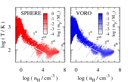
Figure 7: Distribution of the particles on the thermodynamic phase plane in the simulations of primordial gas cloud formaton, when the central density $n_{\rm H,cen}=10^{7}\ {\rm cm^{-3}}$. The color indicates the mass-weighted number of the particles. Left and right panel show the result with the particle splitting of SPHERE and VORO, respectively. The dotted lines attached to the orders ‘$n$th’ indicate the density and temperature where the particles are split for the $n$th time. The SPH particles in the region below the white diagonal line have temperatures that are underestimated due to the particle spitting.

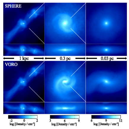
Figure 8: Projected density distribution of the primordial clouds from the face-on and edge-on views of the disk methods of SPHERE (top) and VORO (bottom) when the central density is $10^{12}\ {\rm cm^{-3}}$.

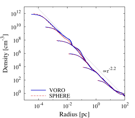
Figure 9: Radial density profile of the primordial cloud with the particle splitting methods SPHERE (red dashed) and VORO (blue solid). We also plot the grey dotted line $\propto r^{-2.2}$ which a primordial gas cloud tends to be along.

Finally, we apply our splitting method to a more realistic calculation of the collapse of a primordial minihalo. We isolate the spherical region with length $\sim 1$ kpc centered at one of the minihalos formed at the redshift $z=15$ in the cosmological simulation of Hirano et al. (2014). The mass of the halo is $M_{h}=4.8\times 10^{5}\ {\rm M_{\odot}}$. The halo is categorized to a subclass of the primordial minihalos which hosts less massive stars ($10$–$100\ {\rm M_{\odot}}$) because of the efficient cooling by HD molecules. The chemical reaction rates and radiative cooling rates are taken from Chiaki et al. (2015) for a primordial composition. We reduce the cooling rates of emission lines by the Sobolev length method in the optically thick regime as in Hirano & Yoshida (2013). The splitting methods of the privious work (SPHERE) and this work (VORO) are employed for the gas particles. The number of neighbor particles is restricted to be $N_{\rm ngb}=64\pm 8$, and the criterion for the particle splitting is ${\cal R}_{\rm cr}=1000$ as set by Hirano et al. (2014). The central particles are already once split by SPHERE splitting when the zoomed initial conditions are generated. The initial particle mass is $m_{\rm SPH}^{(1)}=5/13\ {\rm M_{\odot}}$. The number of gas particles is initially 169,511. When the central density reaches $n_{{\rm H}}=10^{12}\ {\rm cm^{-3}}$, the particles have been split at most five times and the number of split particles increases up to 314,867 for SPHERE and 318,148 for VORO.

Figure 7 shows that distribution of the gas particles in the density-temperature plane. We use the snapshot when the central density $n_{\rm H,cen}=10^{7}\ {\rm cm^{-3}}$. Note that HD cooling operates at the densities $n_{{\rm H}}\gtrsim 10^{3}{\rm cm^{-3}}$, where a disk structure is formed with noticeable spiral arms. The particles are split at the densities and temperatures indicated by the dotted lines in Figure 7. The index ‘$n$th’ attached to the dotted lines indicates the criterion for the $n$th particle splitting: $M_{\rm Jeans}={\cal R}_{\rm cr}N_{\rm ngb}(m_{\rm SPH}^{(1)}/13^{n-1})$ and ${\cal R}_{\rm cr}N_{\rm ngb}(m_{\rm SPH}^{(1)}/10^{n-1})$ for SPHERE and VORO, respectively. We see that the temperature significantly fluctuates along the adiabatic line $T\propto n_{{\rm H}}^{2/3}$ from the splitting points for SPHERE. Since the gas cooling and heating do not work promptly within a short timestep, the temperatures of daughters deviate along the adiabatic line when their densities are perturbed from the parent’s density one timestep after splitting. Thus the temperature deviation almost directly reflects the density perturbation induced by the particle splitting. The white lines in Figure 7 indicate the expected trajectories, i.e., the gas particles having the lowest temperature at each density would evolve roughly on the white line without the particle splitting. The figure shows that our splitting method slightly improves the temperature deviation from the splitting point. The distributions of particles on the density-temperature planes are not significantly different for two splitting methods SPHERE and VORO.

We find that substantial differences are caused in the global structure by the two different splitting methods. Figure 8 shows the snapshots of the gas cloud at the central density $n_{\rm H,cen}=10^{12}\ {\rm cm^{-3}}$. Comparing the middle panels, we find that the spiral arms have more developed in VORO than in SPHERE. This is related to the associated smoothing and isotropization after split, as we discussed in Section 3.2. At densities $n_{{\rm H}}\sim 10^{6}$–$10^{7}\ {\rm cm^{-3}}$, where the emission lines from HD molecules becomes optically thick, $l_{\rho}$ is reduced to $\sim 0.01$ pc because of the rapidly increasing pressure. The length at which the daughter particles are distributed is $\sim h_{\rm parent}\sim(N_{\rm ngb}m_{\rm p}/\rho)^{1/3}\simeq 0.01$ pc in run SPHERE and $\sim\lambda_{\rho}\sim(m_{\rm p}/\rho)^{1/3}\simeq 0.004$ pc in run VORO. Even for the same Jeans criterion, our splitting method allows to make the resolution of daughter particles effectively higher than in SPHERE by a factor of $\sim h_{\rm parent}/\lambda_{\rm p}\sim N_{\rm ngb}^{1/3}$.

Figure 9 shows the radial density profile and its evolution. Our splitting method maintain the steep density profile at the densities $n_{{\rm H}}\sim 10^{6}\ {\rm cm^{-3}}$ where the emission lines of HD molecules are optically thick, and at $\sim 10^{8}\ {\rm cm^{-3}}$ where the gas heating by H₂ molecular formation via the three-body reactions is dominant. The right panels of Figure 8 show that the bar-like structure has developed in VORO while the central region appears smooth and spherical in SPHERE. Clearly, details of splitting method affect the evolution of the global structure such as spiral arms and also the fragmentation of the cloud core.

We suspect from the tests GRAD and BB79 that the anisotropic density structure in the primordial collapsing gas is smoothed by the isotropic distribution of daughter particles. In a warm gas cloud with large $c_{T}$ such as a primordial gas cloud, the length $l_{\rho}$ can not be resolved by $h_{\rm parent}\propto c_{T}{\cal R}_{\rm cr}^{-1/3}(G\rho)^{-1/2}$ even though the Jeans criterion with ${\cal R}_{\rm cr}=1000$ is satisfied. To avoid the isotropic diffusion of density structures in a warm gas where $c_{T}\gtrsim 1\ {\rm km\ s^{-1}}$, we should impose a severer Jeans criterion with larger resolution threshold ${\cal R}_{\rm cr}$ such that $l_{\rho}$ can be resolved by the coarse particles with the conventional splitting method (see Section 5). Our method overcomes this problem by distributing the fine particles within an inter-particle distance from the parent, which shortens the effective resolution of the gas particles. Therefore, it is not necessary to have severer criteria for splitting than the Jeans criterion.

5 DISCUSSION

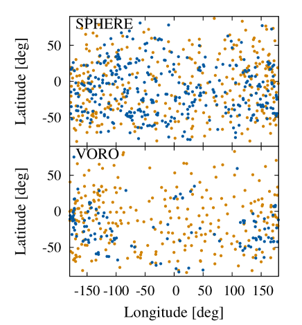
Figure 10: Distribution of the SPH particles above (orange) and below (blue) the white line in Figure 7 on the iso-density sphere with $n_{{\rm H}}=10^{3}\ {\rm cm^{-3}}$ for the splitting methods of the previous (top) and this work (bottom).

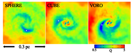
Figure 11: Distribution of the Toomre $Q$ parameter in the disk from the face-on view for runs SPHERE (left), CUBE (middle) and VORO (right) in the same region as the middle panels of Figure 8. The $Q$ parameter is smallest at the white squares in the spiral arms.

We have developed a novel method for particle splitting in SPH simulations based on the Voronoi diagram (VORO). Our series of tests show that the new method preserves well the original density structure before splitting, while achieving an effectively high resolution. The density perturbations induced by the splitting are reduced by a factor of two compared with the conventional splitting method (SPHERE). We have found that similar improvements are achieved by another particle splitting method of MES06 (CUBE hereafter), where daughters are distributed within a distance $h_{\rm parent}/8$ ($\simeq\lambda_{\rm p}/4$) from their parent. In the test GRAD, the density profile is similar to VORO. Only the slight bump appears at the splitting point over the length scale $\sim\lambda_{\rm p}$. In the test BB79, the morphology and the density profile is similar to runs SPHERE and VORO. The density deviation just after the splitting is better than VORO. The maximal and minimal densities relative to the average density of 1000 particles first split are 1.91 and 0.68, respectively. The root-mean-square of the density is 1.03.

In the case of a contracting primordial gas cloud, where the gas no longer evolves isothermally, the temperature deviates along with the density perturbation generated by the particle splitting as Figure 7 shows. Some particles are overcooled and might trigger the artificial fragmentation by their small pressure, but this would not be in the case. Figure 10 shows the spatial distribution of the SPH particles on the iso-density surface with $n_{{\rm H}}=10^{3}\ {\rm cm^{-3}}$. We divide the gas particles into hot (orange) and cool (blue) components respectively above and under the white line in Figure 7. The blue dots indicate the overcooled gas. If the overcooled gas particles cluster, they might trigger the fragmentation by their small pressure. However, the cool gas particles apparently scatter in all directions for SPHERE (upper panel). For VORO, although the cool component appears to cluster at longitude $180^{\circ}$, where a spiral arm lies, the hot gas particles are also in the arm region and would prevent the collapse of the cool component. The local perturbations of temperature and density triggered by the particle splitting would not affect the gas fragmentation irrespective of the splitting methods.

On the other hand, the global density structure such as spiral arms and bars can affect the gravitational stability of the gas. As seen in Figure 8, the high-density region remains strongly elongated in VORO run. Although the long-time evolution of the spiral arms is not followed in our simulations, we can derive a reasonable estimate on whether or not the disk is stable by calculating the Toomre $Q$ parameter $Q=2\Omega c_{T}/\pi G\Sigma$, where $\Sigma$ is the column density in each part on the disk. Figure 11 shows the distribution of $Q$ parameter. Clearly, the value of $Q$ is small along the spiral arms and is the smallest at the point indicated by the white square in each panel: $Q_{\min}=0.59$ for SPHERE and 0.41 for VORO. We have also performed the collapse simulation with the splitting method CUBE. The distribution of $Q$ parameter is shown in the middle panel of Figure 11. The elongation of the central core is slightly smaller than our method VORO. The inner structure of the spiral arms is resolved as well as VORO, but the density structure appears slightly more diffuse. This is likely because of the nature of the method of CUBE, where the daughter particles are distributed on the vertices of the cube around a parent, and the original density structure formed by parent particles are slightly smoothed in the directions both perpendicular and parallel to the disk. The column density in the spiral arms for the run CUBE is less than VORO, and the resulting minimal $Q$ parameter is 0.58. The linear analysis of the ring-mode instabilities by Takahashi (2015) suggests that spiral arms with $Q\lesssim 1/\pi$ is dynamically unstable and likely produce fragments. We can say that the spiral arms are marginally stable against fragmentation in the both runs at the time of the snapshot. Still, the difference in the global structure of the protostellar disk affects the evolution of the central protostar in a complicated manner (see e.g. Greif et al., 2012; Vorobyov et al., 2013). It is important to fully resolve the disk structure over a long time.

Our test simulations suggest that the mass resolution with VORO is effectively higher than with SPHERE by a factor of $\sim h_{\rm parent}/\lambda_{\rm p}\sim N_{\rm ngb}^{1/3}$. We find that small-scale anisotropic structures are smoothed out when the particles are split in the region with steep density gradient with insufficient resolution with SPHERE method. To avoid the artificial mixing, we suggest to impose an additional criterion than the Jeans criterion for splitting with the conventional splitting method with spherical distribution of daughters: the length scale of the density fluctuation $l_{\rho}$ should be sufficiently resolved by the local SPH smoothing length. To confirm this, we have performed another simulation with SPHERE splitting with a substantially higher resolution of ${\cal R}_{\rm cr}=4000$. The high-resolution run indeed shows an elongated cloud and apparent spiral arms, similarly to those found in the VORO run. We emphasize that our splitting method performs only with the modest Jeans criterion, because the distribution of daughters traces the original anisotropic density structure before splitting. The method saves computational cost by effectively reducing the number of particles necessary to resolve the cloud structures.

It is actually costly to construct the Voronoi diagrams with the current algorithm. In the simulations with ${\cal R}_{\rm cr}=1000$, the computational time until the density of the cloud center reaches $n_{\rm H,cen}=1\times 10^{12}\ {\rm cm^{-3}}$ is 48,315 (SPHERE) and 81,320 (VORO) seconds using 128 cores. The Voronoi tessellation accounts for about a half of the total computational time. However, in the simulation of SPHERE with ${\cal R}_{\rm cr}=4000$, where the bar-like structure is seen also with the conventional splitting method, the computational time is 323,309 seconds, exceeding the time for VORO with ${\cal R}_{\rm cr}=1000$. Clearly, the formation of small-scale structrue such as the bar-like structure is accurately followed with smaller computational time with our splitting method. We can further save the computational cost for generation of the Voronoi tessellation by introducing the incremental construction algorithm scaling as ${\cal O}(N\log N)$ (Sugihara & Iri, 1994) . In a forthcoming paper, we present an efficient scheme to parallelize the algorithm that scales as ${\cal O}(N)$ (Chiaki, Yoshikawa & Yoshida in prep.).

We note that there have been some simplifications adopted in our method. First, we place the daughter particles at the center of the mass of the subcells as shown in Figure 3. Another promising choice might be to place daughters such that the original Voronoi planes between the parent and the neighboring particles are not affected even after the splitting. Second, we still follow the traditional SPH scheme to solve the equation of motion. Saitoh & Makino (2013) point out that the traditional SPH scheme causes asymmetric errors of density and pressure estimations at boundaries between the two phases with different densities. The density and pressure errors obviously affect the fluid motion. We find that, in the case of our particle splitting, the pressure perturbation at the boundary between the fine and coarse regions nearly cancel out and thus spurious force is not induced. Third, the distribution of the parent particles has intrinsic noise due to its discrete nature. Then unphysical anisotropic shapes of the Voronoi cells might generate and even promote density perturbations. We could regulate the shapes of the Voronoi cells by Lloyd’s algorithm (Lloyd, 1982), which is expected to yield accurate density estimates. Finally, we adopt the cubic spline kernel to estimate the density as in the standard SPH. The choice of other kernel functions and the number of the neighbor particles would affect the accuracy of the density reconstruction. Overall, we have shown that our splitting method based on the Voronoi diagram improves the preservation of the density and the morphology of gravitationally contracting clouds even with the minimal implementation, but further studies are certainly warranted to optimize the choice and the implementation of each part of the splitting scheme.

The splitting method can be applied not only to simulations of star forming clouds but also to other astrophysical problems. For example, in the downstream of the cooling shocks, the density rapidly increases by three orders of magnitude (Chiaki et al., 2013). The density structure is highly anisotropic around the shock front by hydrodynamic instabilities. The dense shocked region can be fully resolved by our splitting method while maintaining the fine structure. We can also perform de-refinement of the particles as the converse operation of the particle splitting. The particles to be merged can be uniquely identified once we define the Voronoi diagram. An example implemented in a moving-mesh code is found in arepo (Springel, 2010). The de-refinement can also be applied to the problem of an interstellar shock, where the density of fluid elements decreases after passing through the shocked region. In such cases, de-refinement of particles behind the shock will significantly save the number of particles and the overall computational time. We continue developing the de-refinement techniques based on the Voronoi diagrams. Our method of particle spitting presented here and de-refinement technique can be applied to particle-based simulations of various problems as elaborated schemes both to preserve complex density structures and to save the computational cost.

References

- Boss & Bodenheimer (1979) Boss, A. P., & Bodenheimer, P. 1979, ApJ, 234, 289
- Bromm & Loeb (2003) Bromm, V., & Loeb, A. 2003, ApJ, 596, 34
- Vorobyov et al. (2013) Vorobyov, E. I., DeSouza, A. L., & Basu, S. 2013, ApJ, 768, 131
- Chiaki et al. (2013) Chiaki, G., Yoshida, N., & Kitayama, T. 2013, ApJ, 762, 50
- Chiaki et al. (2015) Chiaki, G., Marassi, S., Nozawa, T., et al. 2015, MNRAS, 446, 2659
- Dotti et al. (2007) Dotti, M., Colpi, M., Haardt, F., & Mayer, L. 2007, MNRAS, 379, 956
- Greif et al. (2012) Greif, T. H., Bromm, V., Clark, P. C., et al. 2012, MNRAS, 424, 399
- Hirano et al. (2014) Hirano, S., Hosokawa, T., Yoshida, N., et al. 2014, ApJ, 781, 60
- Hirano & Yoshida (2013) Hirano, S., & Yoshida, N. 2013, ApJ, 763, 52
- Hopkins (2014) Hopkins, P. F. 2014, arXiv:1409.7395
- Kitsionas & Whitworth (2002) Kitsionas, S., & Whitworth, A. P. 2002, MNRAS, 330, 129
- Lloyd (1982) Lloyd, S. 1982, IEEE Trans. Inform. Theory, 28, 129
- Martel et al. (2006) Martel, H., Evans, N. J., II, & Shapiro, P. R. 2006, ApJS, 163, 122
- Mayer et al. (2010) Mayer, L., Kazantzidis, S., Escala, A., & Callegari, S. 2010, Nature, 466, 1082
- Saitoh & Makino (2013) Saitoh, T. R., & Makino, J. 2013, ApJ, 768, 44
- Springel (2005) Springel, V. 2005, MNRAS, 364, 1105
- Springel (2010) Springel, V. 2010, MNRAS, 401, 791
- Sugihara & Iri (1994) Sugihara, K., & Iri, M. 1994, Int. J. Comput. Geom. Appl. 04, 179
- Takahashi (2015) Takahashi, S. 2015, Ph.D. Thesis, Kyoto University
- Truelove et al. (1997) Truelove, J. K., Klein, R. I., McKee, C. F., et al. 1997, ApJ, 489, L179
- Truelove et al. (1998) Truelove, J. K., Klein, R. I., McKee, C. F., et al. 1998, ApJ, 495, 821
- Tsuribe & Inutsuka (1999a) Tsuribe, T., & Inutsuka, S.-i. 1999, ApJ, 523, L155
- Tsuribe & Inutsuka (1999b) Tsuribe, T., & Inutsuka, S.-i. 1999, ApJ, 526, 307
- Turk et al. (2012) Turk, M. J., Oishi, J. S., Abel, T., & Bryan, G. L. 2012, ApJ, 745, 154
- Yoshida et al. (2006) Yoshida, N., Omukai, K., Hernquist, L., & Abel, T. 2006, ApJ, 652, 6