Comparative study of the scalar- and tensor-meson production in the reaction $\gamma\gamma^{*}(Q^{2})\to\eta\pi^{0}$

Abstract

The prediction of the cross section $\sigma(\gamma\gamma^{*}(Q^{2})\to\eta\pi^{0})$ based on the simultaneous description of the Belle data on the $\gamma\gamma\to\eta\pi^{0}$ reaction and the KLOE data on the $\phi\to\eta\pi^{0}\gamma$ decay is presented. The production of the scalar $a_{0}(980)$ and tensor $a_{2}(1320)$ is studied in detail. It is shown that the QCD based asymptotics of the $\gamma^{*}(Q^{2})\gamma\to a_{2}(1320)\to\eta\pi^{0}$ cross section can be reached by the compensation of the contributions of $\rho(770)$ and $\omega(782)$ with the contributions of their radial excitations in $Q^{2}$ channel. At large $Q^{2}$ the $a_{2}(1320)$ contribution is expected to be dominant, while at $Q^{2}=0$ it is similar to the scalars contribution.

I Introduction

Study of the nature of light scalars $a_{0}(980)$ and $f_{0}(980)$, well-established part of the proposed light scalar meson nonet pdg-2014 , is one of the central problems of nonperturbative QCD, it is important for understanding the way chiral symmetry is realized in the low energy region and, consequently, for the understanding of confinement. Many papers have already been devoted to this subject, see, for example, Refs. closeIK ; tornquist ; oller-2012 ; itep ; rosner ; klempt ; volkovRadzhabov ; harada .

Naively one could think that the scalar $a_{0}(980)$ and $f_{0}(980)$ mesons are the $q\bar{q}$ P-wave states with the same quark structure as $a_{2}(1320)$ and $f_{2}(1270)$, respectively. But now there are many indications that the above scalars are four-quark states, see, for example, Refs. jaffe ; joe ; pennington ; fourQuarkGG ; AS88 ; achasov-89 ; achasov-97 ; SNDa0 ; f0exp ; a0f0 ; kloea0 ; our_a0 ; achasov-03 ; achasov-08 ; annsgn2010 ; annsgn2011 and references therein.

One of these indications is the suppression of the $a_{0}(980)$ and $f_{0}(980)$ resonances in the $\gamma\gamma\to\eta\pi^{0}$ and $\gamma\gamma\to\pi\pi$ reactions, respectively, predicted in 1982 fourQuarkGG and confirmed by experiment pdg-2014 , see GGwidths . The elucidation of the mechanisms of the $\sigma(600)$, $f_{0}(980)$, and $a_{0}(980)$ resonance production in the $\gamma\gamma$ collisions confirmed their four-quark structure AS88 ; achasov-08 ; annsgn2010 ; annsgn2011 . Light scalar mesons are produced in $\gamma\gamma$ collisions mainly via rescatterings, that is, via the four-quark transitions. As for the $a_{2}(1320)$ and $f_{2}(1270)$, the well-known $q\bar{q}$ states, they are produced mainly via the two quark transitions (direct couplings with $\gamma\gamma$).

Another argument in favor of the four-quark nature of the $a_{0}(980)$ and $f_{0}(980)$ is the fact that the $\phi(1020)\to a_{0}\gamma$ and $\phi(1020)\to f_{0}\gamma$ decays proceed through the kaon loop: $\phi\to K^{+}K^{-}\to a_{0}\gamma$, $\phi\to K^{+}K^{-}\to f_{0}\gamma$, i.e. via the four-quark transition achasov-89 ; achasov-97 ; a0f0 ; our_a0 ; achasov-03 . The kaon loop model was suggested in Ref. achasov-89 and confirmed by the experiment ten years later SNDa0 ; f0exp ; kloea0 .

Recently the comparative study of the scalar and tensor mesons was proposed in the $e^{+}e^{-}\to\gamma^{*}\to(a_{0}+a_{2})\gamma\to\eta\pi^{0}\gamma$ and $e^{+}e^{-}\to\gamma^{*}\to(f_{0}+f_{2})\gamma\to\pi^{0}\pi^{0}\gamma$ reactions (i.e. in the timelike region of $\gamma^{*}$) agkr-2013 .

In the present study we consider the reaction $\gamma^{*}\gamma\to\pi^{0}\eta$ in the spacelike region of $\gamma^{*}$.

In 2009 Belle Collaboration published high-statistical data on the $\gamma\gamma\to\eta\pi^{0}$ reaction uehara . These data revealed the specific feature of the $\gamma\gamma\to\pi^{0}\eta$ cross section: it turned out sizable in the region between the $a_{0}(980)$ and $a_{2}(1320)$ resonances, that certainly indicates the presence of additional contributions. The experimenters took into account the putative heavy isovector scalar $a_{0}^{\prime}$ with mass about $1.3$ GeV (they called it $a(Y)$) along with $a_{0}(980)$ and $a_{2}(1320)$ together with the polynomial coherent background uehara .

In the theoretical works Refs. annsgn2010 ; annsgn2011 $a_{0}(980)$ is produced mainly by loops, and the Born contribution to $\gamma\gamma\to\eta\pi^{0}$ plays role of coherent background, see Figs. 1, 2. The kaon formfactor $G_{K^{+}}(t,u)$ in loop diagrams $\gamma\gamma\to K^{+}K^{-}\to a_{0}$ was introduced in those papers.

The given paper is the development of the Refs. annsgn2010 ; annsgn2011 . Basing on their theoretical results, we perform new fitting of the Belle data simultaneously with the KLOE data on the $\phi\to\eta\pi^{0}\gamma$ decay. We show that in the kaon loop model of the $\gamma\gamma\to K^{+}K^{-}\to a_{0}$ transition the kaon formfactor $G_{K^{+}}(t,u)$ is not required for good data description, as well as in the $\phi\to K^{+}K^{-}\to a_{0}\gamma\to\eta\pi^{0}\gamma$ decay and $\phi\to K^{+}K^{-}\to f_{0}\gamma\to\pi^{0}\pi^{0}\gamma$ achasov-89 ; achasov-97 ; SNDa0 ; f0exp ; a0f0 ; achasov-03 ; kloea0 ; our_a0 . The obtained $a_{0}(980)$ coupling constants are in good agreement with the four-quark model prediction achasov-89 .

Using results on $\gamma\gamma\to\eta\pi^{0}$ we predict the $\sigma(\gamma^{*}(Q^{2})\gamma\to\eta\pi^{0},s)$, where $s$ is the $\gamma^{*}\gamma$ invariant mass and $Q^{2}$ is the $\gamma^{*}$ virtuality.

The measurement of the cross section $\sigma(\gamma^{*}(Q^{2})\gamma\to\eta\pi^{0},s)$ would allow additional check of the models of the $a_{0}(980)$ structure and our understanding of the mechanism of the reactions $\gamma^{*}\gamma\to\eta\pi^{0}$ as well as $\gamma\gamma\to\eta\pi^{0}$.

The theoretical description of the $\gamma^{*}\gamma\to\eta\pi^{0}$ reaction is in Sec. II. The results on the $\gamma\gamma\to\eta\pi^{0}$ data description are presented in Sec. III. The prediction of the $\sigma(\gamma^{*}(Q^{2})\gamma\to\eta\pi^{0},s)$ is in Sec. IV. It is found that the role of vector excitations ($\rho^{\prime}$, $\omega^{\prime}$, etc.) is crucial for the $a_{2}(1320)$ and $f_{2}(1270)$ production: the QCD based asymptotics of the $\gamma^{*}(Q^{2})\gamma\to a_{2}(1320)\to\eta\pi^{0}$ (or $\gamma^{*}(Q^{2})\gamma\to f_{2}(1270)\to\pi^{0}\pi^{0}$) cross section can be reached only by taking into account cancellation of the contributions of $\rho(770),\omega(782)$ and $\phi(1020)$ in $Q^{2}$ channel with the contributions of their radial excitations. The $a_{2}(1320)$ contribution is expected to be dominant at large $Q^{2}$, while at $Q^{2}=0$ it is similar to the $a_{0}(980)+a_{0}^{\prime}$ contribution. The conclusion is in Sec. V. Some details are provided in Appendices I-III.

Noticed misprints of Refs. annsgn2010 ; annsgn2011 are mentioned in Ref. misprints .

II Theoretical description of the $\gamma^{*}\gamma\to\eta\pi^{0}$ reaction

Figure 1: Diagrammatical representation for the helicity amplitudes $\gamma^{*}\gamma$ $\to$ $\pi^{0}\eta$.

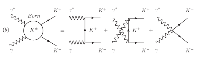
Figure 2: The Born $\rho$, $\omega$, $K^{*}$, $K$ exchange diagrams for $\gamma^{*}\gamma$ $\to$ $\pi^{0}\eta$, $\gamma^{*}\gamma$ $\to$ $\pi^{0}\eta^{\prime}$, and $\gamma^{*}\gamma$ $\to$ $K\bar{K}$.

All formulas for the $\gamma\gamma\to\eta\pi^{0}$ reaction were derived in Refs. annsgn2010 ; annsgn2011 , these results are used to fit the experimental data. In this section we derive formulas for the $\gamma^{*}(q)\gamma(k)\to\eta(q_{1})\pi^{0}(q_{2})$ reaction, $Q^{2}=-q^{2}>0$. The results of Refs. annsgn2010 ; annsgn2011 are reached in the limit $Q^{2}\to 0$.

Most of formulas in this section are modifications of Refs. annsgn2010 ; annsgn2011 results. In all diagrams the vector resonances undergo excitation in the $\gamma^{*}$ line resulting in distinctive factors in the amplitudes.

According to Refs. annsgn2010 ; annsgn2011 , we use a model for the helicity amplitudes $M_{\lambda}$ ($\lambda$ is the difference between photon helicities), taking into account electromagnetic Born contributions from $\rho$, $\omega$, $K^{*}$, $K$ exchanges and strong elastic and inelastic final-state interactions in $\pi^{0}\eta$, $\pi^{0}\eta^{\prime}$, $K^{+}K^{-}$, and $K^{0}\bar{K}^{0}$ channels, as well as the contributions due to the direct interaction of the resonances with photons:

$$M_{0}(\gamma^{*}\gamma\to\pi^{0}\eta;s,Q,\theta)=M^{\mbox{\scriptsize{Born}}\,V}_{0}(\gamma^{*}\gamma\to\pi^{0}\eta;s,Q,\theta)+\widetilde{I}^{V}_{\pi^{0}\eta}(s,Q)\,T_{\pi^{0}\eta\to\pi^{0}\eta}(s)$$

$$+\widetilde{I}^{V}_{\pi^{0}\eta^{\prime}}(s,Q)\,T_{\pi^{0}\eta^{\prime}\to\pi^{0}\eta}(s)+\bigg{(}\widetilde{I}^{K^{*+}}_{K^{+}K^{-}}(s,Q)-\widetilde{I}^{K^{*0}}_{K^{0}\bar{K}^{0}}(s,Q)$$

$$+\widetilde{I}^{K^{+}}_{K^{+}K^{-}}(s,Q)\bigg{)}T_{K^{+}K^{-}\to\pi^{0}\eta}(s)$$

$$+M^{\mbox{\scriptsize{direct}}}_{\mbox{\scriptsize{res}}}(s,Q)+M_{0}(\gamma^{*}\gamma\to a_{2}(1320)\to\pi^{0}\eta;s,Q,\theta),$$ (1)

$$M_{1}(\gamma^{*}\gamma\to\pi^{0}\eta;s,Q,\theta)=M^{\mbox{ \scriptsize{Born}}\,V}_{1}(\gamma^{*}\gamma\to\pi^{0}\eta;s,Q,\theta)$$

$$+M_{1}(\gamma^{*}\gamma\to a_{2}(1320)\to\pi^{0}\eta;s,Q,\theta),$$ (2)

$$M_{2}(\gamma^{*}\gamma\to\pi^{0}\eta;s,Q,\theta)=M^{\mbox{ \scriptsize{Born}}\,V}_{2}(\gamma^{*}\gamma\to\pi^{0}\eta;s,Q,\theta)$$

$$+M_{2}(\gamma^{*}\gamma\to a_{2}(1320)\to\pi^{0}\eta;s,Q,\theta),$$ (3)

the diagrams corresponding to these amplitudes are shown in Figs. 1, 2. Here $\theta$ is the angle between $\pi^{0}$ and $\gamma$ (or $\eta$ and $\gamma^{*}$) momenta in the $\gamma^{*}\gamma$ center-of-mass system.

The kaon loop contribution $\gamma^{*}\gamma\to K^{+}K^{-}\to a_{0}\to\eta\pi^{0}$ (the term $\widetilde{I}^{K^{+}}_{K^{+}K^{-}}(s,Q)T_{K^{+}K^{-}\to\pi^{0}\eta}(s)$) and the $a_{2}$ contribution are the largest ones, but other terms are also essential. $I$-functions are loop integrals, $T$-functions represent rescattering amplitudes (see below).

In the case of real photons $M_{1}(\gamma^{*}\gamma\to\pi^{0}\eta)$ vanishes because of the electromagnetic current conservation. The $M_{0}(\gamma^{*}\gamma\to a_{2}(1320)\to\pi^{0}\eta)$ is small at $Q=0$ according to experiment.

The cross sections $\sigma_{\lambda}\equiv\sigma_{\lambda}(\gamma^{*}\gamma\to\eta\pi^{0},s,Q)$ are related to the amplitudes $M_{\lambda}$ as

$$\sigma_{\lambda}=\frac{\rho_{\pi\eta}(s)}{64\pi s\rho_{\gamma^{*}\gamma}}\int^{0.8}_{-0.8}|M_{\lambda}|^{2}d\cos\theta\,,\hskip 14.22636pt\rho_{\gamma^{*}\gamma}=1+Q^{2}/s\,,$$ (4)

$$\bar{\sigma}_{\lambda}=\frac{1}{2a}\int^{\sqrt{s}+a}_{\sqrt{s}-a}\sigma_{\lambda}(s^{\prime})d\sqrt{s^{\prime}}\,,$$ (5)

and the total cross section $\sigma(\gamma^{*}(Q^{2})\gamma\to\eta\pi^{0},s)=\sigma_{0}+\sigma_{1}+\sigma_{2}$. The limits $|\cos\theta|\leq 0.8$ and bin size $2a=20$ MeV were used in the experiment Ref. uehara , where the data on the sum $\bar{\sigma}_{0}+\bar{\sigma}_{2}$ at $Q=0$ were presented for different values of $\sqrt{s}$ ($\sigma_{1}=\bar{\sigma}_{1}=0$ at $Q=0$).

Let us derive all the terms in Eqs. (1), (2), and (3).

The Born term $M^{\mbox{\scriptsize{Born}}\,V}_{\lambda}$ is caused by equal equalBorn contributions of the $\rho$ and $\omega$ exchange mechanisms AS88 . It is calculated by Vector Dominance Model (VDM), the result is the significant modification of Eqs. (3) and (4) of Ref. annsgn2010 :

$$\mbox{\qquad\ \ \ }M^{\mbox{\scriptsize{Born}}\,V}_{0}(\gamma^{*}\gamma\to\pi^{0}\eta;s,Q,\theta)=2g_{\omega\pi\gamma}g_{\omega\eta\gamma}F^{\mbox{\scriptsize{Born}}}_{\eta\pi^{0}}(Q)\bigg{[}\frac{A_{0}(s,t,Q,m_{\eta},m_{\pi})G_{\omega}(s,t)}{t-m^{2}_{\omega}}$$

$$+\frac{A_{0}(s,u,Q,m_{\pi},m_{\eta})G_{\omega}(s,u)}{u-m^{2}_{\omega}}\bigg{]},\mbox{\ }$$ (6)

$$\mbox{\qquad\ \ \ }M^{\mbox{\scriptsize{Born}}\,V}_{1}(\gamma^{*}\gamma\to\pi^{0}\eta;s,Q,\theta)=2g_{\omega\pi\gamma}g_{\omega\eta\gamma}F^{\mbox{\scriptsize{Born}}}_{\eta\pi^{0}}(Q)\bigg{[}\frac{A_{1}(s,t,Q,m_{\eta},m_{\pi})G_{\omega}(s,t)}{t-m^{2}_{\omega}}$$

$$+\frac{A_{1}(s,u,Q,m_{\pi},m_{\eta})G_{\omega}(s,u)}{u-m^{2}_{\omega}}\bigg{]},\mbox{\ }$$ (7)

$$\mbox{\qquad\ \ \ }M^{\mbox{\scriptsize{Born}}\,V}_{2}(\gamma^{*}\gamma\to\pi^{0}\eta;s,Q,\theta)=\frac{2g_{\omega\pi\gamma}g_{\omega\eta\gamma}}{4}F^{\mbox{\scriptsize{Born}}}_{\eta\pi^{0}}(Q)\bigg{(}m_{\eta}^{2}m_{\pi}^{2}-tu$$

$$+\frac{Q^{2}}{s+Q^{2}}(t-m_{\pi}^{2})(u-m_{\eta}^{2})\bigg{)}\left[\frac{G_{\omega}(s,t)}{t-m^{2}_{\omega}}+\frac{G_{\omega}(s,u)}{u-m^{2}_{\omega}}\right],\mbox{\ }$$ (8)

where

$$A_{0}(s,t,Q,m_{1},m_{2})=\frac{t(s+Q^{2})}{4}+\frac{Q^{2}(t-m_{2}^{2})^{2}}{4(s+Q^{2})}\,,$$

$$A_{1}(s,t,Q,m_{1},m_{2})=Q\sqrt{-t+\frac{(m_{2}^{2}-m_{1}^{2}-Q^{2})^{2}}{4s}}\,,$$

$t$ and $u$ are the Mandelstam variables for the reaction $\gamma^{*}\gamma\to\eta\pi^{0}$:

$$t=m_{\pi}^{2}-\frac{1+Q^{2}/s}{2}\bigg{(}s+m_{\pi}^{2}-m_{\eta}^{2}-s\,\rho_{\eta\pi^{0}}\cos\theta\bigg{)}\,,$$

$$u=m_{\eta}^{2}-\frac{1+Q^{2}/s}{2}\bigg{(}s+m_{\eta}^{2}-m_{\pi}^{2}+s\,\rho_{\eta\pi^{0}}\cos\theta\bigg{)}\,,$$

hereafter $\rho_{ab}(s)=2p_{ab}(s)/\sqrt{s}=\sqrt{(1-m_{+}^{2}/s)(1-m_{-}^{2}/s)}$, $m_{\pm}=m_{a}\pm m_{b}$ ($ab$ = $\eta\pi^{0}$, $K^{+}K^{-}$, $K^{0}\bar{K}^{0}$, $\eta^{\prime}\pi^{0}$), where $p_{ab}$ is the modulus of the momentum of $a$ (or $b$) particles in the s.c.m., $g^{2}_{\omega\pi\gamma}$=$12\pi\Gamma_{\omega\to\pi\gamma}[(m^{2}_{\omega}-m^{2}_{\pi})/(2m_{\omega})]^{-3}\approx 0.519$ GeV^-2, $g^{2}_{\omega\eta\gamma}$=$12\pi\Gamma_{\omega\to\eta\gamma}[(m^{2}_{\omega}-m^{2}_{\eta})/(2m_{\omega})]^{-3}\approx 1.86\times 10^{-2}$ GeV^-2 annsgn2011 . The factor $F^{\mbox{\scriptsize{Born}}}_{\eta\pi^{0}}(Q)$ is due to vector resonances in the $\gamma^{*}$ line and reads

$$F^{\mbox{\scriptsize{Born}}}_{\eta\pi^{0}}(Q)=\frac{1}{2}\bigg{(}\frac{1}{1+Q^{2}/m_{\rho}^{2}}+\frac{1}{1+Q^{2}/m_{\omega}^{2}}\bigg{)}.$$ (9)

As in Refs. annsgn2010 ; annsgn2011 , we take the formfactor $G_{\omega}(s,t)=G_{\rho}(s,t)$ of forms

$$G_{\omega}(s,t)=\exp[(t-m^{2}_{\omega})b_{\omega}(s)]\,,$$ (10)

$$b_{\omega}(s)=b^{0}_{\omega}+(\alpha^{\prime}_{\omega}/4)\ln[1+(s/s_{0})^{4}]\,,$$ (11)

where $b^{0}_{\omega}=0,\ \alpha^{\prime}_{\omega}=0.8$ GeV^-2, and $s_{0}=1$ GeV². Form factors for the $K^{*}$ exchange result from the above by substitution of $m_{K^{*}}$ for $m_{\omega}\,$, other parameters are the same.

The function $\widetilde{I}^{V}_{\pi^{0}\eta}(s,Q)$ reads

$$\widetilde{I}^{V}_{\pi^{0}\eta}(s,Q)=\frac{s}{\pi}\int_{(m_{\eta}+m_{\pi})^{2}}^{\infty}ds^{\prime}\,\rho_{\eta\pi}(s^{\prime})\frac{M^{\mbox{\scriptsize{Born}}\,V}_{00}(\gamma^{*}\gamma\to\pi^{0}\eta;s,Q)}{s^{\prime}(s^{\prime}-s-i\varepsilon)},$$ (12)

$$M^{\mbox{\scriptsize{Born}}\,V}_{00}(\gamma^{*}\gamma\to\pi^{0}\eta;s,Q)=\frac{1}{2}\int_{-1}^{1}M^{\mbox{\scriptsize{Born}}\,V}_{0}(\gamma^{*}\gamma\to\pi^{0}\eta;s,Q,\theta)\,\mbox{dcos}\,\theta.$$ (13)

The loop functions $\widetilde{I}^{V}_{\pi^{0}\eta^{\prime}}(s,Q)$, $\widetilde{I}^{K^{*+}}_{K^{+}K^{-}}(s,Q)$ and $\widetilde{I}^{K^{*0}}_{K^{0}\bar{K}^{0}}(s,Q)$ are built in a similar way. In the Born amplitudes for the $\gamma^{*}\gamma\to\pi^{0}\eta^{\prime}$ process the constant $g^{2}_{\omega\eta^{\prime}\gamma}$=$4\pi\Gamma_{\eta^{\prime}\to\omega\gamma}[(m^{2}_{\eta^{\prime}}-m^{2}_{\omega})/(2m_{\omega})]^{-3}\approx 1.86\times 10^{-2}$ GeV^-2 pdg-2014 , also we have $F^{\mbox{\scriptsize{Born}}}_{\eta^{\prime}\pi^{0}}(Q)=F^{\mbox{\scriptsize{Born}}}_{\eta\pi^{0}}(Q)$. The amplitudes $M^{\mbox{\scriptsize{Born}}\,K^{*}}_{\lambda}(\gamma^{*}\gamma\to K\bar{K};s,\theta)$ for the $K^{*}$ exchanges result from Eqs. (II), (II), (8) with the help of substitutions $m_{\omega}$ $\to$ $m_{K^{*}}$, $G_{\omega}$ $\to$ $G_{K^{*}}$, $m_{\pi}$ $\to$ $m_{K}$, $m_{\eta}$ $\to$ $m_{K}$, and $2g_{\omega\pi\gamma}g_{\omega\eta\gamma}$ $\to$ $g^{2}_{K^{*}K\gamma}$, where $g^{2}_{K^{*+}K^{+}\gamma}\approx 0.064$ GeV^-2 and $g^{2}_{K^{*0}K^{0}\gamma}\approx 0.151$ GeV^-2 annsgn2011 . The factors $F^{\mbox{\scriptsize{Born}}\,K^{*+}}_{KK}(Q)$ and $F^{\mbox{\scriptsize{Born}}\,K^{*0}}_{KK}(Q)$, provided by quark counting, are

$$F^{\mbox{\scriptsize{Born}}\,K^{*+}}_{KK}(Q)=\frac{3/2}{1+Q^{2}/m_{\rho}^{2}}+\frac{1/2}{1+Q^{2}/m_{\omega}^{2}}-\frac{1}{1+Q^{2}/m_{\phi}^{2}}\,,$$ (14)

$$F^{\mbox{\scriptsize{Born}}\,K^{*0}}_{KK}(Q)=\frac{3/4}{1+Q^{2}/m_{\rho}^{2}}-\frac{1/4}{1+Q^{2}/m_{\omega}^{2}}+\frac{1/2}{1+Q^{2}/m_{\phi}^{2}}\,.$$ (15)

The kaon loop integral $\widetilde{I}^{K^{+}}_{K^{+}K^{-}}(s,Q)$ is

$$\widetilde{I}^{K^{+}}_{K^{+}K^{-}}(s,Q)=-F_{K^{+}}(Q)8\alpha\bigg{\{}1+\frac{Q^{2}}{s+Q^{2}}\bigg{(}\rho_{K^{+}K^{-}}(s)\Big{(}\ln\frac{1+\rho_{K^{+}K^{-}}(s)}{1-\rho_{K^{+}K^{-}}(s)}-i\pi\Big{)}-$$

$$\rho_{K^{+}K^{-}}(-Q^{2})\ln\frac{1+\rho_{K^{+}K^{-}}(-Q^{2})}{\rho_{K^{+}K^{-}}(-Q^{2})-1}+$$

$$\frac{m_{K^{+}}^{2}}{Q^{2}}\Big{(}-\ln^{2}\frac{1+\rho_{K^{+}K^{-}}(-Q^{2})}{\rho_{K^{+}K^{-}}(-Q^{2})-1}+(\ln\frac{1+\rho_{K^{+}K^{-}}(s)}{1-\rho_{K^{+}K^{-}}(s)}-i\pi)^{2}\Big{)}\bigg{)}\bigg{\}},$$ (16)

$$F_{K^{+}}(Q)=\frac{1/2}{1+Q^{2}/m_{\rho}^{2}}+\frac{1/6}{1+Q^{2}/m_{\omega}^{2}}+\frac{1/3}{1+Q^{2}/m_{\phi}^{2}}.$$ (17)

The amplitudes of the pseudoscalar pairs rescattering are

$$\mbox{\qquad}T_{\pi^{0}\eta\to\pi^{0}\eta}(s)=T_{0}^{1}(s)=\frac{\eta^{1}_{0}(s)e^{2i\delta^{1}_{0}(s)}-1}{2i\rho_{\pi\eta}(s)}=T_{\pi\eta}^{bg}(s)+e^{2i\delta_{\pi\eta}^{bg}(s)}T^{res}_{\pi^{0}\eta\to\pi^{0}\eta}(s)\,,$$ (18)

$$T_{\pi^{0}\eta^{\prime}\to\pi^{0}\eta}(s)=T^{res}_{\pi^{0}\eta^{\prime}\to\pi^{0}\eta}(s)\,e^{i[\delta_{\pi\eta^{\prime}}^{bg}(s)+\delta_{\pi\eta}^{bg}(s)]},$$ (19)

$$T_{K^{+}K^{-}\to\pi^{0}\eta}(s)=T^{res}_{K^{+}K^{-}\to\pi^{0}\eta}(s)\,e^{i[\delta_{K\bar{K}}^{bg}(s)+\delta_{\pi\eta}^{bg}(s)]},\ \ \ \$$ (20)

where $T_{\pi\eta}^{bg}(s)=(e^{2i\delta_{\pi\eta}^{bg}(s)}-1)/(2i\rho_{\pi\eta}(s))$, $T^{res}_{\pi^{0}\eta\to\pi^{0}\eta}(s)=(\eta^{1}_{0}(s)e^{2i\delta_{\pi\eta}^{res}(s)}-1)/(2i\rho_{\pi\eta}(s))$, $\delta^{1}_{0}(s)=\delta_{\pi\eta}^{bg}(s)+\delta_{\pi\eta}^{res}(s)$, $\delta_{\pi\eta}^{bg}(s)$, $\delta_{\pi\eta^{\prime}}^{bg}(s)$, and $\delta_{K\bar{K}}^{bg}(s)$ are the phase shifts of the elastic background contributions in the channels $\pi\eta$, $\pi\eta^{\prime}$, and $K\bar{K}$ with isospin $I=1$, respectively.

When $a_{0}^{\prime}$ is taken into account the resonant amplitudes of the processes $ab\to\eta\pi^{0}$ are

$$T^{res}_{ab\to\eta\pi^{0}}(s)=\sum_{R,R^{\prime}}\frac{g_{Rab}G_{RR^{\prime}}^{-1}g_{R^{\prime}\eta\pi^{0}}}{16\pi}\,,$$ (21)

where $R,R^{\prime}=a_{0},a_{0}^{\prime}$ and pair $ab=\gamma\gamma,\,\eta\pi^{0},\,K^{+}K,\,\eta^{\prime}\pi^{0}$.

For $a,b\neq\gamma\gamma$ the constants $g_{Rab}$ are related to the width

$$\Gamma_{R}(m)=\sum_{ab}\Gamma(R\to ab,m)=\sum_{ab}\frac{g_{Rab}^{2}}{16\pi m}\rho_{ab}(m).$$ (22)

In case of $ab=\gamma\gamma$ the constants $g_{R\gamma\gamma}\equiv g^{(0)}_{R\gamma\gamma}$ are related to the ”direct” width as

$$\Gamma^{(0)}_{R\to\gamma\gamma}=\frac{|m_{R}^{2}g^{(0)}_{R\gamma\gamma}|^{2}}{16\pi m_{R}}\,.$$ (23)

Remind that this is only a part of $R\to\gamma\gamma$ width, which is mainly produced by rescatterings.

The matrix of the inverse propagators achasov-97 is

$$G_{RR^{\prime}}\equiv G_{RR^{\prime}}(m)=\left(\begin{array}[]{cc}D_{a_{0}^{\prime}}(m)&-\Pi_{a_{0}^{\prime}a_{0}}(m)\\ -\Pi_{a_{0}^{\prime}a_{0}}(m)&D_{a_{0}}(m)\end{array}\right),$$

$$\Pi_{a^{\prime}_{0}a_{0}}(m)=\sum_{a,b}\frac{g_{a_{0}^{\prime}ab}}{g_{a_{0}ab}}\Pi^{ab}_{a_{0}}(m)+C_{a^{\prime}_{0}a_{0}},$$

where $m$ is the invariant mass of the $\eta\pi^{0}$ system, $m^{2}=s$, the constant $C_{a_{0}^{\prime}a_{0}}$ incorporates the subtraction constant for the transition $a_{0}(980)\to(0^{-}0^{-})\to a_{0}^{\prime}$ and effectively takes into account contribution of multi-particle intermediate states to $a_{0}\leftrightarrow a_{0}^{\prime}$ transition, see Ref. achasov-97 . The inverse propagator of the R scalar meson is presented also in Refs. achasov-89 ; achasov-97 :

$$D_{R}(m)=m_{R}^{2}-m^{2}+\sum_{ab}[Re\Pi_{R}^{ab}(m_{R}^{2})-\Pi_{R}^{ab}(m^{2})],$$ (24)

where $\sum_{ab}[Re\Pi_{R}^{ab}(m_{R}^{2})-\Pi_{R}^{ab}(m^{2})]=Re\Pi_{R}(m_{R}^{2})-\Pi_{R}(m^{2})$ takes into account the finite width corrections of the resonance which are the one loop contribution to the self-energy of the $R$ resonance from the two-particle intermediate $ab$ states.

Polarization operators of the $a_{0}$ and $a_{0}^{\prime}$ are provided in Appendix I.

For the background phase shifts we use the parametrizations from Refs. annsgn2010 ; annsgn2011 :

$$e^{2i\delta^{bg}_{ab}(s)}=\frac{1+iF_{ab}(s)}{1-iF_{ab}(s)},$$ (25)

where

$$F_{\pi\eta}(s)=\frac{\sqrt{1-(m_{\eta}+m_{\pi})^{2}/s}\left(c_{0}+c_{1}\left(s-(m_{\eta}+m_{\pi})^{2}\right)\right)}{1+c_{2}\left(s-(m_{\eta}+m_{\pi})^{2}\right)^{2}}\,,$$ (26)

$$F_{K\bar{K}}(s)=f_{K\bar{K}}\sqrt{s-4m_{K^{+}}^{2}}\,,$$ (27)

$$F_{\pi\eta^{\prime}}(s)=f_{\pi\eta^{\prime}}\sqrt{s-(m_{\eta^{\prime}}+m_{\pi})^{2}}\,.\mbox{\qquad\qquad}$$ (28)

Note that analytical continuation of the phases under the thresholds changes modules of corresponding amplitudes. The parameterization of $F_{K\bar{K}}(s)$ slightly differs from Refs. annsgn2010 ; annsgn2011 .

The amplitude $M^{\mbox{\scriptsize{direct}}}_{\mbox{\scriptsize{res}}}(s,Q)$:

$$M^{\mbox{\scriptsize{direct}}}_{\mbox{\scriptsize{res}}}(s,Q)=16\pi s\,T^{res}_{\gamma\gamma\to\eta\pi^{0}}(s)F^{\mbox{\scriptsize{direct}}}(s,Q)e^{i\delta_{\pi\eta}^{bg}(s)},$$ (29)

$$F^{\mbox{\scriptsize{direct}}}(s,Q)=\frac{1}{2}\bigg{(}\frac{1}{1+Q^{2}/m_{\rho}^{2}}+\frac{1}{1+Q^{2}/m_{\omega}^{2}}\bigg{)}(1+Q^{2}/s),$$ (30)

describes the $\gamma^{*}\gamma\to\pi^{0}\eta$ transition caused by the direct coupling constants of the $a_{0}$ and $a^{\prime}_{0}$ resonances to photons $g^{(0)}_{a_{0}\gamma\gamma}$ and $g^{(0)}_{a^{\prime}_{0}\gamma\gamma}$. $T^{res}_{\gamma\gamma\to\eta\pi^{0}}$ is defined in Eqs. (21) and (23), the factor $s(1+Q^{2}/s)$ appears due to the gauge invariance (the effective Lagrangian $\sim F_{\mu\nu}F^{\mu\nu}a_{0}$, $M^{\mbox{\scriptsize{direct}}}_{\mbox{\scriptsize{res}}}(s,Q)\sim(kq)$).

It is known that in the reaction $\gamma\gamma\to a_{2}\to\eta\pi$ tensor mesons are produced mainly by the photons with the opposite helicity states. The effective Lagrangian in this case is

$$L=g_{a_{2}\gamma\gamma}T_{\mu\nu}F_{\mu\sigma}F_{\nu\sigma}\,,$$ (31)

$$F_{\mu\sigma}=\partial_{\mu}A_{\sigma}-\partial_{\sigma}A_{\mu}\,,$$

where $A_{\mu}$ is a photon field and $T_{\mu\nu}$ is a tensor $a_{2}$ field. So in the frame of Vector Dominance Model we assume that the effective Lagrangian of the reaction $a_{2}\to V(1)V(2)$ is akar-86 :

$$L=g_{a_{2}V(1)V(2)}T_{\mu\nu}F^{V(1)}_{\mu\sigma}F^{V(2)}_{\nu\sigma}\,,$$ (32)

$$F^{V(i)}_{\mu\sigma}=\partial_{\mu}V(i)_{\sigma}-\partial_{\sigma}V(i)_{\mu}\,;\,i=1,2\,.$$

Matrix elements for $a_{2}(1320)$ contribution are in Ref. akar-86 :

$$M_{2}(\gamma^{*}\gamma\to a_{2}(1320)\to\pi^{0}\eta;s,Q,\theta)=A(s,Q)\sin^{2}\theta,$$ (33)

$$M_{1}(\gamma^{*}\gamma\to a_{2}(1320)\to\pi^{0}\eta;s,Q,\theta)=-\sqrt{2}A(s,Q)\sqrt{\frac{Q^{2}}{s}}\sin\theta\cos\theta,$$ (34)

$$M_{0}(\gamma^{*}\gamma\to a_{2}(1320)\to\pi^{0}\eta;s,Q,\theta)=-A(s,Q)\frac{Q^{2}}{s}\Big{(}\cos^{2}\theta-\frac{1}{3}\Big{)},$$ (35)

$$A(s,Q)=20\pi F_{a_{2}}(Q)\sqrt{\frac{6s\Gamma_{a_{2}\to\gamma\gamma}(s)\Gamma_{a_{2}\to\eta\pi^{0}}(s)}{\rho_{\eta\pi^{0}}(s)}}\,\frac{1}{D_{a_{2}}(s)}\,\bigg{(}1+\frac{Q^{2}}{s}\bigg{)}.$$ (36)

The $F_{a_{2}}(Q)$ is defined and discussed in Sec. IV. The $F_{a_{2}}(0)=1$, and the $F_{a_{2}}$ dependence on $Q$ does not influence on the $\gamma\gamma\to\eta\pi^{0}$ process. Note that Eq. (36) differs from Eq. (3) in Ref. akar-86 because of normalization of the amplitude and the sign of $g_{a_{2}\gamma\gamma}$, which is taken negative.

As in Refs. annsgn2010 ; annsgn2011 we take

$$D_{a_{2}}(m^{2})=m_{a_{2}}^{2}-m^{2}-im\Gamma_{a_{2}}(m)\,,$$ (37)

where

$$\Gamma_{a_{2}}(m)=\Gamma_{a_{2}}^{tot}\frac{m_{a_{2}}^{2}}{m^{2}}\frac{p^{5}_{\eta\pi}(m)}{p^{5}_{\eta\pi}(m_{a_{2}})}\frac{D_{2}(r_{a_{2}}p_{\eta\pi}(m_{a_{2}}))}{D_{2}(r_{a_{2}}p_{\eta\pi}(m))}\,,$$ (38)

and

$$\Gamma_{a_{2}\to\eta\pi^{0}}(m)=Br(a_{2}\to\eta\pi^{0})\Gamma_{a_{2}}(m).$$

Here $D_{2}(x)=9+3x^{2}+x^{4}$ Blatt-Weisskopf , and we take $m_{a_{2}}=1318.3$ MeV, $\Gamma_{a_{2}}^{tot}=105$ MeV, and $Br(a_{2}\to\eta\pi^{0})=0.145$ from Ref. pdg-2014 . $\Gamma_{a_{2}\to\gamma\gamma}(s)=(\sqrt{s}/m_{a_{2}})^{3}\Gamma_{a_{2}\to\gamma\gamma}(m_{a_{2}})$, $Br(a_{2}\to\gamma\gamma)=9.4\times 10^{-6}$ pdg-2014 . We also take $r_{a_{2}}=1.9$ GeV^-1 from Refs. annsgn2010 ; annsgn2011 .

The $\phi\to\eta\pi^{0}\gamma$ decay description. Theoretical description of the KLOE data Ref. kloea0 on the mass spectrum $dBr(\phi\to\gamma\pi^{0}\eta,m)/dm$ is the same as in Ref. our_a0 , with obvious change

$$\frac{g_{a_{0}K^{+}K^{-}}g_{a_{0}\eta\pi^{0}}}{D_{a_{0}}(m)}\to\sum_{R,R^{\prime}}g_{RK^{+}K^{-}}G_{RR^{\prime}}^{-1}g_{R^{\prime}\eta\pi^{0}}\,.$$ (39)

The resulted formulas are in Appendix II.

III Results of data description

(a)	(b)

Figure 3: The $\gamma\gamma\to\eta\pi^{0}$ cross section, $|\cos\theta|<0.8$. The curves correspond to Fit 1, points are the Belle data uehara . The curve on the (a) figure represents cross section as is, while the curve on the (b) figure represents averaged cross section: each point of the curve is the cross section averaged over the $\pm 10$ MeV neighborhood.

Using the above theoretical framework we fit the data Refs. uehara ; kloea0 and obtain results shown in Table I and Figs. 3, 4, and 5.

Figure 4: Plot of the Fit 1 curve and the KLOE data (points) kloea0 on the $\phi\to\eta\pi^{0}\gamma$ decay. Cross points are omitted in fitting.

(a)	(b)

Figure 5: The comparison of the KLOE data on $\phi\to\eta\pi^{0}\gamma$ decay and Fit 1. Histograms show Fit 1 curve averaged over each bin for (a) $\phi\to\eta\pi^{0}\gamma$, $\eta\to\gamma\gamma$ and (b) $\phi\to\eta\pi^{0}\gamma$, $\eta\to\pi^{+}\pi^{-}\pi^{0}$ samples, see details in Ref. our_a0 .

In Fit 1 the $m_{a^{\prime}_{0}}=1400$ MeV is in the middle of agreed corridor $\approx 1300-1500$ MeV pdg-2014 , the $a_{0}$ coupling constant relations are close to the naive four-quark model predictions achasov-89 :

$$g_{a_{0}\eta\pi^{0}}=\sqrt{2}\mbox{sin}(\theta_{p}+\theta_{q})g_{a_{0}K^{+}K^{-}}=(0.85\div 0.98)g_{a_{0}K^{+}K^{-}},$$

$$g_{a_{0}\eta^{\prime}\pi^{0}}=-\sqrt{2}\mbox{cos}(\theta_{p}+\theta_{q})g_{a_{0}K^{+}K^{-}}=-(1.13\div 1.02)g_{a_{0}K^{+}K^{-}}.$$ (40)

In brackets first values correspond to $\theta_{p}=-18^{\circ}$ and the second ones to $\theta_{p}=-11^{\circ}$. The $\theta_{q}=54.74^{\circ}$.

In Fit 1 the $a_{0}$ and $a_{0}^{\prime}$ direct couplings with the $\gamma\gamma$ channel are close to their values in Refs. annsgn2010 ; annsgn2011 .

One can see that the quality of experimental data description is good, see also Figs. 3, 4, and 5. This means that the data agree with the four-quark model scenario.

Fits 1, 3, and 4 are obtained with some restrictions, see Appendix III for details. Fit 2 is obtained without these restrictions by minimization of the $\chi^{2}$ function only at $m_{a_{0}^{\prime}}=1400$ MeV. It shows that in the absence of restrictions the $a_{0}$ coupling constants go not too far from the four-quark model prediction and kaon loop gives main contribution to the $a_{0}\to\gamma\gamma$ width.

In Fits 3 and 4 the $a_{0}^{\prime}$ mass $m_{a_{0}^{\prime}}$ is set to $1300$ MeV and $1500$ MeV, respectively. Fits 3 and 4 show that the experimental data under consideration allow large range of $m_{a_{0}^{\prime}}$ values. Note that it is possible to obtain good fits with $m_{a_{0}^{\prime}}=1200$ MeV and $m_{a_{0}^{\prime}}=1700$ MeV also a0prime .

Note also that both the data on $\gamma\gamma\to\eta\pi^{0}$ and the data on $\phi\to\eta\pi^{0}\gamma$ decay can be described without $a_{0}^{\prime}$ contribution. But good $\gamma\gamma\to\eta\pi^{0}$ description (we achieved $\chi^{2}/n.d.f.=15.1/27$) requires large width of the $a_{0}(980)$ ($\Gamma_{a_{0}}(m_{a_{0}})\approx 650$ MeV, $\Gamma^{eff}_{a_{0}}\approx 100$ MeV), which contradicts the data on the $\phi\to\eta\pi^{0}\gamma$ decay (see also Ref. our_a0 ).

The $g^{(0)}_{a_{0}\gamma\gamma}$ is caused by the $q\bar{q}$ component of the $a_{0}(980)$, $a^{0}_{2q}=(u\bar{u}-d\bar{d})/\sqrt{2}$, while in the four-quark model jaffe $a^{0}_{4q}=(us\bar{u}\bar{s}-ds\bar{d}\bar{s})/\sqrt{2}$ decays to $\gamma\gamma$ only via loops. The obtained values of $g^{(0)}_{a_{0}\gamma\gamma}$ mean that the $\phi a_{0}\gamma$ point-like coupling constant $g_{\phi a_{0}\gamma}$ is negligible: the $g_{a_{0}\omega\gamma}\approx g^{(0)}_{a_{0}\gamma\gamma}\frac{f_{\omega}}{e}$, and $g_{a_{0}\phi\gamma}$ should be less than $g_{a_{0}\omega\gamma}$ at $\sim 20$ times because of $\phi-\omega$ mixing. Special fit with point-like contributions $g_{\phi a_{0}\gamma}$ and $g_{\phi a_{0}^{\prime}\gamma}$ confirmed that it is not possible to extract these constants from the current data.

Note that the inverse sign of $g_{a_{2}\gamma\gamma}$ does not lead to essential consequences.

Table I. Properties of the resonances and main characteristics Fit 1 2 3 4 $m_{a_{0}}$, MeV $993.9$ $994.5$ $995.3$ $988.7$ $g_{a_{0}K^{+}K^{-}}$, GeV $2.75$ $2.43$ $3.87$ $3.71$ $g_{a_{0}K^{+}K^{-}}^{2}/4\pi$, GeV² $0.60$ $0.47$ $1.19$ $1.10$ $g_{a_{0}\eta\pi}$, GeV $2.74$ $3.09$ $3.69$ $3.61$ $g_{a_{0}\eta\pi}^{2}/4\pi$, GeV² $0.60$ $0.76$ $1.09$ $1.04$ $g_{a_{0}\eta^{\prime}\pi}$, GeV $-2.86$ $-4.62$ $-4.15$ $-3.95$ $g_{a_{0}\eta^{\prime}\pi}^{2}/4\pi$, GeV² $0.65$ $1.70$ $1.37$ $1.24$ $g^{(0)}_{a_{0}\gamma\gamma}\,$, $10^{-3}\,$GeV^-1 $1.8$ $2.7810$ $4.5919$ $3.2520$ $\Gamma^{(0)}_{a_{0}\to\gamma\gamma}$, keV $0.063$ $0.151$ $0.414$ $0.203$ $<\Gamma^{direct}_{a_{0}\to\gamma\gamma}>_{\eta\pi^{0}}$, keV $0.019$ $0.031$ $0.030$ $0.024$ $<\Gamma_{a_{0}\to(K\bar{K}+\eta\pi^{0}+\eta^{\prime}\pi^{0})\to\gamma\gamma}>_{\eta\pi^{0}}$, keV $0.13$ $0.11$ $0.14$ $0.13$ $<\Gamma_{a_{0}\to(K\bar{K}+\eta\pi^{0}+\eta^{\prime}\pi^{0}+direct)\to\gamma\gamma}>_{\eta\pi^{0}}$, keV $0.23$ $0.24$ $0.27$ $0.24$ $\Gamma_{a_{0}}(m_{a_{0}})$, MeV $116.8$ $140.8$ $218.7$ $186.8$ $\Gamma^{eff}_{a_{0}}$, MeV $34.6$ $57.2$ $38.8$ $44.8$ $m_{a^{\prime}_{0}}$, MeV $1400$ $1400$ $1300$ $1500$ $g_{a_{0}^{\prime}K^{+}K^{-}}$, GeV $1.63$ $0.26$ $0.93$ $2.36$ $g_{a_{0}^{\prime}K^{+}K^{-}}^{2}/4\pi$, GeV² $0.21$ $0.005$ $0.07$ $0.44$ $g_{a_{0}^{\prime}\eta\pi}$, GeV $-3.12$ $-1.49$ $-2.55$ $-2.82$ $g_{a_{0}^{\prime}\eta\pi}^{2}/4\pi$, GeV² $0.77$ $0.18$ $0.52$ $0.63$ $g_{a_{0}^{\prime}\eta^{\prime}\pi}$, GeV $-4.75$ $-7.19$ $-5.20$ $-5.77$ $g_{a_{0}^{\prime}\eta^{\prime}\pi}^{2}/4\pi$, GeV² $1.80$ $4.12$ $2.15$ $2.64$ $g_{a^{\prime}_{0}\gamma\gamma}$, $10^{-3}\,$GeV^-1 $5.5$ $9.927$ $8.2322$ $8.8103$ $\Gamma^{(0)}_{a^{\prime}_{0}\to\gamma\gamma}(m_{a^{\prime}_{0}})$, keV $1.7$ $5.4$ $3.0$ $5.2$ $\Gamma_{a^{\prime}_{0}}(m_{a^{\prime}_{0}})$, MeV $330.9$ $399.4$ $271.0$ $453.4$ $C_{a_{0}a^{\prime}_{0}}$, GeV² $0.021$ $0.302$ $-0.021$ $-0.034$

Table I (continuation).

Fit	1	2	3	4
$c_{0}$	$10.3$	$238.0$	$31.6$	$9.3$
$c_{1}$, GeV-2	$-24.2$	$-554.8$	$-76.6$	$-22.9$
$c_{2}$, GeV-4	$-0.0009$	$96.1$	$14.6$	$-0.0011$
$f_{K\bar{K}}$, GeV-1	$-0.506$	$-0.155$	$0.671$	$0.456$
$f_{\pi\eta^{\prime}}$, GeV-1	$27.0$	$100.2$	$1.9$	$50.4$
$\delta,^{\circ}$	$-94.5$	$-132.0$	$-166.3$	$-144.3$
$\chi^{2}_{\gamma\gamma}$ / $36$ points	$12.4$	$4.8$	$5.3$	$6.7$
$\chi^{2}_{sp}$ / $24$ points	$24.5$	$24.7$	$24.1$	$24.3$
($\chi^{2}_{\gamma\gamma}$+$\chi^{2}_{sp}$)/n.d.f.	$36.9/46$	$29.5/46$	$29.4/46$	$31.0/46$

Remind that there should be no confusion due to relatively large $a_{0}$ width in Table I. The invariant mass spectrum of $\eta\pi^{0}$ in $a_{0}\to\eta\pi^{0}$ is given by the relation

$$\frac{dN_{\eta\pi^{0}}}{dm}\sim\frac{2m^{2}}{\pi}\frac{\Gamma(a_{0}\to\eta\pi^{0},m)}{|D_{a_{0}}(m)|^{2}}.$$ (41)

The width of this distribution $\Gamma^{eff}_{a_{0}}$ is much less then the nominal width $\Gamma(a_{0}\to\eta\pi^{0},m_{a_{0}})$ due to strong $a_{0}K\bar{K}$ coupling, usually $\Gamma^{eff}_{a_{0}}$ is $50-70$ MeV, see Table I and Ref. our_a0 .

Since the $a_{0}\to\gamma\gamma$ amplitude changes rapidly near the $K\bar{K}$ threshold, it is reasonable to determine the effective width of the $a_{0}(980)\to\gamma\gamma$ decay averaged over the resonance mass distribution in the $\eta\pi^{0}$ channel AS88 ; annsgn2010 :

$$\langle\Gamma_{a_{0}\to\gamma\gamma}\rangle_{\eta\pi^{0}}=\int\limits_{0.9\mbox{\,\scriptsize{GeV}}}^{1.1\mbox{\,\scriptsize{GeV}}}\frac{s}{4\pi^{2}}\sigma_{0}^{\mbox{\scriptsize{res}}}(\gamma\gamma\to\pi^{0}\eta;s)d\sqrt{s},$$ (42)

where $\langle\Gamma_{a_{0}\to\gamma\gamma}\rangle_{\eta\pi^{0}}\equiv<\Gamma_{a_{0}\to(K\bar{K}+\eta\pi^{0}+\eta^{\prime}\pi^{0}+direct)\to\gamma\gamma}>_{\eta\pi^{0}}$, the integral is taken over the region occupied by the $a_{0}(980)$ resonance, and the $\sigma_{0}^{\mbox{\scriptsize{res}}}$ is determined by the matrix element that contains only the resonance contributions from the rescatterings and direct transitions in Eq. (1), i.e. all contributions mentioned in Eq. (1) at $Q=0$ except the Born one:

$$M_{0}^{\mbox{\scriptsize{res}}}(s)=\widetilde{I}^{V}_{\pi^{0}\eta}(s,0)\,T_{\pi^{0}\eta\to\pi^{0}\eta}(s)+\widetilde{I}^{V}_{\pi^{0}\eta^{\prime}}(s,0)\,T_{\pi^{0}\eta^{\prime}\to\pi^{0}\eta}(s)+$$

$$\bigg{(}\widetilde{I}^{K^{*+}}_{K^{+}K^{-}}(s,0)-\widetilde{I}^{K^{*0}}_{K^{0}\bar{K}^{0}}(s,0)+\widetilde{I}^{K^{+}}_{K^{+}K^{-}}(s,0)\bigg{)}T_{K^{+}K^{-}\to\eta\pi^{0}}(s)+M^{\mbox{\scriptsize{direct}}}_{\mbox{\scriptsize{res}}}(s,0).$$ (43)

This quantity is an adequate characteristic of the coupling of the $a_{0}(980)$ resonance with a $\gamma\gamma$ pair. One can also consider particular contributions to $\langle\Gamma_{a_{0}\to\gamma\gamma}\rangle_{\eta\pi^{0}}$. The obtained results for $<\Gamma^{direct}_{a_{0}\to\gamma\gamma}>_{\eta\pi^{0}}$ , $<\Gamma_{a_{0}\to(K\bar{K}+\eta\pi^{0}+\eta^{\prime}\pi^{0})\to\gamma\gamma}>_{\eta\pi^{0}}$, and $<\Gamma_{a_{0}\to(K\bar{K}+\eta\pi^{0}+\eta^{\prime}\pi^{0}+direct)\to\gamma\gamma}>_{\eta\pi^{0}}$ are shown in Table I. One can see that the averaged values are much less than the values at $m=m_{a_{0}}$, for example, $<\Gamma^{direct}_{a_{0}\to\gamma\gamma}>_{\eta\pi^{0}}$ is at $3$-$10$ times less than $\Gamma^{(0)}_{a_{0}\to\gamma\gamma}$ depending on fit.

(a)	(b)

Figure 6: The $\sigma_{0}(\gamma\gamma^{*}(Q^{2})\to\eta\pi^{0},s)+\sigma_{2}(\gamma\gamma^{*}(Q^{2})\to\eta\pi^{0},s)$, $|\cos\theta|<0.8$, for Fit 1, $a=-0.08$ and $b=-0.15$. (a) Solid line $Q^{2}=0$, dashed line $Q^{2}=0.25$ GeV², long-dashed line $Q^{2}=1$ GeV²; (b) Solid line $Q^{2}=2.25$ GeV², dashed line $Q^{2}=4$ GeV², long-dashed line $Q^{2}=6.25$ GeV².

(a)	(b)

Figure 7: The average $\gamma\gamma^{*}(Q^{2})\to\eta\pi^{0}$ cross section, $|\cos\theta|<0.8$, for the same parameters as in Fig. 6. Each point of the curve is the cross section averaged over the $\pm 10$ MeV neighborhood. (a) Solid line $Q^{2}=0$, dashed line $Q^{2}=0.25$ GeV², long-dashed line $Q^{2}=1$ GeV²; (b) Solid line $Q^{2}=2.25$ GeV², dashed line $Q^{2}=4$ GeV², long-dashed line $Q^{2}=6.25$ GeV².

Figure 8: The $\sigma_{1}(\gamma\gamma^{*}(Q^{2})\to\eta\pi^{0},s)$, $|\cos\theta|<0.8$, for the same parameters as in Fig. 6. Solid line $Q^{2}=0.25$ GeV², dashed line $Q^{2}=1$ GeV², long-dashed line $Q^{2}=6.25$ GeV².

IV Non-zero Q

At $Q\to\infty$ the matrix elements in Eqs. (1), (2), and (3) have the following asymptotics. The $M^{\mbox{\scriptsize{Born}}\,V}_{\lambda}$ fall exponentially because of factor Eq. (10), the kaon loop contribution $\widetilde{I}^{K^{+}}_{K^{+}K^{-}}(s,Q)T_{K^{+}K^{-}\to\pi^{0}\eta}(s)$ is $\sim\ln(Q^{2}/m^{2}_{K^{+}})/Q^{2}$ achasov-89prep . The direct $a_{0}\to\gamma^{*}\gamma$ interaction Eq. (29) does not depend on $Q$, this is similar to QCD based asymptotics Refs. chernyakZhitnitsky-1984 ; bayerGrozin1985 for a scalar $q\bar{q}$ meson transition to $\gamma^{*}\gamma$. The obtained asymptotics for the kaon loop contribution $\sim 1/Q^{2}$ is similar to the QCD asymptotics for the scalar four-quark meson transition to $\gamma^{*}\gamma$. This emphasizes that the direct transition goes throw the $q\bar{q}$ component of the $a_{0}$, and the kaon loop involves the four-quark component of the $a_{0}$.

For the $\gamma^{*}\gamma\to a_{2}$ transition the obtained asymptotics are

$$M_{0}(\gamma^{*}\gamma\to a_{2})\sim F_{a_{2}}(Q)Q^{4},$$ (44)

$$M_{1}(\gamma^{*}\gamma\to a_{2})\sim F_{a_{2}}(Q)Q^{3},$$ (45)

$$M_{2}(\gamma^{*}\gamma\to a_{2})\sim F_{a_{2}}(Q)Q^{2}.$$ (46)

The hierarchy $M_{0}:M_{1}:M_{2}=Q^{2}:Q:1$ is the consequence of the Lagrangian Eq. (32) and agrees with the QCD based prediction $M_{\lambda}(\gamma^{*}\gamma\to a_{2})\sim Q^{-\lambda}$ chernyakZhitnitsky-1984 ; bayerGrozin1985 . To reach this asymptotics one have to conclude that $F_{a_{2}}(Q)\sim 1/Q^{4}$, which is possible when vector excitations $\rho^{\prime}$, $\rho^{\prime\prime}$, $\omega^{\prime}$, and $\omega^{\prime\prime}$ are taken into account. Basing on Ref. agkr-2013 , let us take $F_{a_{2}}(Q)=\widetilde{F}_{a_{2}}(Q)/\widetilde{F}_{a_{2}}(0)$, where

$$\widetilde{F}_{a_{2}}(Q)=\frac{g_{a_{2}\rho\omega}}{f_{\rho}f_{\omega}}\bigg{(}\frac{1}{1+Q^{2}/m_{\rho}^{2}}+\frac{1}{1+Q^{2}/m_{\omega}^{2}}\bigg{)}+\frac{g_{a_{2}\rho^{\prime}\omega^{\prime}}}{f_{\rho^{\prime}}f_{\omega^{\prime}}}\bigg{(}\frac{1}{1+Q^{2}/m_{\rho^{\prime}}^{2}}+\frac{1}{1+Q^{2}/m_{\omega^{\prime}}^{2}}\bigg{)}$$

$$+\frac{g_{a_{2}\rho^{\prime\prime}\omega^{\prime\prime}}}{f_{\rho^{\prime\prime}}f_{\omega^{\prime\prime}}}\bigg{(}\frac{1}{1+Q^{2}/m_{\rho^{\prime\prime}}^{2}}+\frac{1}{1+Q^{2}/m_{\omega^{\prime\prime}}^{2}}\bigg{)}=\frac{g_{a_{2}\rho\omega}}{f_{\rho}f_{\omega}}\Bigg{(}\frac{1}{1+Q^{2}/m_{\rho}^{2}}+\frac{1}{1+Q^{2}/m_{\omega}^{2}}$$

$$+a\bigg{(}\frac{1}{1+Q^{2}/m_{\rho^{\prime}}^{2}}+\frac{1}{1+Q^{2}/m_{\omega^{\prime}}^{2}}\bigg{)}+b\bigg{(}\frac{1}{1+Q^{2}/m_{\rho^{\prime\prime}}^{2}}+\frac{1}{1+Q^{2}/m_{\omega^{\prime\prime}}^{2}}\bigg{)}\Bigg{)}.$$ (47)

(a)	(b)

Figure 9: The $\sigma_{0}(\gamma\gamma^{*}(Q^{2})\to\eta\pi^{0},s)+\sigma_{2}(\gamma\gamma^{*}(Q^{2})\to\eta\pi^{0},s)$, $|\cos\theta|<0.8$, for Fit 1, $a=3.84$ and $b=-3$. (a) Solid line $Q^{2}=0$, dashed line $Q^{2}=0.25$ GeV², long-dashed line $Q^{2}=1$ GeV²; (b) Solid line $Q^{2}=2.25$ GeV², dashed line $Q^{2}=4$ GeV², long-dashed line $Q^{2}=6.25$ GeV².

Figure 10: The $\sigma_{1}(\gamma\gamma^{*}(Q^{2})\to\eta\pi^{0},s)$, $|\cos\theta|<0.8$, for the same parameters as in Fig. 9. Solid line $Q^{2}=0.25$ GeV², dashed line $Q^{2}=1$ GeV², long-dashed line $Q^{2}=6.25$ GeV².

(a)	(b)

Figure 11: The $\sigma_{0}(\gamma\gamma^{*}(Q^{2})\to\eta\pi^{0},s)+\sigma_{2}(\gamma\gamma^{*}(Q^{2})\to\eta\pi^{0},s)$, $|\cos\theta|<0.8$, for Fit 1, $a=-4.41$ and $b=3$. (a) Solid line $Q^{2}=0$, dashed line $Q^{2}=0.25$ GeV², long-dashed line $Q^{2}=1$ GeV²; (b) Solid line $Q^{2}=2.25$ GeV², dashed line $Q^{2}=4$ GeV², long-dashed line $Q^{2}=6.25$ GeV².

Figure 12: The $\sigma_{1}(\gamma\gamma^{*}(Q^{2})\to\eta\pi^{0},s)$, $|\cos\theta|<0.8$, for the same parameters as in Fig. 11. Solid line $Q^{2}=0.25$ GeV², dashed line $Q^{2}=1$ GeV², long-dashed line $Q^{2}=6.25$ GeV².

Here $a=g_{a_{2}\rho^{\prime}\omega^{\prime}}f_{\rho}f_{\omega}/g_{a_{2}\rho\omega}f_{\rho^{\prime}}f_{\omega^{\prime}}$ and $b=g_{a_{2}\rho^{\prime\prime}\omega^{\prime\prime}}f_{\rho}f_{\omega}/g_{a_{2}\rho\omega}f_{\rho^{\prime\prime}}f_{\omega^{\prime\prime}}$. The requirement

$$m_{\rho}^{2}+m_{\omega}^{2}+a(m_{\rho^{\prime}}^{2}+m_{\omega^{\prime}}^{2})+b(m_{\rho^{\prime\prime}}^{2}+m_{\omega^{\prime\prime}}^{2})=0$$ (48)

leads to elimination of the contribution proportional to $1/Q^{2}$, so $F_{a_{2}}(Q)$ is $\sim 1/Q^{4}$ satisfying the QCD based asymptotics. This asymptotics is a manifestation of the radial vector excitations.

The requirement Eq. (48) do not fix both $a$ and $b$. The ratio $a/b$ is the question for the experiment.

In the $\gamma^{*}(Q^{2})\gamma\to f_{2}(1270)\to\pi^{0}\pi^{0}$ reaction the situation with asymptotics and cancellation due to radial vector excitations is similar.

Let us take in Eq. (47) $m_{\rho^{\prime}}=m_{\omega^{\prime}}=1450$ MeV and $m_{\rho^{\prime\prime}}=m_{\omega^{\prime\prime}}=1700$ MeV in agreement with Ref. pdg-2014 .

If one takes $a=-0.08,b=-0.15$ together with the parameters of Fit 1, the $a_{0}$ and $a_{2}$ peaks fall synchronously with $Q$ increase, see Figs. 6 and 7, where the sums $\sigma_{0}+\sigma_{2}\equiv\sigma_{0}(s,Q^{2})+\sigma_{2}(s,Q^{2})$ and $\bar{\sigma}_{0}+\bar{\sigma}_{2}\equiv\bar{\sigma}_{0}(s,Q^{2})+\bar{\sigma}_{2}(s,Q^{2})$ are shown for different values of $Q^{2}$. The $a_{2}$ peak starts dominating only at $Q\sim 5$ GeV. The $\sigma_{1}$ is shown for different values of $Q^{2}$ in Fig. 8. In this case contribution of vector excitations is relatively small at $Q=0$ as one could expect from general considerations.

Eqs. (47), (48) also contain cases when contribution of vector excitations exceeds the $\rho$ and $\omega$ one even at $Q=0$. Let us consider two of them.

In case $a=3.84$ and $b=-3$ the $a_{0}$ and $a_{2}$ peaks in $\sigma_{0}+\sigma_{2}$ fall synchronously for $Q<1$ GeV, then the $a_{2}$ peak starts dominating, see Fig. 9. The $\sigma_{1}$ for this case is shown in Fig. 10.

The choice $a=-4.41$ and $b=3$ leads to Fig. 11: the $a_{2}$ peak grows at low $Q$ and falls under the value at $Q=0$ only at $Q>1$ GeV. Starting from $Q\approx 0.5$ GeV the $a_{2}$ peak dominates over the $a_{0}$ peak, see Fig. 11. The $\sigma_{1}$ is shown in Fig. 12.

We don’t consider scenarios which seem doubtful. For example, for vast region of $a$ and $b$ the $F_{a_{2}}(Q_{0})=0$ at some $Q_{0}<1$ GeV.

Note that variation of the parameters in Table I do not provide such dramatic changes at $Q>0$ as possible variation of $a$ and $b$.

New Belle experiment could clarify what scenario is realized.

How vector excitations influence on contributions to the $\gamma\gamma\to\eta\pi^{0}$ amplitude not involving the $a_{2}$ meson is the question for separate investigation. The kaon loop contribution probably does not change dramatically because the couplings of the radial vector excitations with kaon channel, obtained in isoscalar , are small. Other contributions are not so large. The direct transition $M^{\mbox{\scriptsize{direct}}}_{\mbox{\scriptsize{res}}}$ is small in agreement with the four-quark model scenario.

V Conclusion

The experimental data on the $\gamma\gamma\to\eta\pi^{0}$ reaction evidence in favor of the four-quark model of the $a_{0}(980)$. The data is well described with the scenario based on four-quark model: relations Eqs. (40) and small $g^{(0)}_{a_{0}\gamma\gamma}$. The obtained values of $g^{(0)}_{a_{0}\gamma\gamma}$ mean that the $a_{0}\phi\gamma$ point-like coupling gives negligible contribution to $\phi\to\eta\pi^{0}\gamma$ process. The production (and decay) of the $a_{0}(980)$ via rescatterings, i.e. via the four-quark transitions, is the main qualitative argument in favour of the four-quark nature of the $a_{0}(980)$.

The $Q^{2}$ dependence of the cross section obtained with specific values of $a$ and $b$ (for example, shown in Figs. 6, 7 and 8) may be quite reliable in the region $Q<1$–$2$ GeV akar-86 . At higher $Q$ the obtained dependence may be treated only as a guide. Note that at very high $Q$ one should use QCD.

The strong influence of radial vector excitations at $Q\sim 1$ GeV is considered also, see Figs. 9-12.

We don’t use the kaon formfactor $G_{K^{+}}(t,u)$, introduced in Refs. annsgn2010 ; annsgn2011 , since the data can be explained without it, and the processes $\phi\to\eta\pi^{0}\gamma$ as well as $\phi\to\pi^{0}\pi^{0}\gamma$ are described without this factor too.

As for comparative production of $a_{0}$ and $a_{2}$ in $\sigma_{0}+\sigma_{2}$, at high $Q\gtrsim 5$ GeV the $a_{2}$ contribution dominates in all variants. In the intermediate region $Q\sim 1$ GeV the $a_{0}$ and $a_{2}$ peaks fall synchronously if vector excitations contribution is relatively small at $Q=0$ as one could expect from general considerations. But in principle it is not excluded that the $a_{2}$ peak dominates in the intermediate region too, see Figs. 9, 11.

The data on $\gamma^{*}(Q^{2})\gamma\to\pi^{0}\pi^{0}$ have recently appeared BellePi0Pi0-2015 . The perspectives of study of the $f_{0}(980)$ and $f_{2}(1270)$ comparative production in this reaction are poor because the $f_{0}(980)$ peak is considerably less than the $f_{2}(1270)$ peak in $\gamma\gamma\to\pi^{0}\pi^{0}$ already BellePi0Pi0 ; annsgn2011 . As it was mentioned above, the mechanism of $f_{2}(1270)$ production in the reaction $\gamma*(Q^{2})\gamma\to f_{2}(1270)$ is similar to the mechanism of $a_{2}(1320)$ production in the process $\gamma*(Q^{2})\gamma\to a_{2}(1320)$. In Ref. aksh-2015 , we considered in detail the changeover of the dominant helicity amplitude in the processes $\gamma*(Q^{2})\gamma\to f_{2}(1270)$ and $\gamma*(Q^{2})\gamma\to a_{2}(1320)$ with increasing $Q^{2}$ and showed that data from Ref. BellePi0Pi0-2015 could be satisfactorily described even with only one radial excitation ($\rho^{\prime}$).

Emphasize that the best process to study the $a_{2}$ production is the $\gamma^{*}(Q^{2})\gamma\to a_{2}\to\rho\pi$ reaction because $Br(a_{2}\to\rho\pi)=70\%$ pdg-2014 and the background is expected to be small.

The forthcoming SuperKEKB factory, which will have the luminosity at $40$ times more than the KEKB one pdg-2014 , could be the best place for investigation of the scalar and tensor mesons in $\gamma^{*}\gamma$ collisions.

VI Acknowledgements

This work was supported in part by the Russian Foundation for Basic Research (Grants Nos. 13- 02-00039 and 16-02-00065) and Interdisciplinary Project No. 102 of the Siberian Branch, Russian Academy of Sciences.

VII Appendix I: Polarization operators of the $a_{0}$ and $a_{0}^{\prime}$

For pseudoscalar $a,b$ mesons and $m_{a}\geq m_{b},\ m\geq m_{+}$ one has:

$$\Pi^{ab}_{R}(m^{2})=\frac{g^{2}_{Rab}}{16\pi}\left[\frac{m_{+}m_{-}}{\pi m^{2}}\ln\frac{m_{b}}{m_{a}}+\right.$$

$$\left.+\rho_{ab}\left(i+\frac{1}{\pi}\ln\frac{\sqrt{m^{2}-m_{-}^{2}}-\sqrt{m^{2}-m_{+}^{2}}}{\sqrt{m^{2}-m_{-}^{2}}+\sqrt{m^{2}-m_{+}^{2}}}\right)\right].$$ (49)

For $m_{-}\leq m<m_{+}$

$$\Pi^{ab}_{R}(m^{2})=\frac{g^{2}_{Rab}}{16\pi}\left[\frac{m_{+}m_{-}}{\pi m^{2}}\ln\frac{m_{b}}{m_{a}}-|\rho_{ab}(m)|+\right.$$

$$\left.+\frac{2}{\pi}|\rho_{ab}(m)|\arctan\frac{\sqrt{m_{+}^{2}-m^{2}}}{\sqrt{m^{2}-m_{-}^{2}}}\right],$$ (50)

for $m<m_{-}$

$$\Pi^{ab}_{R}(m^{2})=\frac{g^{2}_{Rab}}{16\pi}\left[\frac{m_{+}m_{-}}{\pi m^{2}}\ln\frac{m_{b}}{m_{a}}-\right.$$

$$\left.-\frac{1}{\pi}\rho_{ab}(m)\ln\frac{\sqrt{m_{+}^{2}-m^{2}}-\sqrt{m_{-}^{2}-m^{2}}}{\sqrt{m_{+}^{2}-m^{2}}+\sqrt{m_{-}^{2}-m^{2}}}\right].$$ (51)

Note that we take into account intermediate states $\eta\pi^{0},K\bar{K},\eta^{\prime}\pi^{0}$ in the $a_{0}(980)$ and $a_{0}^{\prime}$ propagators:

$$\Pi_{a_{0}}=\Pi_{a_{0}}^{\eta\pi^{0}}+\Pi_{a_{0}}^{K^{+}K^{-}}+\Pi_{a_{0}}^{K^{0}\bar{K}^{0}}+\Pi_{a_{0}}^{\eta^{\prime}\pi^{0}},$$ (52)

and the same for $a_{0}^{\prime}$. Note that $g_{a_{0}K^{+}K^{-}}=-g_{a_{0}K^{0}\bar{K^{0}}}$ and $g_{a_{0}^{\prime}K^{+}K^{-}}=-g_{a_{0}^{\prime}K^{0}\bar{K^{0}}}$.

VIII Appendix II: The $\eta\pi^{0}$ spectrum in $\phi\to\eta\pi^{0}\gamma$ decay

The amplitude of the signal process $\phi(p)\to\gamma(a_{0}+a_{0}^{\prime})\to\gamma(q)\pi^{0}(k_{1})\eta(k_{2})$ is

$$M_{sig}=e^{i\delta_{B}}g(m)\sum_{R,R^{\prime}}g_{RK^{+}K^{-}}G_{RR^{\prime}}^{-1}g_{R^{\prime}\eta\pi^{0}}\,\bigg{(}(\phi\epsilon)-\frac{(\phi q)(\epsilon p)}{(pq)}\bigg{)}\,,$$ (53)

where $m^{2}=(k_{1}+k_{2})^{2}$, $\phi_{\alpha}$ and $\epsilon_{\mu}$ are the polarization vectors of $\phi$ meson and photon, the function $g(m)$ is given below. The $\delta_{B}=\delta^{bg}_{\eta\pi^{0}}+\delta^{bg}_{K\bar{K}}$.

The matrix element of the background process $\phi(p)\to\pi^{0}\rho^{0}\to\gamma(q)\pi^{0}(k_{1})\eta(k_{2})$ is

$$M_{B}=\frac{g_{\phi\rho\pi}g_{\rho\eta\gamma}}{D_{\rho}(p-k_{1})}\phi_{\alpha}k_{1\mu}p_{\nu}\epsilon_{\delta}(p-k_{1})_{\omega}q_{\epsilon}\epsilon_{\alpha\beta\mu\nu}\epsilon_{\beta\delta\omega\epsilon}.$$ (54)

The mass spectrum is

$$\frac{d\Gamma(\phi\to\gamma\pi^{0}\eta,m)}{dm}=\frac{d\Gamma_{sig}(m)}{dm}+\frac{d\Gamma_{back}(m)}{dm}+\frac{d\Gamma_{int}(m)}{dm}\,,$$ (55)

where the mass spectrum for the signal is

$$\frac{d\Gamma_{sig}(m)}{dm}=\frac{2|g(m)|^{2}p_{\eta\pi}(m_{\phi}^{2}-m^{2})}{3(4\pi)^{3}m_{\phi}^{3}}\bigg{|}\sum_{R,R^{\prime}}g_{RK^{+}K^{-}}G_{RR^{\prime}}^{-1}g_{R^{\prime}\eta\pi^{0}}\bigg{|}^{2}\,.$$ (56)

The mass spectrum for the background process $\phi\to\pi^{0}\rho\to\gamma\pi^{0}\eta$ is a0f0 :

$$\frac{d\Gamma_{back}(m)}{dm}=\frac{(m_{\phi}^{2}-m^{2})p_{\pi\eta}}{128\pi^{3}m_{\phi}^{3}}\int_{-1}^{1}dxA_{back}(m,x)\,,$$ (57)

where

$$A_{back}(m,x)=\frac{1}{3}\sum|M_{B}|^{2}=$$

$$=\frac{1}{24}(m_{\eta}^{4}m_{\pi}^{4}+2m^{2}m_{\eta}^{2}m_{\pi}^{2}\tilde{m_{\rho}}^{2}-2m_{\eta}^{4}m_{\pi}^{2}\tilde{m_{\rho}}^{2}-2m_{\eta}^{2}m_{\pi}^{4}\tilde{m_{\rho}}^{2}+$$

$$2m^{4}\tilde{m_{\rho}}^{4}-2m^{2}m_{\eta}^{2}\tilde{m_{\rho}}^{4}+m_{\eta}^{4}\tilde{m_{\rho}}^{4}-2m^{2}m_{\pi}^{2}\tilde{m_{\rho}}^{4}+4m_{\eta}^{2}m_{\pi}^{2}\tilde{m_{\rho}}^{4}+m_{\pi}^{4}\tilde{m_{\rho}}^{4}+$$

$$2m^{2}\tilde{m_{\rho}}^{6}-2m_{\eta}^{2}\tilde{m_{\rho}}^{6}-2m_{\pi}^{2}\tilde{m_{\rho}}^{6}+\tilde{m_{\rho}}^{8}-2m_{\eta}^{4}m_{\pi}^{2}m_{\phi}^{2}-2m^{2}m_{\eta}^{2}m_{\phi}^{2}\tilde{m_{\rho}}^{2}+$$

$$2m_{\eta}^{2}m_{\pi}^{2}m_{\phi}^{2}\tilde{m_{\rho}}^{2}-2m^{2}m_{\phi}^{2}\tilde{m_{\rho}}^{4}+2m_{\eta}^{2}m_{\phi}^{2}\tilde{m_{\rho}}^{4}-2m_{\phi}^{2}\tilde{m_{\rho}}^{6}+m_{\eta}^{4}m_{\phi}^{4}+m_{\phi}^{4}\tilde{m_{\rho}}^{4})\times$$

$$\bigg{|}\frac{g_{\phi\rho\pi}g_{\rho\eta\gamma}}{D_{\rho}(\tilde{m_{\rho}})}\bigg{|}^{2}\,,$$ (58)

and

$$\tilde{m_{\rho}}^{2}=m_{\eta}^{2}+\frac{(m^{2}+m_{\eta}^{2}-m_{\pi}^{2})(m_{\phi}^{2}-m^{2})}{2m^{2}}-\frac{(m_{\phi}^{2}-m^{2})x}{m}p_{\pi\eta}$$

$$p_{\pi\eta}=\frac{\sqrt{(m^{2}-(m_{\eta}-m_{\pi})^{2})(m^{2}-(m_{\eta}+m_{\pi})^{2})}}{2m}\,.$$ (59)

The term of the interference between the signal and the background processes is written in the following way:

$$\frac{d\Gamma_{int}(m)}{dm}=\frac{(m_{\phi}^{2}-m^{2})p_{\pi\eta}}{128\pi^{3}m_{\phi}^{3}}\int_{-1}^{1}dxA_{int}(m,x)\,,$$ (60)

where

$$A_{int}(m,x)=\frac{2}{3}Re\sum M_{sig}M_{B}^{*}=\frac{1}{3}\left((m^{2}-m_{\phi}^{2})\tilde{m_{\rho}}^{2}+\frac{m_{\phi}^{2}(\tilde{m_{\rho}}^{2}-m_{\eta}^{2})^{2}}{m_{\phi}^{2}-m^{2}}\right)\times$$

$$Re\bigg{\{}\frac{e^{i\delta}g(m)\Big{(}\sum_{R,R^{\prime}}g_{RK^{+}K^{-}}G_{RR^{\prime}}^{-1}g_{R^{\prime}\eta\pi^{0}}\Big{)}g_{\phi\rho\pi}g_{\rho\eta\gamma}}{D^{*}_{\rho}(\tilde{m_{\rho}})}\bigg{\}}\,.$$ (61)

The $\delta$ is additional relative phase between $M_{sig}$ and $M_{B}$, does not mentioned in Eqs. (53) and (54). It is assumed to be constant and takes into account, for example, $\rho\pi$ rescattering effects, see rhophase .

In the $\phi\to K^{+}K^{-}\to a_{0}\gamma$ loop model $g(m)$ has the following forms:

for $m<2m_{K^{+}}$

$$g(m)=\frac{e}{2(2\pi)^{2}}g_{\phi K^{+}K^{-}}\Biggl{\{}1+\frac{1-\rho_{K^{+}K^{-}}^{2}(m^{2})}{\rho_{K^{+}K^{-}}^{2}(m^{2}_{\phi})-\rho_{K^{+}K^{-}}^{2}(m^{2})}\times$$

$$\Biggl{[}2|\rho_{K^{+}K^{-}}(m^{2})|\arctan\frac{1}{|\rho_{K^{+}K^{-}}(m^{2})|}-\rho_{K^{+}K^{-}}(m^{2}_{\phi})\lambda(m^{2}_{\phi})+i\pi\rho_{K^{+}K^{-}}(m^{2}_{\phi})-$$

$$-(1-\rho_{K^{+}K^{-}}^{2}(m^{2}_{\phi}))\Biggl{(}\frac{1}{4}(\pi+i\lambda(m^{2}_{\phi}))^{2}-$$

$$-\Biggl{(}\arctan\frac{1}{|\rho_{K^{+}K^{-}}(m^{2})|}\Biggr{)}^{2}\Biggr{)}\Biggr{]}\Biggr{\}},$$ (62)

where

$$\lambda(m^{2})=\ln\frac{1+\rho_{K^{+}K^{-}}(m^{2})}{1-\rho_{K^{+}K^{-}}(m^{2})}\,\,;\qquad\frac{e^{2}}{4\pi}=\alpha=\frac{1}{137}\,\,.$$ (63)

For $m\geq 2m_{K^{+}}$

$$g(m)=\frac{e}{2(2\pi)^{2}}g_{\phi K^{+}K^{-}}\Biggl{\{}1+\frac{1-\rho_{K^{+}K^{-}}^{2}(m^{2})}{\rho_{K^{+}K^{-}}^{2}(m^{2}_{\phi})-\rho_{K^{+}K^{-}}^{2}(m^{2})}\times$$

$$\times\Biggl{[}\rho_{K^{+}K^{-}}(m^{2})(\lambda(m^{2})-i\pi)-\rho_{K^{+}K^{-}}(m^{2}_{\phi})(\lambda(m^{2}_{\phi})-i\pi)-$$

$$\frac{1}{4}(1-\rho_{K^{+}K^{-}}^{2}(m^{2}_{\phi}))\Biggl{(}(\pi+i\lambda(m^{2}_{\phi}))^{2}-(\pi+i\lambda(m^{2}))^{2}\Biggr{)}\Biggr{]}\Biggr{\}}.$$ (64)

Note that $g(m)\to-\widetilde{I}^{K^{+}}_{K^{+}K^{-}}(s,Q)/16\pi e$, see Eq. (16), for $m^{2}\to s,\,m_{\phi}^{2}\to-Q^{2}$.

The inverse propagator of the $\rho$ meson has the following expression

$$D_{\rho}(m)=m_{\rho}^{2}-m^{2}-im^{2}\frac{g^{2}_{\rho\pi\pi}}{48\pi}\bigg{(}1-\frac{4m_{\pi}^{2}}{m^{2}}\bigg{)}^{3/2}\,.$$ (65)

We use coupling constants $g_{\phi K^{+}K^{-}}=4.47$, $g_{\phi\rho\pi}=0.803$ GeV^-1 and $g_{\rho\eta\gamma}=0.50$ GeV^-1, obtained with the help of Ref. pdg-2014 data.

IX Appendix III: Additional terms in $\chi^{2}$ function

The function to minimize, $\chi^{2}$ function, in the present paper consists of three terms:

$$\chi^{2}=\chi^{2}_{\gamma\gamma}+\chi^{2}_{spec}+\chi^{2}_{add}.$$ (66)

The $\chi^{2}_{\gamma\gamma}$ and $\chi^{2}_{spec}$ are usual $\chi^{2}$ functions for the $\sigma(\gamma\gamma\to\eta\pi^{0},s)$ and $\eta\pi^{0}$ spectrum of the $\phi\to\eta\pi^{0}\gamma$ reaction.

The $\chi^{2}_{add}$ represents additional terms to reach some restrictions: lower $f_{K\bar{K}}$ to reduce influence of the analytical continuation of the $e^{i\delta^{bg}_{K\bar{K}}}$ under the $K\bar{K}$ threshold on the $|M_{sig}|$, see Eq. (53); coupling constants close to the relations Eq. (40); not large $g^{(0)}_{a_{0}\gamma\gamma}$ and not very large $f_{\pi\eta^{\prime}}$. The $\chi^{2}_{add}$ was used to obtain Fits 1, 3, and 4. Fit 2 without $\chi^{2}_{add}$ shows that the $a_{0}$ parameters not go far from the Fit 1 results.

References

(1)
K.A. Olive et al. (Particle Data Group), Chin. Phys. C 38, 090001 (2014).
(2)
F.E. Close, N. Isgur, and S. Kumano, Nucl. Phys. B389, 513
(1993).
(3)
N.A. Törnqvist, Z. Phys. C 68, 647 (1995).
(4)
M. Albaladejo and J. A. Oller, Phys. Rev. D 86, 034003
(2012).
(5)
B. Kerbikov, Phys. Lett. B 596, 200 (2004).
(6)
J. L. Rosner, J. Phys. G 34, S127 (2007).
(7)
E. Klempt and A. Zaitsev, Phys. Rept. 454, 1 (2007).
(8)
M.K. Volkov and A.E. Radzhabov, Usp. Fiz. Nauk 176, 569
(2006) [Physics-Uspekhi 49, 551 (2006)];
(9)
M. Harada, H. Hoshino, and Y. L. Ma, Phys. Rev. D 85, 114027
(2012).
(10)
R. L. Jaffe, Phys. Rev. D 15, 267 (1977); Phys. Rev. D 15, 281 (1977); Phys. Rept. 409, 1 (2005).
(11)
A. H. Fariborz, R. Jora, J. Schechter, and M. N. Shahid, Phys.
Rev. D 84, 094024, 113004 (2011).
(12)
L.-Y. Dai, M. R. Pennington, Phys. Rev. D 90, 036004 (2014).
(13)
N. N. Achasov, S. A. Devyanin and G. N. Shestakov, Phys. Lett. B
108, 134 (1982); Z. Phys. C 16, 55 (1982).
(14)
N. N. Achasov and G. N. Shestakov, Z. Phys. C 41, 309
(1988).
(15)
N. N. Achasov and V. N. Ivanchenko, Nucl. Phys. B 315, 465
(1989).
(16)
N. N. Achasov and V. V. Gubin, Phys. Rev. D 56, 4084 (1997).
(17)
M. N. Achasov et al. (SND Collab.), Phys. Lett. B 438,
441 (1998); M. N. Achasov et al., Phys. Lett. B 479,
53 (2000).
(18)
M. N. Achasov et al. (SND Collab.), Phys. Lett. B 440,
442 (1998); M. N. Achasov et al., Phys. Lett. B 485,
349 (2000); R. R. Akhmetshin et al. (CMD-2 Collab.), Phys.
Lett. B 462, 380 (1999); A. Aloisio et al. (KLOE
Collab.), Phys. Lett. B 537, 21 (2002).
(19)
N. N. Achasov and V.V. Gubin, Phys. Rev. D 63, 094007
(2001).
(20)
A. Aloisio et al. (KLOE Collab.), Phys. Lett. B 536,
209 (2002).
(21)
N. N. Achasov and A.V. Kiselev, Phys. Rev. D 68, 014006
(2003).
(22)
N. N. Achasov, Nucl. Phys. A 728, 425 (2003).
(23)
N. N. Achasov and G. N. Shestakov, Phys. Rev. D 77, 074020
(2008).
(24)
N. N. Achasov and G. N. Shestakov, Phys. Rev. D 81, 094029
(2010).
(25)
N.N. Achasov and G.N. Shestakov, Usp. Fiz. Nauk 54, 799
(2011) [Physics-Uspekhi 181, 827 (2011)].
(26)
The prediction keV was done in 1982
in the frame of the four-quark MIT bag model. The Particle Data
Group survey of 2014 pdg-2014 gives the following data:
keV and keV, which is an order of
magnitude smaller than the width of the tensor
resonance
keV. The prediction of the ideal model
is excluded experimentally.
(27)
N.N. Achasov, A.I. Goncharenko, A.V. Kiselev, and E.V. Rogozina,
Phys. Rev. D 88, 114001 (2013); Erratum-ibid. D 89,
059906 (2014).
(28)
S. Uehara et al. (Belle Collaboration) Phys. Rev. D 80, 032001 (2009).
(29)
The following typos are noticed in Refs.
annsgn2010 ; annsgn2011 :
1. The curve on Fig. 19b in Ref. annsgn2011 is drawn with
GeV-1
and GeV-1
(the multiplier was missed in the text).
2. In Table I of Ref. annsgn2010 and Appendix II of Ref.
annsgn2011 (; ) (; ) GeV-1
instead of (; ) GeV-1.
3. The in Ref. annsgn2011 is , not .
(30)
, .
(31)
N.N. Achasov and V.A. Karnakov, Z. Phys. C 30, 141 (1986).
(32)
J.M. Blatt and V.F. Weisskopf, Theoretical Nuclear Physics (Wiley,
New York, 1952), pp. 359-365 and 386-389.
(33)
One can see from Table I that the parameters are not
determined well on the present stage. The nature of this particle
currently can not be fixed. For example, it is possible that
is a complex of several scalars, effectively taken into
account. The question of the parameters and nature is not
important for the aims of the present work.
(34)
N.N. Achasov, Phys. Lett. B 222, 139 (1989). It results from
Eq. (7) of this paper, as for the last line of Eq. (12), it has a
typo.