Seven Years with the Swift Supergiant Fast X-ray Transients Project

Abstract

Supergiant Fast X-ray Transients (SFXTs) are HMXBs with OB supergiant companions. I review the results of the Swift SFXT Project, which since 2007 has been exploiting Swift’s capabilities in a systematic study of SFXTs and supergiant X-ray binaries (SGXBs) by combining follow-ups of outbursts, when detailed broad-band spectroscopy is possible, with long-term monitoring campaigns, when the out-of-outburst fainter states can be observed. This strategy has led us to measure their duty cycles as a function of luminosity, to extract their differential luminosity distributions in the soft X-ray domain, and to compare, with unprecedented detail, the X-ray variability in these different classes of sources. I also discuss the “seventh year crisis”, the challenges that the recent Swift observations are making to the prevailing models attempting to explain the SFXT behaviour.

1 Introduction

Supergiant X-ray binaries (SGXBs) hosting an accreting neutron star and an OB supergiant companion, are divided into classical systems, showing a strong X-ray variability with an X-ray luminosity dynamic range of 10–50, and supergiant fast X-ray transients (SFXTs, Smith et al. 2004; Sguera et al. 2005; Negueruela et al. 2006). The dozen or so members of the latter class (see Romano et al. 2014c, for a recent review), have a quiescent luminosity of $\sim 10^{32}$ erg s^-1 (in’t Zand 2005; Bozzo et al. 2010) and display X-ray flares reaching 10³⁶–10³⁷ erg s^-1. They are therefore identified based on their characteristic high dynamic range in X-ray luminosity, which reaches up to $\sim$10³–10⁵ times the range observed in classical systems (Sguera et al. 2005; Romano et al. 2015), even though the supergiant stars in SFXTs and classical SGXBs share similar orbital periods and spectroscopic properties. The origin of this different behaviour is still a matter of debate (see, e.g. Bozzo et al. 2013, 2015). Viable models involve extremely dense inhomogeneities (“clumps”) in the winds of the SFXT supergiant companions, compared to classical systems (in’t Zand 2005; Negueruela et al. 2008), the presence of magnetic/centrifugal gates generated by the slower rotational velocities and higher magnetic fields of the neutron stars hosted in SFXTs (Grebenev & Sunyaev 2007; Bozzo et al. 2008), or a subsonic settling accretion regime combined with magnetic reconnections between the NS and the supergiant field transported by its wind (Shakura et al. 2012, 2014).

The Swift (Gehrels et al. 2004) 10 year anniversary also marks the completion of the first 7 years of the Swift SFXT Project, which has been investigating the properties of SFXTs with a strategy that exploits Swift’s uniqueness. In this Paper I will review the main results of its long term monitoring and outburst follow-ups of an ever increasing sample of SFXTs, a monitoring that has recently extended to include a small control sample of classical systems. In particular, I will show the new results on the two sources IGR J16493$-$4348 and AX J1845.0$-$0433 which were observed during 2014, and put them in the broader context of the comparison of SFXT vs. classical systems. I will also show that, as customary, the seventh year harbors a “seventh year crisis”, since the most recent observations seem to challenge the prevailing models that attempt to explain the SFXT behaviour.

2 Results from the Swift SFXT project

A continuing effort to improve and fine-tune Swift’s GRB observing strategy has allowed a gradual shift of overall observing time from mostly GRB science to (currently) mainly guest observer and target of opportunity (ToO) targets. Several initiatives could then be carried out that would boost Swift’s secondary science by selecting well-defined astrophysical problems that could be effectively tackled by exploiting Swift’s fast automatic slewing and multi-wavelength capability, as well as its flexible observing schedule and very low overheads. The Swift SFXT Project was born as one of these initiatives.

Table 1: Summary of Swift/XRT campaigns divided by monitoring samples (yearly and orbital; Sect. 2.2 and 2.3). N is the number of observations (individual ObsIDs) obtained during the monitoring campaigns; N_c the number of observations used (Col. 6). Count rates (Col. 8) are in units of $10^{-3}$ counts s^-1 in the 0.2–10 keV energy band, while observed fluxes (Col. 9) are in units of $10^{-12}$ erg cm^-2 s^-1 and luminosities (Col. 10) in units of $10^{34}$ erg s^-1, both in the 2–10 keV energy band; all are based on a single 900 s exposure. $\Delta T_{\Sigma}$ (Col. 11) is the sum of the exposures accumulated in all observations, each in excess of 900 s, where only a 3-$\sigma$ upper limit was achieved; $P_{\rm short}$ (Col. 12) is the percentage of time lost to short observations; IDC (Col. 13) is the inactivity duty cycle, the time each source spends undetected down to a flux limit of reported in Col. 9; Rate${}_{\Delta T_{\Sigma}}$ (Col. 14) is the observed count rate in the data for which no detections were obtained as single observations (see Sect. 4).

Name	Period	Distance	Start	End	N${}_{\rm c}/$N	Expo.	CR${}_{\rm lim}^{\rm 0.2-10}$	$F_{\rm lim}^{\rm 2-10}$	$L_{\rm lim}^{\rm 2-10}$	$\Delta T_{\Sigma}$	$P_{\rm short}$	IDCa	Rate${}_{\Delta T_{\Sigma}}^{0.2-10}$	Refb	Refc	Refd
	(d)	(kpc)	UT	UT		(ks)	($\times 10^{-3}$)	($\times 10^{-12}$)	($\times 10^{34}$)	(ks)	(%)	(%)	($\times 10^{-3}$)	P	D
(1)	(2)	(3)	(4)	(5)	(6)	(7)	(8)	(9)	(10)	(11)	(12)	(13)	(14)	(15)	(16)	(17)
Yearly sample
IGR J08408$-$4503	–	3.4$\pm$0.35	2011-10-20	2012-08-05	77/82	74.4	17	1.9	0.26	46.6	7	67.2${}_{-5.7}^{+4.9}$	7.2$\pm$0.6	–	12	18
IGR J16328$-$4726	10.076	6.5$\pm$3.5	2011-10-20	2013-10-24	94/98	88.0	14	2.7	2.5	47.5	12	61.0${}_{-5.2}^{+4.8}$	4.0$\pm$0.4	1	13	18
IGR J16465$-$4507	30.243	12.7$\pm$1.3	2013-01-20	2013-09-01	61/65	58.6	16	2.0	4.4	3.0	0	5.1${}_{-1.6}^{+4.4}$	14.6$\pm$0.4	2	12	18
IGR J16479$-$4514	3.3193	4.9	2007-10-26	2009-10-25	139/144	159.8	16	2.5	1.1	29.7	3	19.4${}_{-2.9}^{+3.8}$	3.1$\pm$0.5	3	14	19,20,18
IGR J16493$-$4348	6.782	$>6$	2014-01-19	2014-09-03	55/65	52.7	13	2.2	1.3	5.8	3	11.3 ${}_{-3.0}^{+5.7}$	$>7.9^{e}$	4	15	21
XTE J1739$-$302	51.47	2.7	2007-10-27	2009-11-01	181/184	206.6	13	1.6	0.18	71.5	10	38.8${}_{-3.5}^{+3.8}$	4.0$\pm$0.3	5	14	19,20,18
IGR J17544$-$2619	4.926	3.6	2007-10-28	2009-11-03	138/142	142.5	12	1.4	0.21	69.3	10	54.5${}_{-4.3}^{+4.1}$	2.2$\pm$0.2	6	14	19,20,18
AX J1841.0$-$0536	6.4530	7.8$\pm 0.74$	2007-10-26	2008-11-15	87/88	96.5	13	1.8	1.6	26.6	3	28.4${}_{-4.3}^{+5.1}$	2.4$\pm$0.4	7	12	19,18
AX J1845.0$-$0433	5.7195	6.4$\pm$0.76	2014-02-14	2014-10-10	71/80	69.1	13	1.9	0.11	7.9	4	11.8${}_{-2.8}^{+4.9}$	3.5$\pm$0.9	8	12	21
Orbital sample
IGR J16418$-$4532	3.73886	13	2011-02-18	2011-07-30	15/15	43.3	19	12.5	36	4.8	0	11.0${}_{-3.8}^{+13.1}$	$>9.2^{e}$	9	14	22,18
IGR J17354$-$3255	8.448	8.5	2012-07-18	2012-07-28	22/22	23.7	14	2.2	3.3	7.8	1	33.4${}_{-8.3}^{+11.1}$	$>4.6^{e}$	10	16	23,18
IGR J18483$-$0311	18.545	2.83$\pm$0.05	2009-06-11	2009-07-08	23/23	44.1	11	1.8	0.24	11.8	0	26.6${}_{-7.1}^{+10.9}$	$3.6\pm 0.8$	11	17	24,18

• Uncertainties obtained from or with the method described in Romano et al. (2014b).

• References to orbital periods: (1) Corbet et al. (2010); (2) La Parola et al. (2010); (3) Romano et al. (2009b); (4) Cusumano et al. (2010); (5) Drave et al. (2010); (6) Clark et al. (2009); (7) González-Galán (2015) (8) Goossens et al. (2013); (9) Levine et al. (2011); (10) D’Aì et al. (2011); (11) Levine & Corbet (2006).

• References to distances: (12) Coleiro & Chaty (2013); (13) Fiocchi et al. (2013); (14) Rahoui et al. (2008); (15) Nespoli et al. (2010); (16) Tomsick et al. (2009); (17) Torrejón et al. (2010).

• References to original data papers: (18) Romano et al. (2014a); (19) Romano et al. (2009b); (20) Romano et al. (2011a); (21) This work; (22) Romano et al. (2012); (23) Ducci et al. (2013b); (24) Romano et al. (2010).

• 3-$\sigma$ upper limit.

2.1 The long outburst of IGR J11215$-$5952

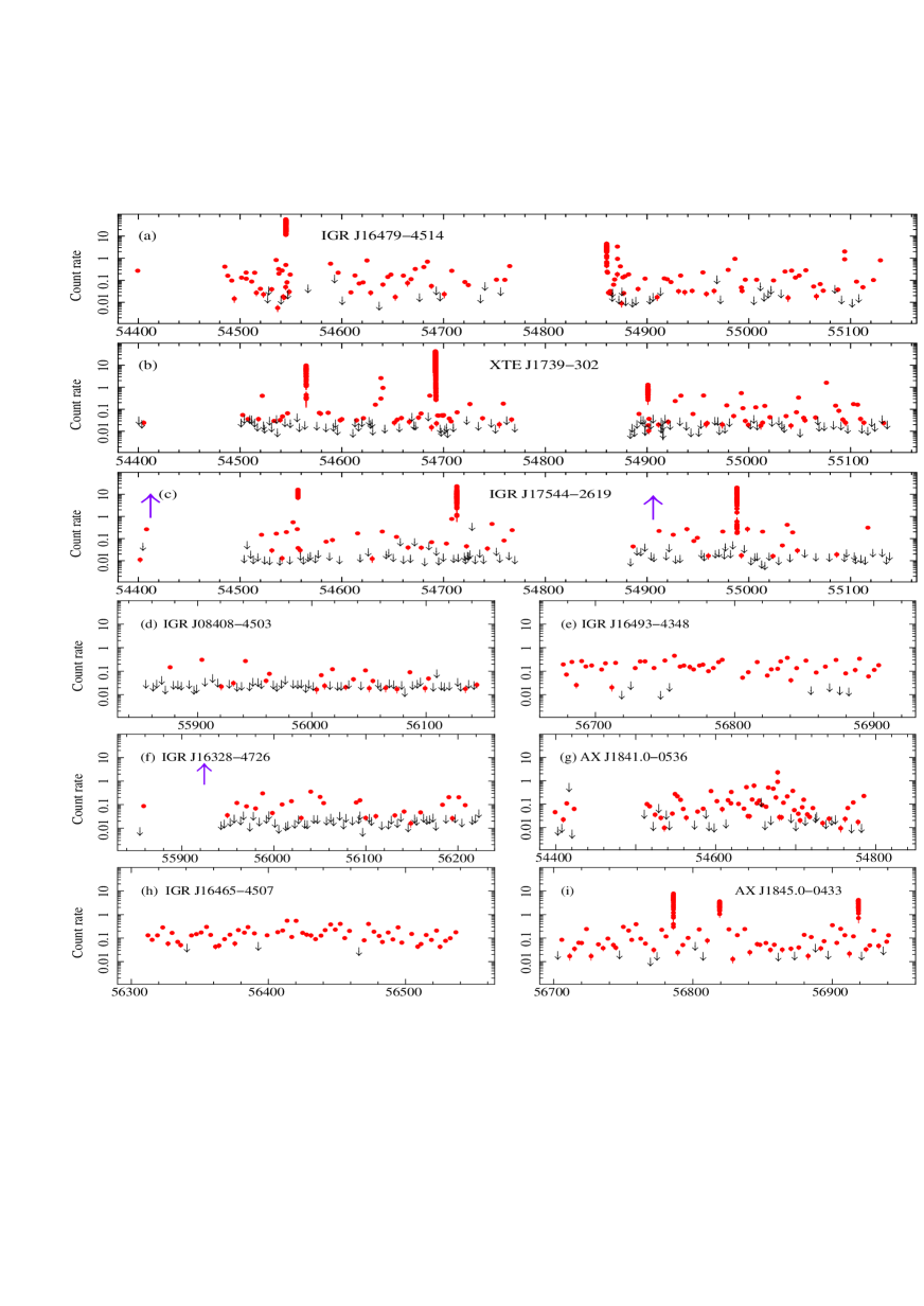
Figure 1: Swift/XRT (0.2–10 keV) long term light curves for the yearly monitoring sample. The x-axis is in MJD. The points refer to the average count rate measured for each observation except for outbursts, where the data were binned to include at least 20 counts bin^-1 (to best represent the dynamic range). Red points are detections, black downward-pointing arrows are 3-$\sigma$ upper limits. Violet upward-pointing arrows mark bright outbursts detected by BAT (and not simultaneously followed by XRT), or by MAXI (for AX J1841.0$-$0536). The data on IGR J16493$-$ 4348 (panel e) and AX J1845.0$-$0433 (panel i) are presented here for the first time. The remainder of the data are adapted from papers listed in Table 1 (Col. 17).

The first experiment within the Swift SFXT Project was performed in February 2007 (Romano et al. 2007) when we took advantage of the fact that at least one SFXT, IGR J11215$-$5952 (hereon J11215), showed outbursts with a periodicity of about 330 d (Sidoli et al. 2006) in the INTEGRAL data, and monitored one outburst with the Swift/X-ray Telescope (XRT, 0.2–10 keV, Burrows et al. 2005) from before onset, to the peak, and until it became undetectable with reasonable XRT exposures. The campaign lasted 23 d (total exposure of $\sim 73$ ks) and showed that, differently from previously thought based on lower-sensitivity instruments observing only the brightest hr-long flares (e.g. the hard X-ray monitor on board INTEGRAL), the soft X-ray emission, hence the accretion phase, lasted several days. Superimposed on the light curve, frequent flares are also observed, probably due to inhomogeneous accretion, i.e. clumps in the accreting wind. This phenomenology is consistent with a gradually increasing flux at the periastron passage in a wide eccentric orbit.

Swift also allowed the determination of the true orbital period $P_{\rm orb}\sim 164.6$ d (Sidoli et al. 2007; Romano et al. 2009c), a rare instance, as orbital periods are generally found from all-sky monitor data.

Furthermore, since the outbursts of this source are periodic and regularly spaced, and a non negligible eccentricity is required to account for the observed low quiescent luminosity, these data led Sidoli et al. (2007) to propose the existence of a second wind component from the supergiant companion in addition to its normal symmetric polar wind. This equatorially enhanced wind component is probably clumpy, denser and slower than the polar one, and inclined with respect to the orbital plane (to account for the narrowness of the outburst X-ray light curve).

2.2 Long term properties from monitoring campaigns

In the wake of the success of the J11215 campaign, during the Fall 2007 we selected 4 SFXTs from the 8 known at the time, IGR J16479$-$4514, XTE J1739–302, IGR J17544$-$2619, and AX J1841.0$-$0536 (hereon J16479, J1739, J17544, and J1841, respectively, the seed of our yearly sample, see Table 1), and set to perform a systematic study (Sidoli et al. 2008) with a year-long series of 1–2 ks pointed observations with XRT. At the time, the SFXT binary periods were largely unknown and believed to be in excess of 10 d (see the current status in Table 1, Col. 2), so the observations were scheduled 3–4 days apart. The initial goals were to i) seek for the signatures of equatorial winds, ii) catch outbursts to determine whether they showed any periodicities, iii) follow the sources during the whole outburst duration, and iv) monitor the quiescence.

For this project, the Swift/Burst Alert Telescope (BAT, 15–150 keV, Barthelmy et al. 2005) Team applied the “BAT special functions” to the sample of SFXTs and candidates (i.e., sources with similar X-ray flaring behaviour but with no firm measurement of the spectral type of the companion). This allowed Swift to react to an increase in flux from any SFXTs as if they were a GRB. In this way, whenever an SFXT triggers the BAT, simultaneous broad band data are collected that span $\sim 1600$–6000 Å through the UV/Optical Telescope (UVOT, Roming et al. 2005), and 0.2–150 keV through XRT and BAT combined.

Before we began our investigation, deep XMM–Newton exposures (González-Riestra et al. 2004) reporting fluxes between $\sim 10^{-13}$ and $10^{-10}$ erg s^-1 had described the characteristics of J17544 away from the bright outbursts, including a trend for harder spectra at higher fluxes, while a revealing Chandra observation (in’t Zand 2005) had caught the first detection of a fast X-ray transient in quiescence, a state characterized by a very soft (photon index $\Gamma=5.0\pm 1.2$) spectrum. On the other hand, the long-term behaviour of SFXTs, not unlike any other hard X-ray transient, had been traditionally investigated only with coded-mask large field-of-view instruments, such as INTEGRAL/IBIS (Ubertini et al. 2003) or Swift/BAT which, because of their sensitivity limits, mostly catch only the brightest portion of any transient event (see Romano et al. 2014c, for a catalogue of more than a thousand Swift/BAT bright SFXT flares described in Sect. 2.5). Therefore, our strategy, by combining sensitive soft X-ray monitoring with outburst follow-ups, has allowed us through the years for the first time, to systematically assess the soft X-ray long term properties of a conspicuous fraction of the SFXT sample when away from the prominent bright outbursts, in particular, the states leading down to quiescence.

The detailed results on the first campaigns can be found in Sidoli et al. (2008) and Romano et al. (2009b, 2011a), those on 3 more sources, IGR J08408$-$4503, IGR J16328 $-$4726, and IGR J16465$-$4507 (hereon J08408, J16328, and J16465) in Romano et al. (2014a). Table 1 reports the characteristics of the sources in our SFXT sample (binary period and distance, Cols. 2 and 3) and the campaign dates (Cols. 4 and 5). In the following, we summarize the results for these sources and introduce the new ones for J16493 and J1845, that were observed in 2014.

Fig. 1 shows the XRT light curves of the yearly sample at a daily resolution. The following can be observed:

1. The most striking features are, of course, the bright outbursts, which will be described in detail in Sect. 2.4. These outbursts, surprisingly, are however merely the tip of the iceberg in the SFXT activity (only a few percent of the total time).

2. All sources display a dynamic range (DR) of $\sim 3$–4 orders of magnitude.

3. The exceptions to the previous points are J16465 and the newly observed J16493, the latter showing a DR$\sim 48$. These two sources (Fig. 1h and 1e, respectively), based on their small DR, are therefore found to be not SFXTs, but classical systems.

4. For SFXTs, most of the emission is found outside the bright outbursts, so that the long-term behaviour of SFXTs is not quiescence but an intermediate state with an average X-ray luminosity of $10^{33}$–$10^{34}$ erg s^-1 (and, as reported below, a spectrum that can be fit with a power law with photon index $\Gamma=1$–2).

5. Variability is observed at all timescales we can probe. Superimposed on the day-to-day variability, we measure intra-day flaring that involves flux variations up to one order of magnitude; we identify flares down to a count rate in the order of 0.1 counts s^-1 ($L\sim 2$–$6\times 10^{34}$ erg s^-1) within a snapshot of about 1 ks.

As shown by Walter & Zurita Heras (2007) the short time scale variability cannot be accounted for by accretion from a homogeneous wind, but it can naturally be explained by the accretion of single clumps in the donor wind. We calculated that the average clump mass is $M_{\rm cl}\sim 0.3$–$2\times 10^{19}$ g (Romano et al. 2011a), about those expected (Walter & Zurita Heras 2007) to be responsible for short flares, below the INTEGRAL detection threshold and which, if frequent enough, may significantly contribute to the mass-loss rate.

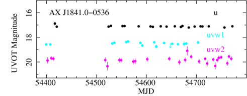
Figure 2: Swift/UVOT light curves of AX J1841.0$-$0536. Adapted from Romano et al. (2009b).

The data collected during these campaigns were used to perform soft X-ray intensity-selected spectroscopy. We find that the common out-of-outburst spectroscopic properties are a non-thermal emission (power law with $\Gamma=1$–2) combined with a soft excess becoming increasingly more dominant as the source flux state becomes lower, and a ubiquitous harder-when-brighter trend (Romano et al. 2009b, 2011a, 2014a). Therefore, the spectral modelling of out-of-outburst emission shows that accretion is occurring down to very low luminosities. This is clearly at odds with what is generally observed in the hard X-rays, due to the different instrumental sensitivities involved. Since a non-thermal spectrum plus a soft excess is common in classical systems, the spectroscopic properties are not an efficient method for discriminating SFXTs within the HMXB sample, differently from what happens for the dynamic range.

We note that when combining single 1–2 ks snapshots in which no detection was individually achieved, the XRT data can reach luminosities comparable to the quiescent one (Romano et al. 2009b). For instance, in the cases of J17544 and J1739 (Romano et al. 2011a) and J08408 (Romano et al. 2014a), luminosities of a few $10^{32}$ erg s^-1, have been reached, and the spectral properties observed in this very low state are consistent with those observed with deep XMM–Newton exposures (e.g. Bozzo et al. 2010).

UVOT observed simultaneously with the XRT during most of our monitoring with different combinations of optical and UV filters, depending on the magnitude of the companion stars (Romano et al. 2009b, 2011a). In J1739, only marginal variability was observed in the $u$ and $uvw1$ filters; the $uvw1$ light curve of J17544 and the $u$ and $uvw1$ light curves of J1841 were remarkably stable, consistently with the optical/UV emission being dominated by the constant contribution of the supergiant companions. Fig. 2 shows, as an example, the UVOT light curves of J1841.

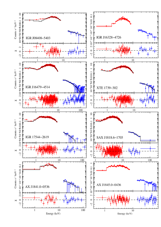
Figure 3: Swift/XRT and BAT simultaneous spectroscopy. Filled (red) circles and empty (blue) circles denote XRT and BAT data, respectively. The data are fit with an absorbed power law with a high energy cut-off model or absorbed power laws with high energy exponential cut-off model. Data references: IGR J08408$-$4503 (2008-07-05, Romano et al. 2009a); IGR J16328$-$4726 (2009-06-10, Romano et al. 2013); IGR J16479$-$4514 (2008-03-19, Romano et al. 2008); XTE J1739$-$302 (2008-08-13, Sidoli et al. 2009a); IGR J17544$-$2619 (2009-06-06, Romano et al. 2009b); SAX J1818.6$-$1703 (2009-05-06, Sidoli et al. 2009b); AX J1841.0$-$0536 (2010-06-05, Romano et al. 2011b); AX J1845.0$-$0433 (2012-05-05, Romano et al. 2013).

  

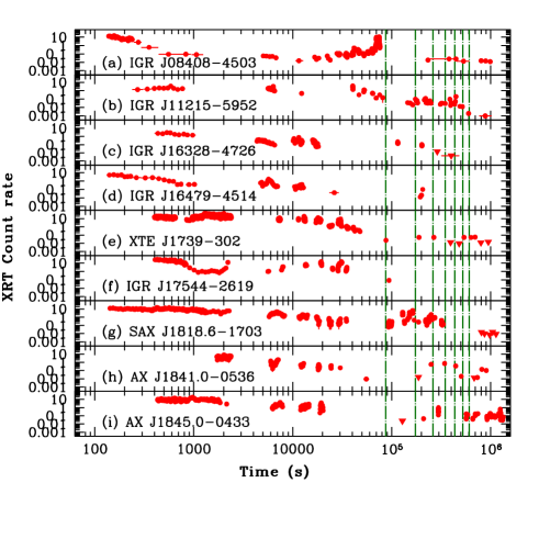
Figure 4: Swift/XRT light curves of the better followed-up outbursts of confirmed SFXTs, referred to their respective BAT triggers (except: IGR J11215$-$5952 is referred to MJD 54139.94). Points mark detections, triangles 3$\sigma$ upper limits, vertical dashed lines mark daily intervals, up to a week. Data references: IGR J08408$-$4503 (2008-07-05, Romano et al. 2009a); IGR J11215$-$5952 (2007-02-09, Romano et al. 2007); IGR J16328$-$4726 (2009-06-10, Romano et al. 2013); IGR J16479$-$4514 (2005-08-30, Sidoli et al. 2008); XTE J1739$-$302 (2008-08-13, Sidoli et al. 2009a); IGR J17544$-$2619 (2010-03-04, Romano et al. 2011b); SAX J1818.6$-$1703 (2009-05-06, Sidoli et al. 2009b); AX J1841.0$-$0536 (2010-06-05, Romano et al. 2011b); AX J1845.0$-$0433 (2012-05-05, Romano et al. 2013). Adapted from Romano et al. (2013).

2.3 Orbital monitoring campaigns

Further monitoring campaigns were also performed on three more sources with higher-cadence pointed observations (several XRT snapshots a day to provide intra-day sampling) for one or more orbital periods with the main goal of studying the effects of orbital parameters on the observed flare distributions. In 2009 we performed the very first complete monitoring of the soft X-ray activity along an entire orbital period ($P_{\rm orb}\sim 18.5$ d) of an SFXT, IGR J18483$-$0311 (J18483, Romano et al. 2010). Similarly, in 2011 we monitored the candidate SFXT IGR J16418$-$4532 (J16418, Romano et al. 2012) which has a much shorter orbital period, $P_{\rm orb}\sim 3.74$ d and, in 2012, the (then candidate) SFXT IGR J17354$-$3255 (J17354), with $P_{\rm orb}=8.4474$ d (Ducci et al. 2013b). These three sources compose our orbital monitoring sample.

These unique datasets allowed us to constrain in these objects the different mechanisms proposed to explain their nature. In particular, we applied the clumpy wind model for blue supergiants (Ducci et al. 2009) to the observed X-ray light curve. By assuming for J18483 an eccentricity of $e=0.4$ and for J16418 circular orbits, we could explain their X-ray emission in terms of the accretion from a spherically symmetric clumpy wind, composed of clumps with different masses, ranging from $10^{18}$ to $\times 10^{21}$ g for J18483, and from $\sim 5\times 10^{16}$ g to $10^{21}$ g for J16418. Since J18483 is an intermediate SFXT with a moderately high dynamic range in the X-ray luminosity, the estimated sizes and masses of the clumps in J18483 are somewhat larger that what would be expected according to the multidimensional simulations of massive stars winds (Dessart & Owocki 2002, 2003, 2005) but likely not unrealistic (see, e.g. Fürst et al. 2014). The addition of magnetic/centrifugal gates could lower the requirements on the clump sizes and masses, but such mechanisms cannot be readily applied to the case of J18483 as the magnetic field of the NS hosted in this source and its spin period are highly debated (e.g. Ducci et al. 2013a; Sguera et al. 2015). We found that J17354 is probably a wind-fed system and that the dip observed in its light curve cannot be explained with a luminosity modulation due to a highly eccentric orbit; on the contrary, it can be explained in terms of an eclipse or the onset of gated mechanisms.

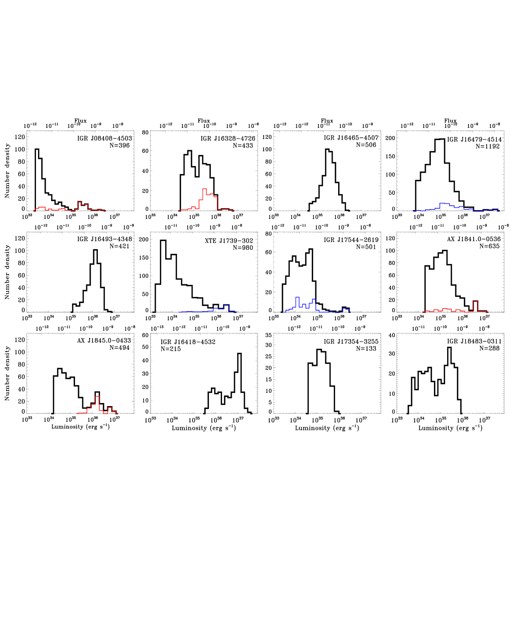
Figure 5: Differential distributions of the 2–10 keV luminosity (lower axis) and flux (unabsorbed, upper axis) drawn from the Swift/XRT light curves binned at 100 s. N is the sample size. The thick black lines represent the data collected during the monitoring campaigns (see Table 1, Col 4 and 5 for the campaign dates). The thin blue histograms show the part of the data collected as outburst observations during the campaign, thus including both the initial bright flare and the follow-up observations (see Sect. 3). The thin red histograms show outburst observations collected outside of the monitoring campaign (one outburst per source). The data on IGR J16493$-$4348 and AX J1845.0$-$0433 are presented here for the first time, the rest are adapted from Romano et al. (2014a).

2.4 SFXT broad-band properties and arcsecond localizations from outbursts and outburst follow-ups

Since Swift is a GRB-chasing mission, provided with fast automated slewing and panchromatic sensitivity, once SFXTs were included in the BAT special functions (see Sect. 2.2), SFXT outbursts started triggering the BAT and narrow field instrument (NFI) data (XRT and UVOT) started being collected within a few hundred seconds (down to about $\sim 100$ s) from the BAT trigger. The shape of the SFXT spectrum in outburst is a power law with an exponential cutoff at a few keV, therefore the large Swift energy range can both help constrain the hard-X spectral properties (to compare with popular accreting neutron star models) and measure the absorption.

These simultaneous XRT and BAT data allowed us to perform, for the first time, simultaneous broad band spectroscopy of an SFXT in outburst (J16479, Romano et al. 2008). At the time of writing, we have collected a total of 51 bright flares (55 triggers, of which 4 double) that triggered the BAT, more than half of which followed-up with the NFI, thanks to the BAT special functions, so that we have been able to observe in this fashion most of the SFXT sample, as shown in Fig. 3. We found out that for all sources a good fit could indeed be obtained with a power-law with an exponential cutoff. This, in turn implies, based on the cutoff energy, a magnetic field consistent with a few $10^{12}$ G, typical of accreting NSs in HMXBs.

The availability of such data also motivated the development of a physical model, compmag in XSPEC (Farinelli et al. 2012a), which includes thermal and bulk Comptonization for cylindrical accretion onto a magnetized neutron star. A full description of the algorithm (see Farinelli et al. 2012a) is beyond the scope of this paper but the model has been successfully applied to the SFXT class prototypes J17391 and J17544 (Farinelli et al. 2012b), and to J18483 (Ducci et al. 2013a).

An important benefit of NFI observations is Swift’s ability to provide arcsecond localization for several SFXTs and candidates whose coordinates were only known to the arcminute level, or to improve on previously known coordinates (e.g. Kennea et al. 2005; Grupe et al. 2009). This greatly helps in associating with optical counterparts.

Our observing strategy also includes XRT follow-ups for days (generally up to a week) after the outburst via ToO observations, well after it had become undetectable with monitoring instruments with lower sensitivity. Fig. 4 shows the best examples of outburst light curves as observed by XRT, and exemplifies the common X-ray characteristics of this class:

• extended soft X-ray activity around an outburst lasting up several days (see the vertical lines in Fig. 4);

• a multiple-peaked structure;

• a DR (only including bright outbursts) up to $\sim 3$ orders of magnitude.

2.5 The 100-month SFXT BAT catalogue and the number of SFXTs in the Galaxy

Since BAT observes an average of 88% of the sky daily, it is ideally suited to detect flaring hard X-ray astrophysical sources, SFXTs in particular. We have thus produced the 100-month Swift Catalogue of SFXTs (Romano et al. 2014c) which collects over a thousand BAT flares from 11 SFXTs, and reaches down to 15–150 keV fluxes of about $6\times 10^{-10}$ erg cm^-2 s^-1 (daily timescale) and about $1.5\times 10^{-9}$ erg cm^-2 s^-1 (Swift orbital timescale). We found that these hard X-ray flares typically last at least a few hundred seconds, reach above 100 mCrab (15–50 keV), and last much less than a day. Their clustering in the binary orbital phase-space, however, demonstrates that these short flares are part of much longer outbursts, lasting up to a few days, as previously observed during our outburst follow-ups (Sect. 2.4). This large dataset can therefore probe the high and intermediate emission states in SFXTs, and help infer the properties of these binaries; it can also be used to estimate the number of flares per year each source is likely to produce as a function of the detection threshold and limiting flux in future missions. Finally, the catalogue has recently been exploited by Ducci et al. (2014) to estimate the expected number of SFXTs in the Milky Way, $N\approx 37{+53\atop-22}$. This shows that SFXTs constitute a large portion of X-ray binaries with supergiant companions in the Galaxy.

3 Differential luminosity distributions

An often understated property of the monitoring data is that the yearly campaigns are statistically representative of the long-term soft X-ray properties of SFXTs that the deep exposures from pointed telescopes can only rarely and non-uniformly sample. Our observations are also independent, since each observation is not triggered by the preceding ones (we consider the outburst followups as a separate set of data when in need of a statistical set). Our monitoring pace thus provides a casual sampling of the soft X-ray light curve at a resolution of $\sim 3$–4 d over a baseline of one or two years, therefore it offers both coverage of a large number of binary orbital cycles (ranging from $\sim 15$ cycles for J17391 to $\sim 220$ for J164794) and a good sampling of the orbital phase (see fig. 6 of Romano et al. 2014a).

Based on these premises, we can effectively calculate the percentage of time each source spent in different flux states, among which we distinguish:

1. the flares that trigger the BAT (see Sect. 2.4) accounting for 3–5 % of the exposure time;

2. the intermediate states (all observations yielding a firm detection excluding outbursts);

3. non detections (significance below 3$\sigma$; see Sect. 4). Only observations with an exposure in excess of 900 s were considered to account for non detections obtained during very short exposures (due to our observations being interrupted by a higher figure-of-merit GRB). These correspond to flux limits $F_{\rm 2-10\,keV}^{\rm lim}\sim(1$–$3)\times 10^{-12}$ erg cm^-2 s^-1 (see Col. 9 of Table 1, and also the corresponding limits in count rates, Col. 8, and luminosity, Col. 10).

From the XRT light curves binned at 100 s, of both the yearly and the orbital monitoring samples, and after removing the observations where a detection was not achieved (thus selecting only the intermediate states), we construct the 2–10 keV differential luminosity distributions (DLD), shown in Fig. 5 (solid black lines). For all sources we adopted a single conversion factor between count rates, fluxes and luminosities, that were derived from the ‘medium’ spectrum for J16465, J16479, J16493, J1739, J17544, J1841, J1845, and J18483, the ‘low’ spectrum for J08408 and J16328, the first observation for J16418, and the average spectrum for the weak source J17354 (Romano et al. 2010, 2011a, 2012; Ducci et al. 2013b; Romano et al. 2014a). Because the uncertainty in this conversion is dominated by those on the distance (Table 1, Col. 3), the top x-axis of Fig. 5 also reports the flux scale in the same energy band. We note that the DLDs drawn from the orbital monitoring sample need to be taken with caution, as they follow an entirely different observing strategy. These observations were in fact collected with intensive campaigns during one or a few orbital periods, as opposed to the few points per each period typical of the yearly campaign data, so short timescale variability may play an important role.

Fig. 5 distinguishes (as a thin blue line) the data that were taken during an outburst that occurred during the observing campaign (two for J16479, and three for J1739 and J17544), and those (thin red line) of outbursts that were observed outside of the campaigns (we considered one for each of J08408, J16328, J1840, and J1845).

The DLD of the SFXT prototypes, J1739 and J17544, as well as J16479 and J08408 show two distinct populations of flares. The first one is due to the outburst emission (peaking/reaching a few $10^{-9}$ erg cm^-2 s^-1), the second is due to the out-of-outburst emission, characterized by emission spanning up to 4 orders of magnitude in DR (at 100 s binning). This also applies to the newly observed J18450, which also shares a DR of at least 3 orders of magnitude at a temporal resolution of 100 s. We cannot exclude that particular distributions of the clump and wind parameters may produce a double-peaked DLD (Romano et al. 2014a), but this behaviour is more easily explained in terms of different accretion regimes as predicted by the magnetic/centrifugal gating model or the quasi-spherical settling accretion model (Grebenev & Sunyaev 2007; Bozzo et al. 2008; Shakura et al. 2012, 2013).

The classical systems (J16465 and the newly observed J16493), on the contrary, only show one peak in their DCD, which is significantly brighter than those of of SFXTs. This confirms the findings of Lutovinov et al. (2013) that SFXTs show a median luminosity beneath the one of normal wind-fed HMXBs; the flaring observed in SFXTs can therefore be explained if some mechanism, such as magnetic arrest, can inhibit accretion. DCDs, therefore, can be used effectively to discriminate between the most extreme SFXTs, the intermediate systems, and classical systems.

While the outbursts account for 3 and 5 % of the exposure time, the most probable flux level at which a random observation will find these sources, when detected, can be retrieved from the peak of the DLD, and this is of course a powerful tool to plan further observing campaigns, as is the distribution of detections along the orbital phase (see fig. 6 of Romano et al. 2014a). In particular, in Fig. 6 we show the case of J17544 which flares tend to cluster around periastron more than in other SFXTs.

Figure 6: Distribution of the XRT detections (count rates) of IGR J17544$-$2619 (0.2–10 keV) folded at the orbital period, based on the most recent outburst ephemeris for this source ($P=4.92693\pm 0.00036$ d, periastron at MJD $53732.65\pm 0.23$; Smith 2014).

4 Inactivity duty cycles

The duty cycle of astrophysical sources is usually defined as the fraction of time the sources are active, and it is used to both characterize their emission properties and and to plan further observing campaigns to study them. SFXTs, however, show a very large dynamical range, with activity observed by the XRT spanning several orders of magnitude in flux. It is more interesting, therefore, to define a measurement of inactivity as opposed of one of activity.

From the non detections, we define the inactivity duty cycle (Romano et al. 2009b) as the time each source spends undetected down to a flux limit of 1–3$\times 10^{-12}$ erg cm^-2 s^-1,

$${\rm IDC}=\Delta T_{\Sigma}/[\Delta T_{\rm tot}\,(1-P_{\rm short})]\,,$$ (1)

where $\Delta T_{\Sigma}$ is the sum of the exposures (each longer than 900 s) accumulated in all observations where only a 3$\sigma$ upper limit was achieved (Table 1, Col. 11), $\Delta T_{\rm tot}$ is the total exposure accumulated (Table 1, Col. 7), and $P_{\rm short}$ is the fraction of time lost to short observations (exposure $<900$ s, Table 1, Col. 12). The cumulative count rate for each object is also reported Table 1 (Col. 14).

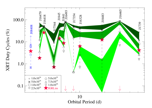
Figure 7: The XRT duty cycle (2–10 keV) as a function of orbital period and for a range of 2–10 keV luminosities (see legend, in units of erg s^-1) in black. Only points above 0.1 % are shown. Since the period of J08408 is currently unknown (see Table 1 Col. 2 for the values adopted for the rest of the sample), we arbitrarily place it at an orbital period of about two days and mark it in blue. The shaded areas mark the loci of the XRT duty cycle defined by contiguous luminosities. The red filled stars represent the XRT duty cycle at the INTEGRAL sensitivity for each object (the downward-pointing arrows are consistent with 0). The data on IGR J16493$-$4348 and AX J1845.0$-$0433 are presented here for the first time, the rest are adapted from Romano et al. (2014a).

The need to provide uncertainties on IDCs by avoiding the standard approach of deriving them from extensive and time-consuming Monte Carlo bootstrap simulations has lead us to propose an application of Bayesian techniques, instead (Romano et al. 2014b). We exploited the fact that SFXTs are, when considering duty cycles, two-state sources, since they can only be found in either of two possible, mutually exclusive states, inactive (off) or flaring (on). Or, in this case, above or below a given flux threshold. We derived the theoretical expectation value for the duty cycle and its error as based on a finite set of independent observational data points following a Bayesian approach (Romano et al. 2014b). The IDCs and their uncertainties thus calculated are reported in Table 1, Col. 13.

We note that IDCs can be quite small for classical systems, which are to all extents and purposes persistent sources, and because they are on average more luminous. Once again, IDCs can help discriminate between SFXTs, intermediate and classical systems.

5 Discussion: the seventh year crisis

In the following, we discuss the “seventh year crisis”, the challenges that the recent observations (those collected by Swift, in primis) are making to the prevailing models attempting to explain the SFXT behaviour.

Duty Cycles and orbital geometry. If the properties of the binary geometry and inhomogeneities of the stellar wind from the primary were the leading causes of the observed X-ray variability in SFXTs, as initially proposed in clumpy wind models (e.g. in’t Zand 2005; Negueruela et al. 2008; Walter & Zurita Heras 2007), generally larger IDCs would be expected for longer orbital periods. Naturally, the definition of duty cycle is strongly dependent on the luminosity assumed as lower limit for the calculation. Therefore, we exploited the high sensitivity afforded by the XRT observations and defined an XRT luminosity-based duty cycle (XRTDC) as the percentage of time the source spends above a given luminosity. We considered several (2–10 keV) luminosities in the range $L_{\rm 2-10\,keV}=10^{34}$–$10^{36}$ erg s^-1 and included the particular value of the luminosity corresponding to the INTEGRAL sensitivity for each object.

Figure 7 shows the XRTDC as a function of the orbital period with red stars marking the value at the INTEGRAL sensitivity. No clear correlation is found between the orbital periods and any of the duty cycles. This implies that wide orbits are not characterized by low duty cycles, as the clumpy wind models would predict. An intrinsic mechanism instead seems to be more likely responsible for the observed variability in SFXTs, i.e., either the wind properties or the compact object properties. However, it is hard to justify the radically different wind properties in SFXTs from those in classical systems with the same companion spectral type. Therefore, in light of this lack of correlation with the orbital period and our finding distinct flare populations (see Sect. 3), it seems more plausible that accretion-inhibition mechanisms or a quasi-spherical settling accretion regime may be in action, instead.

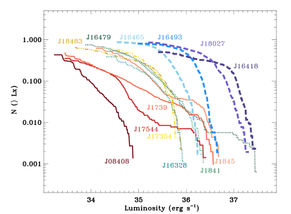
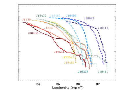
Figure 8: Cumulative luminosity distributions of the 2–10 keV luminosity drawn from the Swift/XRT light curves binned at 100 s. The classical SGXB IGR 18027$-$2016 is marked with a thick dashed line. Newly classified classical systems IGR J16465$-$4507, IGR J16418$-$4532, and IGR J16493$-$4348 are also marked with thick dashed lines. The intermediate SFXTs IGR J18483$-$0311 and IGR J17354$-$3255 are shown as dot-dashed lines. IGR J16328$-$4726, IGR J16479$-$4514, and AX J1841.0$-$0536 are shown as dotted lines, while the most extreme SFXTs (IGR J08408$-$4503, XTE J1739$-$302, IGR J17544$-$2619, and AX J1845.0$-$0433) are marked with solid lines. The data on IGR J16493$-$4348 and AX J1845.0$-$0433 are presented here for the first time, the rest are adapted from Bozzo et al. (2015). Left: Only XRT data collected during the monitoring campaigns of all sources are used. Right: Same as for the left, but in this case we also considered one outburst for the sources IGR J08408$-$4503, IGR J16328$-$4726, AX J1841.0$-$0536, and AX J1845.0$-$0433 recorded by the XRT outside the corresponding monitoring campaigns.

Cumulative luminosity distributions. In Sect. 3 and 4 we have shown that DLDs and IDCs can be used effectively to discriminate SFXTs from classical systems, since the former are characterized by lower average luminosities. Another way to examine this property is to use the cumulative luminosity distributions (CLD) for our sample as calculated from the long term monitoring data (Sect. 3). In Bozzo et al. (2015) the CLDs of the SFXT sample, as well as that of the classical SGXB IGR J18027 $-$2016 (J18027), are reported in the soft X-rays. Previous work constructed CLDs based on the RXTE Galactic bulge scan programme data (Smith et al. 2012) and INTEGRAL long-term monitoring (Paizis & Sidoli 2014). In Fig. 8, in which we also added the newly observed J16493 and J1845, the CLDs are normalized to the total exposure for each source, so that the source duty cycle corresponds to the highest value on the y-axis. We can see that classical systems are characterized by CLDs with a single knee at $\sim 10^{36}$–$10^{37}$ erg s^-1. On the contrary, SFXTs are systematically sub-luminous, with their CLDs shifted at 100–100 times lower luminosities.

As shown in Fig. 8, the classical SgXRB J18027 (thick dashed line) is characterized by a single knee at $\sim 10^{36}$ erg s^-1. The CLDs of J16465, J16418, and J16493 (thick dashed lines) closely resemble that of classical systems, with a position of the knee that can be accounted for once the relative distances and dependence of the flux from the orbital periods are considered. As done in Bozzo et al. (2015) for the former two, we here reclassify the newly observed SFXT candidate J16493 as a classical system. The intermediate SFXTs J18483 and J17354 (dot-dashed lines) have CLDs similar to those of classical systems, but shifted at ten times lower luminosities. The CLDs of J16328, J16479, and J1841.0 (dotted lines), are characterized by even lower luminosities (one can note the similarity of the orbital periods of J16479 and J16418, and that of J16328 to Vela X-1). The profiles show more complexity, as more knees are appearing, reflecting different peaks in the DLDs, that is, different population of flares. Finally, the most extreme SFXTs, J08408, J1739, J17544, and the newly observed J1845.0 (solid lines) show very complex profiles.

Considering that both differential/cumulative distributions and inactivity duty cycles show that SFXTs are underluminous when compared to HMXBs, and that single knee profiles in CLDs can be understood in terms of wind accretion from an inhomogeneous medium (see, e.g. Fürst et al. 2010), we can interpret the differences observed between classical systems and SFXTs as due to accretion from a structured wind in the former sources and to the presence of magnetic/centrifugal gates or a quasi-spherical settling accretion regime in the latter.

The king, the power and the ring. Ruler of a small kingdom, the SFXT prototype J17544 has been a stimulus, a catalyst, and a continuous challenge in the process of understanding SFXTs as a class since it was discovered by INTEGRAL over ten years ago (Sunyaev et al. 2003). The optical counterpart in this binary (orbital period $P_{\rm orb}=4.926\pm 0.001$ d, Clark et al. 2009) is quite an ordinary O9Ib star with a mass of 25–28 $M_{\odot}$ (Pellizza et al. 2006) and located at a distance of 3.6 kpc (Rahoui et al. 2008). The large luminosity swings observed on timescales as short as hours were alternatively explained by mechanisms that regulate or inhibit accretion (Stella et al. 1986; Grebenev & Sunyaev 2007, propeller effect; Bozzo et al. 2008, magnetic gating). In particular, Bozzo et al. (2008) explained them in terms of transitions across the magnetic and/or centrifugal barriers. In this scenario, the large dynamic range of SFXTs (about five decades) is achieved with a small variation of the mass loss rate (e.g. a factor of $\sim$5 in fig. 3a of Bozzo et al. 2008) by assuming a spin period $P_{\rm spin}$ in excess of $\sim 1000$ s and a magnetar-like field ($B\geq 10^{14}$ G). A recent NuSTAR observation (Bhalerao et al. 2015), however, has revealed a cyclotron line at 17 keV, yielding the first measurement of the magnetic field in a SFXT, at $\sim 1.5\times 10^{12}$ G, typical of accreting NSs in HMXBs. This set of observations therefore rule out the magnetar nature for the SFXT prototype.

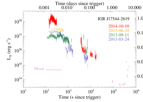
Figure 9: Bolometric X-ray luminosity light curves of the brightest outbursts recorded by Swift for IGR J17544$-$2619. The giant burst of 2014 October 10 is shown in red, and compared with previous bright outbursts from this source. The horizontal (pink) line marks the average level for this source, obtained from the two year monitoring campaign (Romano et al. 2011a, see Sect. 2.2), while the right-hand y-axis is the standard Eddington luminosity for spherical accretion of fully ionized hydrogen for a 1.4 M_⊙ NS. Adapted from Romano et al. (2015).

On the other hand, the propeller and gating models are still applicable to fast rotators ($P_{\rm spin}<10^{3}$ s) even with non-magnetar magnetic fields like those observed in classical systems. Grebenev (2010) provided a simple equation to estimate the neutron star spin period at which the magnetic inhibition regime takes place,

$$P_{\rm spin}\approx 4.5B_{12}^{6/7}\dot{M}_{-5}^{-3/7}v_{3}^{12/7}P_{10}^{4/7}~{}{\rm s},$$

where $B_{12}=B/10^{12}$ G is the magnetic field of the neutron star, $\dot{M}_{-5}=\dot{M}_{\rm w}/10^{-5}$ M_⊙ yr^-1 and $v_{3}=v_{\rm w}/10^{3}$ km s^-1 are the mass loss rate and the wind velocity of the donor star, and $P_{10}=P_{\rm orb}/10$ d is the orbital period (see also fig. 4 of Grebenev 2010). Bozzo et al. (2008) showed that for sub-magnetar fields and $\lesssim 100$ s spinning neutron stars, a $10^{5}$ luminosity swing would require a much higher increase in the mass loss rate with respect to the magnetar case (a factor of $\sim 100$ in fig. 4 of Bozzo et al. 2008). Such increase would imply that, either the mass loss rate from the supergiant stars in SFXTs changes abruptly on short time scales, or the local fluctuations in velocity and density of their winds are substantially larger than that of classical systems. In both cases, this would imply a fine tuning for the properties of the supergiant star winds in SFXTs compared to other SGXBs. At present, there is no observational evidence that this should be the case, as discussed in Bozzo et al. (2015).

While current investigations concentrate on finding possible mechanisms to inhibit accretion in SFXTs and to explain their unusually low average X-ray luminosity, J17544 seems to be testing our modelling further. An exceptionally bright outburst was observed by Swift on 2014 October 10 (Romano et al. 2015), during which the source reached a peak luminosity of $3\times 10^{38}$ erg s^-1 (or a 0.3–10 keV unabsorbed flux of $1.0\times 10^{-7}$ erg cm^-2 s^-1, corresponding to 2.1 Crab). Tentative evidence for pulsations at a period of $11.6$ s, and an expanding X-ray halo, or ring, around the source were also found in the XRT data. Such a high luminosity (see Fig. 9) not only extends the dynamic range of this source to DR$\sim 10^{6}$, a uniquely high value (by a factor of 10), but also reaches the standard Eddington limit expected for a NS of 1.4 $M_{\odot}$, thus challenging, for the first time, the maximum (rather than the minimum) theoretical luminosity expected for an SFXT. In Romano et al. (2015) we propose that this giant outburst could be caused by the formation of a transient accretion disc around the compact object.

Conclusions

In the last seven years, Swift  has contributed many “firsts” in the SFXT field, that I have summarized in this Paper; most importantly, it has performed the first systematic investigation of the soft X-ray long term properties of SFXTs with a vey sensitive instrument. This has provided us with many clues to help us understand SFXT outburst physics; it has revised or revolutionized incomplete or over-inferred properties derived from lower-sensitivity monitorings; it has motivated the creation of new models (both geometrical and physical) and helped test their applicability.

Swift has consistently surprised us with the unexpected. And yet, we are still missing some key ingredients to understand SFXT variability, especially when compared with classical systems. The current crisis is an excellent motivation to look “deeper and longer” and, in this framework, Swift  monitoring programs on SFXTs and classical HMXBs will be crucial.

References

- Barthelmy et al. (2005) Barthelmy, S. D., et al., 2005. SSRv 120, 143.
- Bhalerao et al. (2015) Bhalerao, V., et al., 2015. MNRAS 447, 2274.
- Bozzo et al. (2008) Bozzo, E., Falanga, M., Stella, L., 2008. ApJ 683, 1031.
- Bozzo et al. (2015) Bozzo, E., Romano, P., Ducci, L., Bernardini, F., Falanga, M., 2015. AdSpR 55, 1255.
- Bozzo et al. (2013) Bozzo, E., Romano, P., Ferrigno, C., Esposito, P., Mangano, V., 2013. AdSpR 51, 1593.
- Bozzo et al. (2010) Bozzo, E., Stella, L., Ferrigno, C., Giunta, A., Falanga, M., Campana, S., Israel, G., Leyder, J. C., 2010. A&A 519, A6.
- Burrows et al. (2005) Burrows, D. N., et al., 2005. SSRv 120, 165.
- Clark et al. (2009) Clark, D. J., Hill, A. B., Bird, A. J., McBride, V. A., Scaringi, S., Dean, A. J., 2009. MNRAS 399, L113.
- Coleiro & Chaty (2013) Coleiro, A., Chaty, S., 2013. ApJ 764, 185.
- Corbet et al. (2010) Corbet, R. H. D., Barthelmy, S. D., Baumgartner, W. H., Krimm, H. A., Markwardt, C. B., Skinner, G. K., Tueller, J., 2010. ATel 2588.
- Cusumano et al. (2010) Cusumano, G., La Parola, V., Romano, P., Segreto, A., Vercellone, S., Chincarini, G., 2010. MNRAS 406, L16.
- D’Aì et al. (2011) D’Aì, A., La Parola, V., Cusumano, G., Segreto, A., Romano, P., Vercellone, S., Robba, N. R., 2011. A&A 529, A30.
- Dessart & Owocki (2002) Dessart, L., Owocki, S. P., 2002. A&A 383, 1113.
- Dessart & Owocki (2003) Dessart, L., Owocki, S. P., 2003. A&A 406, L1.
- Dessart & Owocki (2005) Dessart, L., Owocki, S. P., 2005. A&A 437, 657.
- Drave et al. (2010) Drave, S. P., Clark, D. J., Bird, A. J., McBride, V. A., Hill, A. B., Sguera, V., Scaringi, S., Bazzano, A., 2010. MNRAS 409, 1220.
- Ducci et al. (2014) Ducci, L., Doroshenko, V., Romano, P., Santangelo, A., Sasaki, M., 2014. A&A 568, A76.
- Ducci et al. (2013a) Ducci, L., Doroshenko, V., Sasaki, M., Santangelo, A., Esposito, P., Romano, P., Vercellone, S., 2013a. A&A 559, A135.
- Ducci et al. (2013b) Ducci, L., Romano, P., Esposito, P., Bozzo, E., Krimm, H. A., Vercellone, S., Mangano, V., Kennea, J. A., 2013b. A&A, 556, A72.
- Ducci et al. (2009) Ducci, L., Sidoli, L., Mereghetti, S., Paizis, A., Romano, P., 2009. MNRAS 398, 2152.
- Farinelli et al. (2012a) Farinelli, R., Ceccobello, C., Romano, P., Titarchuk, L., 2012a. A&A 538, A67.
- Farinelli et al. (2012b) Farinelli, R., et al., 2012b. MNRAS 424, 2854.
- Fiocchi et al. (2013) Fiocchi, M., Bazzano, A., Bird, A. J., Drave, S. P., Natalucci, L., Persi, P., Piro, L., Ubertini, P., 2013. ApJ 762, 19.
- Fürst et al. (2010) Fürst, F., et al., 2010. A&A 519, A37.
- Fürst et al. (2014) Fürst, F., et al., 2014. ApJ 780, 133.
- Gehrels et al. (2004) Gehrels, N., et al., 2004. ApJ 611, 1005.
- González-Galán (2015) González-Galán, A., 2015. Fundamental properties of High-Mass X-ray Binaries, PhD Th., arXiv:1503.01087.
- González-Riestra et al. (2004) González-Riestra, R., Oosterbroek, T., Kuulkers, E., Orr, A., Parmar, A. N., 2004. A&A 420, 589.
- Goossens et al. (2013) Goossens, M. E., Bird, A. J., Drave, S. P., Bazzano, A., Hill, A. B., McBride, V. A., Sguera, V., Sidoli, L., 2013. MNRAS 434, 2182.
- Grebenev (2010) Grebenev, S. A., 2010. Supergiant Fast X-ray Transients observed by INTEGRAL, in The Extreme sky: Sampling the Universe above 10 keV, PoS, 96, 60, arXiv:1004.0293.
- Grebenev & Sunyaev (2007) Grebenev, S. A., Sunyaev, R. A., 2007. Astronomy Letters, 33, 149.
- Grupe et al. (2009) Grupe, D., Kennea, J., Evans, P., Romano, P., Markwardt, C., Chester, M., 2009. ATel 2075.
- in’t Zand (2005) in’t Zand, J. J. M., 2005. A&A 441, L1.
- Kennea et al. (2005) Kennea, J. A., Pagani, C., Markwardt, C., Blustin, A., Cummings, J., Nousek, J., Gehrels, N., 2005. ATel 599.
- La Parola et al. (2010) La Parola, V., Cusumano, G., Romano, P., Segreto, A., Vercellone, S., Chincarini, G., 2010. MNRAS 405, L66.
- Levine et al. (2011) Levine, A. M., Bradt, H. V., Chakrabarty, D., Corbet, R. H. D., Harris, R. J., 2011. ApJS 196, 6.
- Levine & Corbet (2006) Levine, A. M., Corbet, R., 2006, ATel 940.
- Lutovinov et al. (2013) Lutovinov, A. A., Revnivtsev, M. G., Tsygankov, S. S., Krivonos, R. A., 2013. MNRAS 431, 327.
- Negueruela et al. (2006) Negueruela, I., Smith, D. M., Reig, P., Chaty, S., Torrejón, J. M., 2006. 604, 165.
- Negueruela et al. (2008) Negueruela, I., Torrejón, J. M., Reig, P., Ribó, M., Smith, D. M., 2008. in AIP Conf. Ser., Vol. 1010, A Population Explosion: The Nature & Evolution of X-ray Binaries in Diverse Environments, ed. R. M. Bandyopadhyay, S. Wachter, D. Gelino, C. R. Gelino, 252–256.
- Nespoli et al. (2010) Nespoli, E., Fabregat, J., Mennickent, R. E., 2010. A&A 516, A106.
- Paizis & Sidoli (2014) Paizis, A., Sidoli, L., 2014. MNRAS 439, 3439.
- Pellizza et al. (2006) Pellizza, L. J., Chaty, S., Negueruela, I., 2006. A&A 455, 653.
- Rahoui et al. (2008) Rahoui, F., Chaty, S., Lagage, P.-O., Pantin, E., 2008. A&A 484, 801.
- Romano et al. (2015) Romano, P., et al., 2015. A&A 576, L4.
- Romano et al. (2014a) Romano, P., Ducci, L., Mangano, V., Esposito, P., Bozzo, E., Vercellone, S., 2014a. A&A 568, A55.
- Romano et al. (2014b) Romano, P., Guidorzi, C., Segreto, A., Ducci, L., Vercellone, S. 2014b. A&A 572, A97.
- Romano et al. (2014c) Romano, P., et al., 2014c. A&A 562, A2.
- Romano et al. (2011a) Romano, P., et al., 2011a. MNRAS 410, 1825.
- Romano et al. (2011b) Romano, P., et al., 2011b. MNRAS 412, L30.
- Romano et al. (2012) Romano, P., et al., 2012. MNRAS 419, 2695.
- Romano et al. (2013) Romano, P., et al., 2013. AdSpR 52, 1593.
- Romano et al. (2009a) Romano, P., et al., 2009a. MNRAS 392, 45.
- Romano et al. (2009b) Romano, P., et al., 2009b. MNRAS 399, 2021.
- Romano et al. (2009c) Romano, P., Sidoli, L., Cusumano, G., Vercellone, S., Mangano, V., Krimm, H. A., 2009c. ApJ 696, 2068.
- Romano et al. (2010) Romano, P., et al., 2010, MNRAS 401, 1564.
- Romano et al. (2007) Romano, P., Sidoli, L., Mangano, V., Mereghetti, S., Cusumano, G., 2007. A&A 469, L5.
- Romano et al. (2008) Romano, P., et al., 2008. ApJL, 680, L137.
- Roming et al. (2005) Roming, P. W. A., et al., 2005. SSRv 120, 95.
- Sguera et al. (2005) Sguera, V., et al., 2005. A&A 444, 221.
- Sguera et al. (2015) Sguera, V., Sidoli, L., Bird, A. J., Bazzano, A., 2015. MNRAS 449, 1228.
- Shakura et al. (2013) Shakura, N., Postnov, K., Hjalmarsdotter, L., 2013. MNRAS 428, 670.
- Shakura et al. (2012) Shakura, N., Postnov, K., Kochetkova, A., Hjalmarsdotter, L., 2012. MNRAS 420, 216.
- Shakura et al. (2014) Shakura, N., Postnov, K., Sidoli, L., Paizis, A., 2014. MNRAS 442, 2325.
- Sidoli et al. (2006) Sidoli, L., Paizis, A., Mereghetti, S., 2006. A&A 450, L9.
- Sidoli et al. (2009a) Sidoli, L., et al., 2009a. MNRAS 397, 1528.
- Sidoli et al. (2009b) Sidoli, L., et al., 2009b. MNRAS 400, 258.
- Sidoli et al. (2008) Sidoli, L., et al., 2008. ApJ 687, 1230.
- Sidoli et al. (2007) Sidoli, L., Romano, P., Mereghetti, S., Paizis, A., Vercellone, S., Mangano, V., Götz, D., 2007. A&A 476, 1307.
- Smith (2014) Smith, D. M., 2014. ATel 6227.
- Smith et al. (2012) Smith, D. M., Markwardt, C. B., Swank, J. H., Negueruela, I., 2012. MNRAS 422, 2661.
- Smith et al. (2004) Smith, D. M., Negueruela, I., Heindl, W. A., Markwardt, C. B., Swank, J. H., 2004. in BAAS, Vol. 36, BAAS, 954.
- Stella et al. (1986) Stella, L., White, N. E., Rosner, R., 1986. ApJ 308, 669.
- Sunyaev et al. (2003) Sunyaev, R. A., Grebenev, S. A., Lutovinov, A. A., Rodriguez, J., Mereghetti, S., Gotz, D., Courvoisier, T., 2003. ATel 190.
- Tomsick et al. (2009) Tomsick, J. A., Chaty, S., Rodriguez, J., Walter, R., Kaaret, P., 2009. ApJ 701, 811.
- Torrejón et al. (2010) Torrejón, J. M., Negueruela, I., Smith, D. M., Harrison, T. E., 2010. A&A 510, A61.
- Ubertini et al. (2003) Ubertini, P., et al., 2003. A&A 411, L131.
- Walter & Zurita Heras (2007) Walter, R., Zurita Heras, J., 2007. A&A 476, 335.