Conformal invariance in three dimensional percolation

Abstract

The aim of the paper is to present numerical results supporting the presence of conformal invariance in three dimensional statistical mechanics models at criticality and to elucidate the geometric aspects of universality. As a case study we study three dimensional percolation at criticality in bounded domains. Both on discrete and continuous models of critical percolation, we test by numerical experiments the invariance of quantities in finite domains under conformal transformations focusing on crossing probabilities. Our results show clear evidence of the onset of conformal invariance in finite realizations especially for the continuum percolation models. Finally we propose a simple analytical function approximating the crossing probability among two spherical caps on the surface of a sphere and confront it with the numerical results.

I Introduction

A major fact in the theory of critical phenomena is that the scale invariance exhibited by systems at criticality mussardo_2010 when combined with a local action may give rise to invariance under the larger group of conformal transformation which locally acts as scale transformation di_francesco_1997 . Although being scale invariant and having a local action is not in general equivalent to being conformal invariant, since there are scale invariant local models which are not conformal invariant riva_cardy_2005 and non-local models possessing conformal invariance witten_1998 ; heemskerk_2009 ; dorigoni_2009 ; rajabpour_2011 , it is widely believed to hold true for many models of physical interest.

The conformal group in $d$ spatial dimensions (for $d\neq 2$) has a number of independent generators equal to $\frac{1}{2}(d+1)(d+2)$. For the special case $d=2$ the conformal group turns out to be infinitely dimensional di_francesco_1997 . This infinite dimensionality is indeed at the root of the success of conformal field theories in the study of two dimensional critical models. For higher dimensions the exploitation of conformal symmetry (if present) leads nonetheless to important simplifications in the study of critical models. Even though for a long lapse of time traditional techniques not explicitly incorporating conformal invariance were used for the study of critical phenomena (such as the $\epsilon$-expansion guida_1998 ), the last years witnessed the development in three dimensions of the so called conformal bootstrap program which, fully exploiting conformal invariance, has lead to high-precision nonperturbative predictions for anomalous scaling dimensions of the Ising model in three dimensions rychkov_2012 and in fractional dimensions rychkov_2014 . The role of conformal symmetry in the theory of critical phenomena can thus be hardly underestimated.

Dating back to the Polyakov’s hypothesis of the conformal invariance of critical fluctuations polyakov_1970 and to the derivation under broad conditions in $d=2$ of (conformal) invariance under local changes of length scale from the (scale) invariance under rigid length scale changes polchinski_88 , a significant amount of work was by then devoted to show with mostly analytical different techniques the possible existence of conformal symmetry at criticality in higher dimensions and its relation with the scale invariance. It was soon pointed out that unitarity is a key ingredient, with supersymmetric models in $d=4$ being an important example in which the conformal invariance was explicitly shown seiberg_1994 . Always in $d=4$ a proof of conformal invariance within perturbation theory has been recently discussed luty_2013 ; fortin_2013 . In $d=3$ we mention the recent discussion of the occurrence of conformal invariance for the Ising model at criticality using functional renormalization group techniques delamotte_2015 .

For two dimensional systems, complementary to analytical tools and techniques, an important role in elucidating the geometric aspects of universality and in testing the emergence and consequences of conformal invariance has been played by numerical simulations: in $d=2$ conformal symmetry has been extensively tested numerically (see e.g. the early numerical experiments in cardy_1994 and langlands_1994 ) by confronting numerics with theoretical predictions arising from conformal field theory.

However, in other space dimensionlities these tests and numerical experiments are still partial. An active research line dates back to the paper cardy_1985 , in which a relation among correlation functions defined on a flat $d$-dimensional geometry and a suitably chosen curved geometry (the hypercylinder $S^{d-1}\times\mathbb{R}$) has been put forward, which in $d=2$ amounts to the conformal mapping between the (both flat) plane and cylinder geometries. This relation was originally verified for the spherical model for dimension $2<d<4$ cardy_1985 . Recent Monte Carlo numerical studies established the validity of this prediction for the three dimensional Ising model deng_2002 ; deng_2003 : in these works a continuous limit of the lattice model was used to perform the simulations of the curved space and the assumption of conformal invariance, together with the determination of the magnetic and energy correlation lengths, was shown to be enough to correctly reproduce the known critical exponents. Similar numerical computations were carried out for the three dimensional bond percolation deng_2004 and $O(N)$ models janke_2002 .

The aim of this paper is to provide numerical evidence of the invariance of three dimensional critical systems under conformal transformations of the euclidean flat space (more precisely, of the flat space into itself). For this reason we studied observables of three dimensional percolation at criticality, studying models both on lattice (site percolation) and on the continuum (overlapping spheres). We decided to choose percolation for several reasons: percolation is possibly the simplest model exhibiting a phase transition, see e.g. stauffer_1992 and the recent review saberi_2015 . This simplicity has on one side allowed to mathematically prove many conjectured properties of percolation such as the existence of a transition in the thermodynamic limit aizenman_1987 or, more recently, to prove rigorously smirnov_2006 many results from CFT with help of of Stochastic Loewner Evolution (SLE) techniques schramm_2001 . On the other hand, with the aid of powerful algorithms newman_2000 ; newman_2001 , the numerical exploration of percolation problems is especially convenient. Finally, it is clear that percolation is an ideal system to test conformal invariance in bounded domains, as convincingly showed for $d=2$ langlands_1994 , since in a natural way one computes quantities defined and crucially dependent on the form of the boundaries, as the probability of connecting two disconnected regions of the boundary of the system.

With these motivations, we numerically study the presence of conformal invariance for three dimensional percolation at criticality in bounded domains. We introduce and study both discrete and continuous models of critical percolation, we test by numerical experiments the invariance of quantities in finite domains under conformal transformations by computing crossing probabilities. We also put forward an approximate expression for the crossing among spherical caps on a sphere and check it against numerical experiments finding very good agreement. Our results show clear evidence of the onset of conformal invariance in finite realizations especially for the continuum percolation models.

II Percolation models and conformal invariance

In its simplest incarnation percolation consists of filling a randomly and independently with probability $p$ the sites of a graph and checking for the existence of large clusters. As a testbed for the verification of conformal invariance we will consider a classical problem in percolation theory: the existence of a cluster connecting two disjoint regions $\omega_{1}$ and $\omega_{2}$ of the boundary of a bounded domain $\Omega$. The probability of the occurrence of this event is known (and under some assumptions mathematically proven aizenman_1987 ) to tend, in the thermodynamic limit, to a nontrivial (i.e. different from $0$ or $1$) value $\pi_{\times}$ if the occupation probability $p$ is set to the critical probability $p_{c}$. Before introducing the finite realizations considered in this work (this will be done in Section III) we explore in this Section the geometric consequences of conformal invariance by working in the thermodynamic limit. Due to universality these considerations do not depend on the specific model of percolation under scrutiny. In order to verify this model independence we will take two prototypical models of percolation: a discrete and a continuum one, i.e. site percolation and continuum percolation of penetrable spheres, with the notations introduced in this Section being applicable to both models.

The crossing probability has been the object of classical foundational papers cardy_1994 ; langlands_1994 for the application of conformal field theory in two dimensional critical systems. In the two dimensional case indeed full exploitation of the (infinite dimensional) conformal group has allowed to obtain the exact crossing probability for simply connected domains in the paper by Cardy cardy_1994 . In that setting the presence of boundaries gets translated, in the boundary CFT language, into the insertion of boundary creating operators located at the points at the extremes of the one dimensional boundary. Although many similar formulas in different and more complicated settings have been derived watts_1996 , some details of the operator content in percolation in two dimensions, which turns out to be a logarithmic CFT, are still matter of investigation simmons_2013 .

In our three dimensional setting the domain $\Omega$ will be chosen as a simply connected closed domain and the two surface domains as intersection of the boundary $\partial\Omega$ and two closed domains $\Omega_{1}$ and $\Omega_{2}$. Although the two domains $\Omega_{1}$ and $\Omega_{2}$ are not strictly needed to define of the regions $\omega_{1}$ $\omega_{2}$ they will come in handy to define unambiguously the finite lattice realization we will study numerically.

At criticality the crossing probability should take a value $\pi_{\times}(\Omega,\Omega_{1},\Omega_{2})$ dependent on the three domains $\Omega$, $\Omega_{1}$ and $\Omega_{2}$. Please note that the actual value of $\pi_{\times}(\Omega,\Omega_{1},\Omega_{2})$ does not depend on the percolation model we are studying. This expectation has been numerically validated in widely different models in the two dimensional models and in some selected three dimensional cases skvor_2007 ; lorenz_1998 .

If we perform a conformal mapping $\mathfrak{C}$ the three domains get mapped onto the three domains $\mathfrak{C}(\Omega)$, $\mathfrak{C}(\Omega_{1})$ and $\mathfrak{C}(\Omega_{2})$. The conformal invariance hypothesis implies that:

$$\pi_{\times}(\Omega,\Omega_{1},\Omega_{2})=\pi_{\times}(\mathfrak{C}(\Omega),\mathfrak{C}(\Omega_{1}),\mathfrak{C}(\Omega_{2})).$$ (1)

Note that in general conformal invariance would allow for dimensionful prefactors in front of (1) depending on the geometry and on the scaling dimension of the observable under consideration. The further requirement on the crossing probability to be, as expected, a finite number in the thermodynamic limit forces us to set them to one. In the two dimensional case, using the CFT language, the above statement can be expressed by saying that the boundary operators we insert to obtain the crossing probability are expected to have zero conformal weight. In three dimensions of course the interpretation of the boundary condition as insertion of boundary operators is lacking but the expectation of the crossing probability to have vanishing scaling dimension still holds.

Another observation is in order the above statements on implication of conformal invariance crucially depend on the choice of the boundary conditions chosen. Indeed different boundary conditions can flow to diehl_1998 ; pleimling_2004 renormalization group fixed points differing from the one encountered in the bulk systems. A study based on $\epsilon$-expansion of the effect of boundary conditions on the critical properties of percolation models in semi-infinite geometries has been carried out in diehl_1989 . The boundary conditions we have chosen i.e. occupied for points in $\omega_{i}$ and free for the remaining part of the boundary are expected, in analogy to what observed in two dimension, to the so called ordinary fixed point.

We recall that in three dimensional space the conformal group is 10-dimensional di_francesco_1997 and is generated by the following generators (acting on a three dimensional vector $\mathbf{x}$):

• 3 translations: $\partial_{\mu}$

• 1 dilatation: $\sum_{\mu}x_{\mu}\partial_{\mu}$

• 3 rotations: $x_{\mu}\partial_{\nu}-x_{\nu}\partial_{\mu}$

• 3 special conformal transformations: $\sum_{\nu}(2x_{\mu}x_{\nu}\partial_{\nu}-x_{\nu}x_{\nu}\partial_{\mu})$

where $x_{\mu}$ denote the components of $\mathbf{x}$. Indeed the special conformal transformations are most interesting ones and we will concentrate on them.

We will consider different starting geometries and then examine the problem obtained by applying compositions of the following conformal transformations:

$$x^{\prime}_{\mu}=\frac{(1-v^{2})(x_{\mu}+v_{\mu})+v_{\mu}(\mathbf{x}+\mathbf{v})\cdot(\mathbf{x}+\mathbf{v})}{1+2\mathbf{x}\cdot\mathbf{v}+x^{2}v^{2}}$$ (2)

where the vector $\mathbf{v}$ rules the magnitude and direction of the transformation. We will concentrate on the two transformations $\mathfrak{C}_{x}$ and $\mathfrak{C}_{z}$ having vectors $\mathbf{v}=\varepsilon\{1,0,0\}$ and $\mathbf{v}=\varepsilon\{0,0,1\}$ respectively and compositions of them. The parameter $\varepsilon$ ruling the magnitude of the transformation (when $\varepsilon=0$ transformation (2) reduces to the identity) will be set conventionally to $0.2$. These transformations, which are finite exponentiations of the generators $-\partial_{\mu}+\sum_{\nu}(2x_{\mu}x_{\nu}\partial_{\nu}-x_{\nu}x_{\nu}\partial_{\mu})$, i.e. combination of translations and special conformal transforms, have the property of mapping the unit sphere onto itself. In table 1 we write the transformation which will be considered together with the roman numeral used to denote it.

numbering	transformation
I	$\mathbf{1}$ (identity)
II	$\mathfrak{C}_{z}$
III	$\mathfrak{C}_{x}$
IV	$\mathfrak{C}_{z}\mathfrak{C}_{x}$
V	$\mathfrak{C}_{x}\mathfrak{C}_{z}$
VI	$\mathfrak{C}_{z}\mathfrak{C}_{z}$
VII	$\mathfrak{C}_{x}\mathfrak{C}_{x}$
VIII	$\mathfrak{C}_{z}\mathfrak{C}_{z}\mathfrak{C}_{z}$
IX	$\mathfrak{C}_{x}\mathfrak{C}_{x}\mathfrak{C}_{x}$

Table 1: Definition of the considered conformal transformations.

We will examine the following percolation geometries:

$i)$ If we take the the domain $\Omega$ to be the unit sphere $x^{2}+y^{2}+z^{2}<1$ and the domains defining the boundary domains $\Omega_{i}$, $i=1,2$ to be spheres intersecting with $\Omega$ at right angles; thus the problem reduces to the calculation of crossing among two (disjoint) spherical caps on a sphere. The starting geometry (I in our numbering scheme 1) is defined by two caps enclosed by parallels with azimuthal angles $\theta$ and $\pi-\theta$ as depicted in Figure 1 in panel $a$ together with a geometry obtained by applying the conformal transformation VIII in table 1.

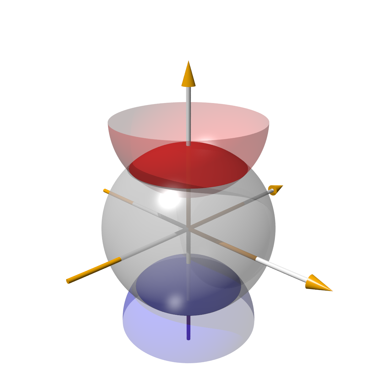
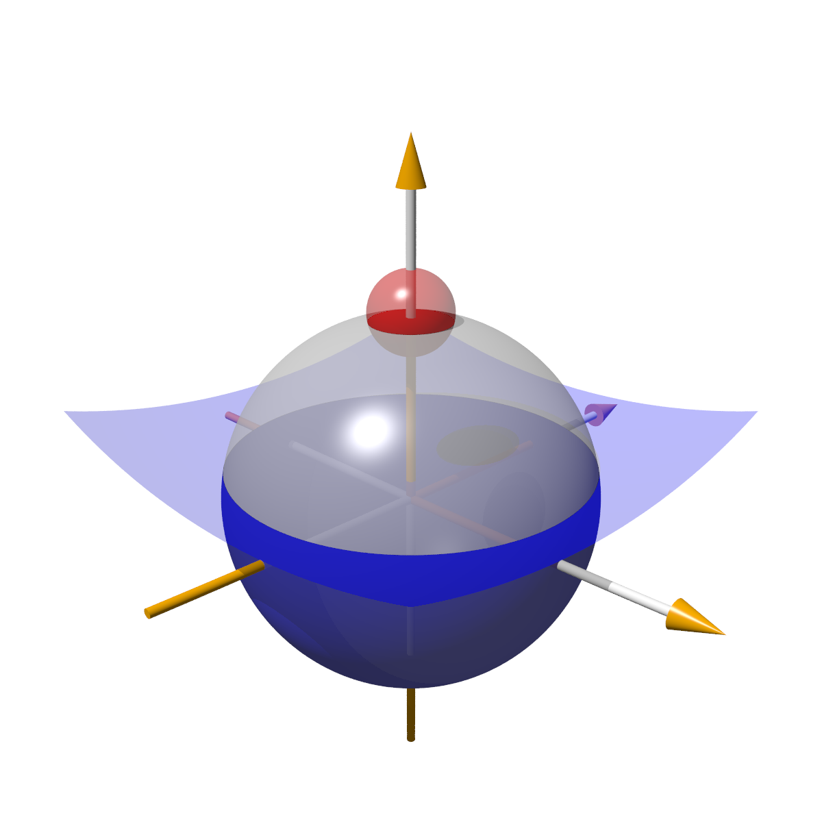
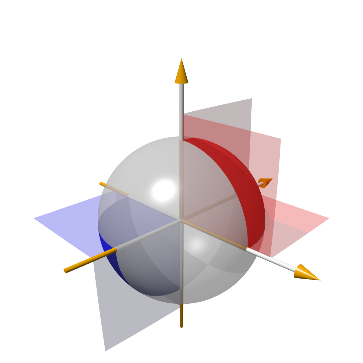
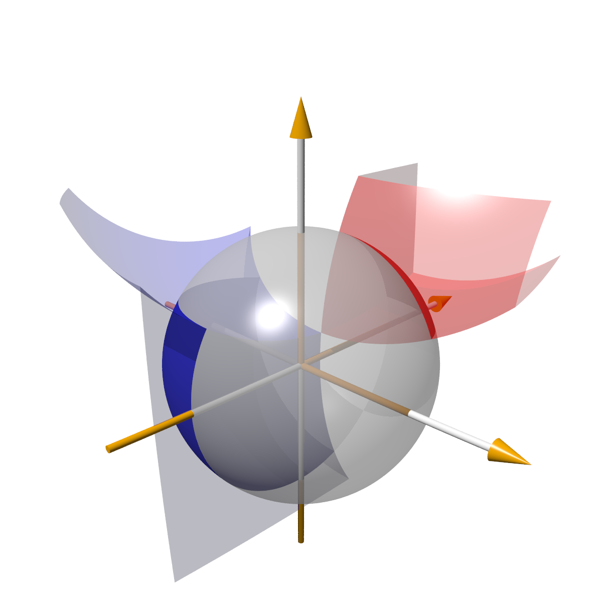
Figure 1: Geometries related by conformal transformations. The domain $\Omega$ is the sphere centered in the origin while the domains $\Omega_{i}$ are the the ones intersecting $\Omega$ which have, when necessary, been trimmed to fit the image. The domains $\omega_{i}$ are the the darker portions of $\Omega$. Panel $a$ refers to the cap geometry ($i$) with $\theta=0.45\pi/2$ and when it subject to transformation VIII in table 1 it is mapped onto the geometry shown in panel $b$. Please note that the sphere $\Omega_{2}$ gets mapped onto the exterior of a sphere under the action of the conformal transformation. Panel $c$ is the octant geometry ($ii$) and when acted on with transformation V in table 1 it is mapped onto the geometry shown in panel $d$.

By use of conformal transformations it is easy to see that the crossing probability will depend only on one anharmonic ratio $\alpha$. $\alpha$ is easily evaluated by mapping the surface of the sphere by a stereographic projection onto the (extended) plane and having the caps $\omega_{1}$ and $\omega_{2}$ mapped onto two circles with center in the origin ($z_{1}$) and the point at infinity ($z_{4}$). Scale invariance allows us now to set the radius of $\omega^{\prime}_{1}$ to be one ($z_{2}$). The only free parameter left is the radius of $\omega^{\prime}_{2}$ which we call $z_{3}$. We define the $\alpha$ to be the anharmonic ratio

$$\alpha=\frac{(z_{2}-z_{1})(z_{4}-z_{3})}{(z_{3}-z_{1})(z_{4}-z_{2})}=\tan^{2}\left(\frac{\theta}{2}\right).$$ (3)

written with its relation to the angle $\theta$. In this geometric setting conformal invariance implies that $\pi_{\times}$ depends only on $\alpha$.

$ii)$ The second geometry we will consider is the crossing probability among two spherical triangles on the unit sphere. The domains $\Omega_{1}$ and $\Omega_{2}$ will be chosen as the octants $x,y,z\geq 0$ and $x,y,z\leq 0$ respectively. The starting geometry is depicted in panel $c$ of figure 1. In panel $d$ of figure 1 we show the octant geometry when transformed with transformation V of Table 1.

III Percolation models

In order to test the invariance of crossing probabilities we will consider two types of percolation models, a discrete and a continuum one.

III.1 Discrete model

Take a (simple) cubic lattice $\mathbb{L}$ of lattice constant $\lambda$ i.e. $\mathbb{L}=\lambda(\mathbb{Z}^{3}+\{1/2,1/2,1/2\})$. The shift by the vector $\{1/2,1/2,1/2\}$ has been introduced in order to grant better scaling properties of our finite lattice realization. We have specialized to the site percolation problem. The sites will be filled with a probability $p$. Such a model has been one of the most widely studied among the percolation models in three spatial dimension. As known the percolation transition for $p=p_{c}$ where $p_{c}=0.31160768(15)$ xiao_2014 . As for the realization of the geometries introduced in Section II are concerned in the present model a point will be considered inside the domain if it belongs to $\mathbb{L}\cap\Omega$ while the points belonging to $\omega_{i}$ are the ones in $\mathbb{L}\cap(\Omega_{i}\setminus\Omega)$ having at least a nearest neighbor in the domain. In panel $a$ of figure 2 a 2d representation of the above model.

III.2 Continuum model

The continuum percolation model we have considered is the percolation of penetrable spheres mertens_2012 namely we extract the centers of the spheres of radius $\rho$ uniformly from the interior of $\Omega$ (Poisson point process). A sphere will belong to the $\omega_{i}$ if the distance of its center $c$ to $\Omega$ is less or equal than $\rho$ and $c$ is an element of $\Omega_{i}$. Please see panel $b$ of figure 2.

The existence of a percolating cluster depends on the so called filling factor $\eta$ defined as the mean number of objects $n$ times the ratio of the volume of the filling spheres to the total volume which in our case reads $\eta=n\rho^{3}$. The value $\eta_{c}$ for which the transition occurs is known from numerical experiments to be $\eta_{c}=0.34189(2)$ torquato_2012 and $\eta_{c}=0.341888(3)$ lorenz_2001 which is to date the most precise estimate of the critical filling.

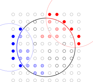
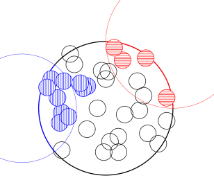
Figure 2: 2d cartoons of the percolation models we have considered in this work. Panel $a$ refers to the discrete percolation model whilst panel $b$ to the continuum one. The shaded circles in $a$ represent occupied sites, while in $b$ we depict the randomly occupied circles (spheres in our 3d model). The sites (in $a$) and circles (in $b$) with horizontal and vertical shadings (red and blue in color) represent cluster connected to the boundary domains $\omega_{1}$ and $\omega_{2}$ respectively. In both cases no cluster connecting $\omega_{1}$ and $\omega_{2}$ has been established.

IV Numerical Simulations

The discrete percolation experiments have been carried out on a simple cubic lattice $\lambda$ of decreasing lattice spacing, namely $1/\lambda=8,16,32,64,128$ in order to perform a scaling analysis. We have employed the Newman-Ziff newman_2000 ; newman_2001 algorithm to calculate the crossing probability. We have thus obtained the crossing probability $\pi_{\times}(n)$ as the lattice is filled (incrementally) with $n$ sites. From the above probabilities at fixed filling we can reconstruct the crossing probability $\pi_{\times}(p)$ in terms of any occupation probability $p$ via the following binomial convolution:

$$\pi_{\times}(p)=\sum_{n=0}^{N}\pi_{\times}(n)p^{n}(1-p)^{N-n}\binom{N}{n}$$ (4)

For the continuum percolation experiments we used spheres of radius $\rho$. We have considered the sizes of $\rho$ to be$1/\rho=2^{3},2^{3.5},2^{4},\ldots,2^{6.5},2^{7}$ with centers extracted uniformly from the volume under consideration.

In this case we resorted to the continuum version of the Newman-Ziff algorithm detailed in mertens_2012 . In this case the measurement of crossing probabilities with a given number $n$ of spheres $\pi_{\times}(n)$ allows to obtain the crossing probability for any filling factor $\eta$ by a poissonian convolution:

$$\pi_{\times}(\eta)=e^{n/\rho^{3}}\sum_{n=0}^{\infty}\pi_{\times}(n)\frac{(n/\rho^{3})^{n}}{n!}$$ (5)

The number of realizations used for our simulation consists of up to $10^{7}$ samples allowing us to obtain the desired statistical uncertainties.

For the random number generation we resorted to the, well tested for percolation simulations lee_2007 ; lee_2008 , Mersenne twister MT19937 by Matsumoto and Nishimura matsumoto_1998 .

V Results

V.1 Site percolation

In figure 3 (left panel) we depict the crossing probability as a function of the inverse lattice spacing for the cap geometry for some of the values of $\theta$ considered and for the octant geometry. These have been obtained by setting the occupation probability $p$ to the best known value $p_{c}=0.31160768(15)$ xiao_2014 .

As we can see groups of curves corresponding to the geometries related by a conformal transformation converge to the same value as the lattice realization becomes finer. Among the various mapped geometries we observe that VIII and IX are the ones differing the most from the others. This is to be expected since they are subject to more severe deformation such that one of the caps becomes very small (cfr. panel $b$ of Figure 1 referring to a geometry obtained by applying transformation VIII). When this happens even the finest simulated finite lattice realizations have stronger finite size effects.

In order to quantitatively assess the convergence to the same value in 3 (right panel) we plot the variance of $\pi_{\times}$ for the nine geometries considered for different values of $\theta$ which decay to zero, signalling the presence of the conformal symmetry in the thermodynamic limit.

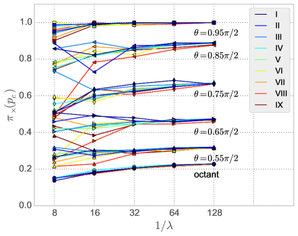
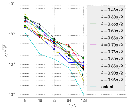
Figure 3: (Left panel) Crossing probabilities at $p_{c}$ as a function of the inverse lattice spacing $1/\lambda$. The different colors refer to geometries obtained by applying the transformations in table 1. The distinct bunches of curves refer to different values of $\theta$ and for the octant geometry. Statistical errors are smaller than the symbols. (Right panel) Variance of the crossing probabilities as a function of the system size for different values of $\theta$. The lines are just guide to the eyes.

By extrapolating these finite size results to the thermodynamic limit allows us to obtain a numerical estimate of the crossing probabilities for any two spherical cap on the sphere. The crossing probability in terms of the anharmonic ratio $\alpha$ is depicted in 4. In this figure we also plot the function

$$\tilde{\pi}_{\times}(\alpha)=\tanh\left(\tan\frac{\alpha\pi}{2}\right)$$ (6)

which appears to describe very well the values extrapolated in the thermodynamic limit. Indeed fitting the extrapolated values the function $\tanh\left(a\tan\frac{\alpha\pi}{2}\right)$ with $a$ free parameter gives a value of $a=0.989(6)$ very close to 1.

The function $\pi_{\times}$ we have numerically estimated and for which we have given an analytic approximation $\tilde{\pi}_{\times}(\alpha)$ is somewhat analogous to the Cardy’s formula cardy_1994 although in the two dimensional case, due to Riemann mapping theorem, all of the crossing probabilities among two distinct segment on the boundary of a connected domain can be obtained by this formula. In the three dimensional case instead the knowledge of the function plotted in 4 allows us to calculate the crossing probability among two arbitrary spherical caps on the surface of a sphere.

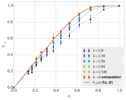
Figure 4: Crossing function for two spherical caps on a sphere in term of the anharmonic ratio $\alpha$ (defined in 3). The different curves refer to different system sizes, and to the extrapolation to the infinite size system. The dotted lines are just guide to the eyes. The continuous line refers to the function $\tilde{\pi}(\alpha)$ defined in Equation (6).

V.2 Continuum percolation

In contrast to the discrete model the continuum one has the added benefit of having a continuously tunable parameter $\rho$. Moreover as we lower $\rho$ the various crossing probabilities approach the thermodynamic limit in a much smoother way. In 5 we plot the crossing probability as function of the filling fraction for decreasing filling sphere radii for $\theta=0.75\pi/2$ for the configuration I. These curves clearly develop a steep profile as we approach the thermodynamic limit as shown in panel $a$ of Figure 5. We can use them to obtain reliable estimates of the critical filling fraction. In fact, by defining a size dependent $\eta_{c}(\rho)$ (the so called cell-to-cell estimator reynolds_1980 ) as the value for which the curves meet:

$$\pi_{\times}^{\rho}(\eta_{c}(\rho))=\pi_{\times}^{\rho/2}(\eta_{c}(\rho))$$ (7)

we can easily obtain an estimate for $\eta_{c}$. This analysis, shown in panel $b$ of Figure 5, with the $\theta=0.65\pi/2$ cap geometry I leads us to estimate the critical $\eta$ as $\eta_{c}=0.341935(8)$. We have chosen the value $\theta=0.65\pi/2$ and the configuration I since, among the many geometries we have simulated, it represents “best” the thermodynamic limit for it has the domains $\omega_{1}$ and $\omega_{2}$ of the same size and the ratio of sum the total area of the patches $\omega_{i}$ and the remaining surface is closest to 1. This estimate has to be compare with the ones available in literature torquato_2012 and lorenz_2001 which provide values of $\eta_{c}=0.34189(2)$ and $\eta_{c}=0.341888(3)$ respectively. Those results were obtained with growth algorithms on large systems. In our simulation the lowest value of $\theta$ ($\theta=0.45\pi/2$) simulated cap geometry resembles somehow the study of percolating clusters connecting two sides of a cube since the ratio of patches area to open surface area is closest to $1/2$. Performing the analysis on this configuration we obtain a value of $\eta_{c}=0.34190(1)$ which is consistent with the above cited values, showing how the determination of $\eta_{c}$ sensibly depends on the geometry for the sizes we have examined. We will rely on our “best” determined estimate $\eta_{c}=0.341935(8)$ for the subsequent analysis but we anticipate that the final results will not be crucially affected by the choice of $\eta_{c}$.

The convergence to the same value for $\pi_{\times}$ for geometries related by a conformal transformation can seen in the left panel of Figure 6 which is the continuum analogue of the left panel in Figure 3. The curves for $\pi_{\times}$ nicely converge to the thermodynamic limit, since the effects from discretization are not present; on the other hand finite size effects are stronger, for the range of $\rho$ simulated, since their distance is in general bigger than the curves for the discrete systems. Once again we observe that configurations generated with VIII and IX transformations are more distant from the other curves confirming that, for the same value of $\rho$, they are more far from the thermodynamic limit.

The good behavior of the finite realizations allows to have an independent extrapolation for each configuration. This is shown in the right panel of Figure 6 where the extrapolated values of the crossing probabilities are shown for the set of conformal transformations examined together with the mean over the various configurations. This confirms the onset of conformal invariance even for a continuum percolation model

For comparison we also report, in the left panel of figure 7, the same analysis performed with the critical filling reported in lorenz_2001 for the cap geometry with $\theta=0.45\pi/2$. As we can see in both cases the different transformed geometries give the same value within $1.5\sigma$ so they are consistent with each other. This proves that within our error, both values of $\eta_{c}$ give the same value for the crossing probability in domains related by a conformal mapping although the value of $\pi_{\times}$ depends on the chosen $\eta_{c}$. Similar findings are obtained for the other values of $\theta$ examined and for the octant geometry.

The function $\pi(\alpha)$ (6), introduced in the previous section, ruling the crossing probability among two caps in on the sphere, is depicted in the left panel of 7. As we can see the values are consistent, within errors, with the function obtained from the site percolation model. This provides an evidence of universality of $\pi_{\times}$ in percolation. Moreover if we compare it with the analytic function $\tilde{\pi}_{\times}$ 6 proposed in the previous section we find an excellent agreement with the data obtained setting $\eta_{c}$ to the value provided in lorenz_2001 while if we choose our best estimate of $\eta_{c}$ we have a less faithful representation of the numerical data by 6. If we try to fit the above data with the more general function $\tanh\left(a\tan\frac{\alpha\pi}{2}\right)$ indeed we obtain the estimates of $a=1.022(6)$ for $\eta_{c}=0.341935$ (our best value) and $a=1.005(5)$ for $\eta_{c}=0.341888$ (given in lorenz_2001 ).

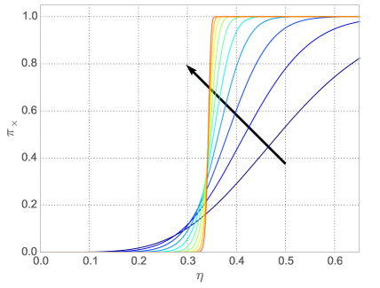
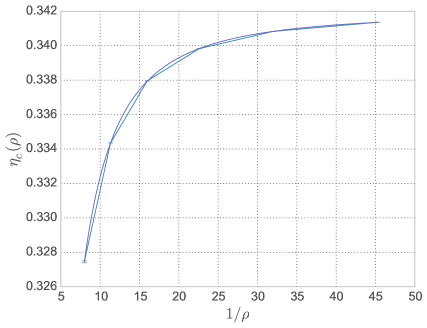
Figure 5: (Left panel)Crossing probability as a function of the filling factor for the cap geometry with $\theta=0.65\pi/2$. The different lines refer to the filling spheres of increasing radius $1/\rho=2^{2},2^{2.5},\ldots,2^{6.5}$ in the direction of the arrow. The errors are not showed being smaller than $2.5\cdot 10^{-4}$ for all the points i.e. smaller than the lines size. (Right panel) Finite size estimations of $\eta_{c}(\rho)$ as a function of $1/\rho$. The continuous line is the best fitting function $0.341935-0.687988\rho^{1.85758}$. The two lowest values of $1/\rho=2^{2},2^{2.5}$ have been excluded from the fit.

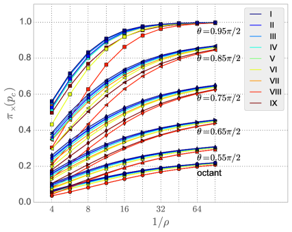
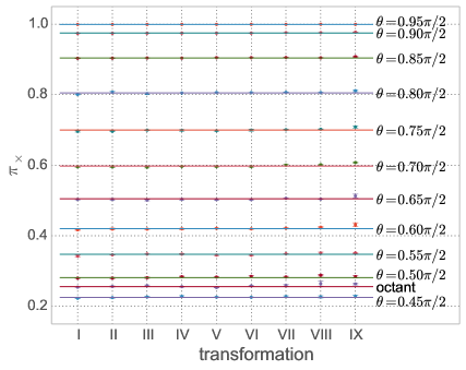
Figure 6: (Left panel) Crossing probabilities $\pi_{\times}(L)$ of conformally equivalent cap geometries and octant geometry as the radius $\rho$ of the filling spheres is reduced, cfr. left panel of Figure 3. The crossing probabilies are calculated at $\eta=\eta_{c}$. (Right panel) Extrapolated values of $\pi_{\times}$ in the thermodynamic limit for the caps and octant geometry with for the different conformal transformations considered 1.

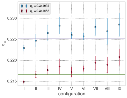
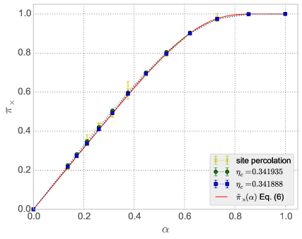
Figure 7: (Left panel) Extrapolated values of $\pi_{\times}$ in the thermodynamic limit for the cap geometry with $\theta=0.45\pi/2$ for the different conformal transformations considered 1. The two curves refer to the values obtained setting $\eta$ to our best estimated value (upper curve) and the value. given in lorenz_2001 . (Right panel) Comparison between the values extrapolated at infinity for the site percolation model and the continuum percolation model with the two estimates for $\eta_{c}$ as a function of the anharmonic ratio $\alpha$ (3). We also report the function $\tilde{\pi}(\alpha)$ defined in (6).

VI Conclusions

By means of numerical experiments we have assessed the invariance under conformal transformation of selected both discrete and continuous percolation problems in three dimensions at criticality in bounded domains. We also proposed an analytical function approximating with very good accuracy the crossing probability among two arbitrary spherical caps on a sphere.

We hope that our work can stimulate from one side a study of percolation by conformal bootstrap techniques and from the other further investigation of symmetries of general percolation models. Future work in our opinion interesting will entail the analysis of bulk observables and the study of different statistical mechanics models such as $O(N)$ and Potts models.

Note added: During final stage of this work the authors noticed on arXiv a very recent and very interesting paper on the numerical investigation of Ising model on spherical domains with the help of the insight gained from the conformal bootstrap analysis of the model penedones_2015 for the finite size scaling analysis of correlators. The work penedones_2015 concentrates on observables lying in the bulk of a three dimensional Ising model. It would be interesting to extend the analysis of penedones_2015 to observables living on the boundary. For the percolation the corresponding analysis of operators living either in the bulk or in the boundary of the pertinent three dimensional boundary CFT has, to the best of our knowledge, not been derived.

Acknowledgements: We acknowledge useful discussions with Defenu N and Delfino G. The authors benefitted from computational resources from the Iscra C project COSY3D at CINECA Bologna Italy.

References

- (1) Mussardo G Statistical Field Theory: an Introduction to Exactly Solved Models in Statistical Physics 2010 (Oxford: Oxford University Press)
- (2) Di Francesco P, Mathieu P, and Sénéchal D Conformal Field Theory 1997 (New York: Springer)
- (3) Riva V and Cardy J Phys. Lett. B 2005 622 339
- (4) Witten E Adv. Theor. Math. Phys. 1998 2 253
- (5) Heemskerk I, Penedones J, Polchinski J and Sully J 2009 JHEP 09 079
- (6) Dorigoni D and Rychkov S arXiv:0910.1087
- (7) Rajabpour M JHEP 2011 06 076
- (8) Guida R and Zinn-Justin J 1998 J. Phys. A 31 8103
-
(9)
El-Showk S, Paulos M F, Poland D, Rychkov S, Simmons-Duffin D and Vichi A 2012 Phys. Rev. D 86 025022
El-Showk S, Paulos M F, Poland D, Rychkov S, Simmons-Duffin D and Vichi A 2014 J. Stat. Phys. 157 869 - (10) El-Showk S, Paulos M F, Poland D, Rychkov S, Simmons-Duffin D and Vichi A 2014 Phys. Rev. Lett. 112 141601
- (11) Polyakov A M 1970 JETP Lett. 12 381
- (12) Polchinski J 1988 Nucl. Phys. B 303 226
- (13) Seiberg N and Witten E 1994 Nucl. Phys. B 431 484
- (14) Luty M A, Polchinski J and Rattazzi R 2013 JHEP 1301 152
- (15) Fortin J-F, Grinstein B and Stergiou A 2013 JHEP 1301 184
- (16) Delamotte B, Tissier M and Wschebor N arXiv:1501.01776
- (17) Cardy J 1994 J. Phys. A 25 L201
- (18) Langlands R, Pouliot P and Saint-Aubin Y 1994 Bull. Am. Math. Soc. 30 1
- (19) Cardy J L 1985 J. Phys. A 18 L757.
- (20) Deng Y and Blöte H W J 2002 Phys. Rev. Lett. 88 190602
- (21) Deng Y and Blöte H W J 2003 Phys. Rev. E 67 066116
- (22) Deng Y and Blöte H W J 2004 Phys. Rev. E 69 066129
- (23) Janke W and Weigel M 2002 Comp. Phys. Comm. 147 382
- (24) Stauffer D and Aharony A Introduction to Percolation Theory 1992 (London: Taylor & Francis)
- (25) Saberi A A 2015 Phys. Rep. 578 1
- (26) Aizenman M and Barsky D J 1987 Commun. Math. Phys. 108 489
- (27) Smirnov S 2006 Proc. Int. Congr. Math. 2 1421
- (28) Schramm O 2001 Elec. Comm. in Probab. 6 115
- (29) Newman M E J and Ziff R M 2000 Phys. Rev. Lett. 85 4104
- (30) Newman M E J and Ziff R M 2001 Phys. Rev. E 64 016706
- (31) Watts G M T 1996 J. Phys. A 29 L363
- (32) Simmons J J H 2013 J. Phys. A: Math. Theor. 46 494015
- (33) Škvor J, Nezbeda I, Brovchenko I and Oleinikova A 2007 Phys. Rev. Lett. 99 127801
- (34) Lorenz C D and Ziff R M 1998 J. Phys. A: Math. Gen. 31 8147
- (35) Diehl H W 1998 Int. J. Mod. Phys. B 11 3503
- (36) Pleimling M 2004 J. Phys. A 37 R79
- (37) Diehl H W and Lam P M 1989 Z. Phys. B - Condensed Matter 74 395
- (38) Xiao X, Wang J, Lv J-P and Deng Y 2014 Frontiers of Physics 9 113
- (39) Mertens S and Moore C 2012 Phys. Rev. E 86 061109
- (40) Torquato S and Jiao Y 2012 J. Chem. Phys. 137 074106
- (41) Lorenz C D and Ziff R M 2001 J. Chem. Phys. 114 3659
- (42) Lee M J 2007 Phys. Rev. E 76 027702
- (43) Lee M J 2008 Phys. Rev. E 78 031131
- (44) Matsumoto M and Nishimura T 1998 ACM Trans. Mod. Comp. Sim. 8 3
- (45) Reynolds P J, Stanley H E and Klein W 1980 Phys. Rev. B 21 1223
- (46) Cosme C, Viana Parente Lopes J M and Penedones J arXiv:1503.02011