Properties of weak lensing clusters detected on Hyper Suprime-Cam’s 2.3 deg² field

Abstract

We present properties of moderately massive clusters of galaxies detected by the newly developed Hyper Suprime-Cam on the Subaru telescope using weak gravitational lensing. Eight peaks exceeding a S/N ratio of 4.5 are identified on the convergence S/N map of a 2.3 deg² field observed during the early commissioning phase of the camera. Multi-color photometric data is used to generate optically selected clusters using the CAMIRA algorithm. The optical cluster positions were correlated with the peak positions from the convergence map. All eight significant peaks have optical counterparts. The velocity dispersion of clusters are evaluated by adopting the Singular Isothemal Sphere (SIS) fit to the tangential shear profiles, yielding virial mass estimates, $M_{500_{c}}$, of the clusters which range from 2.7$\times$10¹³ to 4.4$\times$10${}^{14}\;M_{\odot}$. The number of peaks is considerably larger than the average number expected from $\Lambda$CDM cosmology but this is not extremely unlikely if one takes the large sample variance in the small field into account. We could, however, safely argue that the peak count strongly favours the recent Planck result suggesting high $\sigma_{8}$ value of 0.83. The ratio of stellar mass to the dark matter halo mass shows a clear decline as the halo mass increases. If the gas mass fraction, $f_{g}$, in halos is universal, as has been suggested in the literature, the observed baryon mass in stars and gas shows a possible deficit compared with the total baryon density estimated from the baryon oscillation peaks in anisotropy of the cosmic microwave background.

1. Introduction

Clusters of galaxies are the largest gravitationally bound systems in the universe and have been useful cosmological probes to learn about the geometry and structure of the universe. X-ray observations have, to date, provided the most efficient way to collect samples of clusters. Cluster catalogs compiled from the ROSAT All-Sky Survey (Voges et al., 1999) have often been used in combination with follow-up observations by XMM/Chandra to give rigorous cosmological constraints. Based on a sample of 238 clusters with redshifts ranging from 0 to 0.5, Mantz et al. (2010) present constraints on the density parameters ($\Omega_{\rm M}$ and $\sigma_{8}$) from cluster abundance and on the dark energy parameters ($\Omega_{\rm X}$ and $w_{0}$) from the redshift evolution of that abundance. The mass fraction of host gas, $f_{\rm gas}$, measured at large radii in the most massive halos is also used to as a cosmological probe, as it provides a direct measure of the luminosity distance under the assumption of the universality of the gas fraction in massive halos; it is expected to scale as $f_{\rm gas}(z)\propto d(z)^{3/2}$, and is sensitive enough to give a level of constraint on the parameters comparable to those from other methods (Allen et al., 2008). So far, no significant departure from $\Lambda$CDM model is reported. The eROSITA satellite is scheduled to launch in 2016 and is expected to collect yet more clusters in a more distant redshift range, and is expected to obtain more stringent constraints (Predehl et al., 2010) .

In the mean time, the clusters themselves draw astronomers’ interests as a site of galaxy formation and galaxy-galaxy interactions. Galaxy formation is a process which is accompanied by the conversion of baryons into stars in a dark matter halo; the star formation efficiency is critically dependent on the ability of the gas to cool. In a less massive dark matter halo, the gas is easily reheated and swept out from the center by feedback processes such as supernova explosions. In a massive halo, the cooling time becomes longer as the halo mass becomes larger and the virial gas temperature higher, and galaxy formation is expected to be suppressed. It is also argued that AGN could provide an efficient star-formation suppression feedback mechanism in the higher mass range. These considerations indicate that there is an optimal halo mass where star formation is most effective around $10^{12}\;M_{\odot}$ and where the stellar mass to halo mass ratio should peak. Statistical estimate based on the abundance matching technique generally agree with these naive expectations. (Behroozi et al., 2010).

In terms of individual halos, we now have accumulating observational evidences that the star formation efficiency actually drops as the host dark matter halo mass increases in the group to cluster scale, $>10^{13}\;M_{\odot}$, (Lin et al., 2003; Gonzalez et al., 2007; Andreon, 2010; Zehavi et al., 2012; Leauthaud et al., 2012; Gonzalez et al., 2013). These observational efforts are also motivated by the desire to measure the total baryon mass (gas and stars) to dark matter ratio and to compare with the universal baryon to dark matter density ratio measured from the anisotropy of the cosmic microwave background. This is, of course, related to the interesting ”missing baryon problem” (Fukugita et al., 1998; Fukugita, 2003), and quantitative measurements are important.

However, the discrepancy among the observations are quite large so far. On the one hand, using 12 galaxy clusters at redshifts around 0.1 with $M=1\sim 5\times 10^{14}\;M_{\odot}$, Gonzalez et al. (2013) argue that the difference between the universal value and cluster baryon fractions is less than the systematic uncertainties associated with the mass determinations. On the other hand, Leauthaud et al. (2012) insists clear shortfall based on the observation of X-ray groups with $1\sim 7\times 10^{13}\;M_{\odot}$, in COSMOS field.

This confusion may arise partly from the variety of halo mass measurement techniques. Gonzalez et al. (2013) estimate the halo mass from the X-ray temperature using the usual virial scaling relation in which they assume the X-ray gas is in hydrodynamic equilibrium. The dynamical method adopted in Andreon (2010) assumes that the system is virialized, which many not be true in the outer region of the clusters. Leauthaud et al. (2012) estimates the mass primarily from X-ray luminosity although this is calibrated by weak lensing. The chosen methods work best in different mass ranges, and their systematics almost certainly exist and are almost certainly different from technique to technique. Wu et al. (2015) reported that the gas fraction is anti-correlated with stellar mass fraction in their simulation. This could shift the ratio of the stellar mass over the halo mass which introduces another complexity in the studies based on the optically or X-ray selected clusters.

In this paper, we employ new approach to sample clusters and measure the halo mass directly by weak lensing with the fewest assumptions about the dynamical state of the cluster. As a part of the commissioning run on the Subaru telescope of the newly developed Hyper Suprime-Cam (Miyazaki et al., 2012) camera, we observed a 2.3 deg² field in i-band. We use these observations to locate massive dark matter halos directly via weak lensing by means of the derived convergence map. A deep multi-color catalog is used to generate an optically selected cluster catalog with estimated redshifts using the novel CAMIRA algorithm (Oguri, 2014). This optical catalog is then correlated with the list of peaks in the convergence map. These peaks, if not coincident with optically selected clusters, can be spurious, generated by noise, can correspond to chance coincidences of less massive halos along the line of sight, or can corresponds to real clusters with very high mass-to-light ratio.

We chose the Deep Lens Survey (DLS) Field (Wittman et al., 2002) for this investigation, for which a deep multi-color galaxy catalog is publicly available, to generate the optical cluster catalog. Based on the shear selected cluster catalogs combined with the luminosity based catalog, we determine the cluster number count and the redshift distribution over a wide contiguous area over which observational systematic errors can be expected to be minimized, since the data are taken almost simultaneously over the whole field with an instrument with a wide field and relatively uniform Point Spread Function (PSF). We then determine the stellar mass fraction of individual shear selected clusters. The individual halo mass, estimated directly through lensing, ranges nicely between the samples of Leauthaud et al. (2012) and Gonzalez et al. (2013).

Not all the observing facilities allow this approach. In order to locate the individual dark matter halos, a high resolution surface mass density map is necessary, which requires a sufficient number density of faint background galaxies whose shapes are measured with the necessary accuracy. With a much wider field of view (roughly ten times the area) than the original Suprime-Cam (Miyazaki et al., 2002b), the 1.5 degree Hyper Suprime-Cam (HSC) field on the 8.2 m Subaru telescope has a crucial advantage for a weak lensing survey. We have an approved plan to carry out a three layer legacy survey using Hyper Suprime-Cam (Miyazaki et al., 2013). Based on the pilot observations presented here, we attempt to demonstrate the prospects of the power of the legacy survey.

2. Data Analysis

2.1. Data set

DLS Field 2 was observed on February 4th, 2013 Hawaii time. As is shown in Table1, two pointing centers are chosen whose angular distance is 0.75 degree apart. Because the field of view of HSC is 1.5 degree, we have substantial overlap between two pointings. The exposure time is either 300 sec (9 exposures on south, 8 exposures on north) or 150 sec (4 exposures on north), and the total exposure time of south and north pointing is 2700 sec and 3000 sec, respectively. A circular dithering pattern of radius 2 arcmin is adopted around each pointing center to fill the gap of CCDs. The position angle is increased by 72$\sim$90 degree between exposures.

Table 1Exposure information

Field	Filter	J2000	Texp [sec]	Med. Seeing [”]
South	HSC-i	(139.50, 30.00)	2700	0.58
North	HSC-i	(139.50, 30.75)	3000	0.57

FWHM map (a) and ellipticity whisker map (b) of one of the exposure on the south (200 second). On the right, dash line shows the tilt axis estimated from the ellipticity pattern. The median FWHM and the ellipticity over the field is 0”.58 and 4.6 %, respectively.

The median stellar image (PSF) size of each exposure varied between 0”.52 and 0”.63 and the overall average was 0”.58. Fig. 2.1(a) shows the map of the PSF size over the field of view (FOV). The non-uniformity is visible and we observe a hump of 0”.65 in lower left bottom and minimum of 0”.51 at slightly upper-right from the center. This is not expected from the design and the tolerance analysis and suggests that at this early stage the collimation of the optical system was insufficiently accurate.

To investigate this, we evaluate spatial variation of the ellipticities of stars, $\{e_{1},e_{2}\}$, which is defined as

$$\ooalign{\hfil/\hfil\crcr$e$}=\{e1,e2\}=\{I_{11}-I_{22},2I_{12}\}/\left(I_{11}+I_{22}+2\sqrt{I_{11}I_{22}-I_{12}^{2}}\right)$$ (1)

where $I_{ij}$ is Gaussian-weighted quadrupole moment of the surface brightness distribution.

Fig. 2.1(b) shows a whisker plot where we present the position angle of the ellipse with a bar whose length is proportional to the ellipticity. We find a typical pattern of astigmatism generated by the tilt of the camera optics with respect to the optical axis of the primary mirror. In this case, the camera is tilted around the axis shown in the figure as a dashed line. From the start to the end of this observation, the instrument rotator (InR) rotated by 68 degrees. The fix pattern seen on the FWHM and whisker plot co-rotated as the InR rotated which supports of our interpretation of the non-uniformity of the PSF.

Recall that these test images were taken in the very first engineering run of the full FOV, we were trying to establish the way to measure the collimation error. Thus these particular images were taken under rather poor alignment conditions. The median ellipticity over the FOV is roughly 5 % (Fig. 2.1(b)) which is slightly larger than typical 3$\sim$4 % raw ellipticity seen on Suprime-Cam images. (Miyazaki et al. (2007) Fig.1). It is hard to determine the inclination angle from these data set alone but it is roughly a few arcmin level. By the time of this writing, we have established a way to measure the tilt and have implementered an auto-focus system, and we no longer see non-uniform patterns like this (Miyazaki et al., 2015).

2.2. Image Reduction and the galaxy catalog

HSC has 116 2k$\times$4k CCDs in total: 104 for imaging, in the central part of the field, and at the edges 4 CCDs for auto guiding and 8 CCDs for focus monitoring. We use the auto-guiding for the observations reported here. Each CCD has 2048$\times$4176 physical pixels (15$\mu$m: 0”.169 at the field center). The imaging area of each device consists of 4 512$\times$4176 stripes; each stripe is read through an independent output amplifier located on one side of one of the shorter edges. Each segment has an 8 pixel wide pre-scan and we add 16 pixels of over-scan along the serial register and 16 lines of over-scan along the parallel register.

We use the serial over-scan region for the zero reference of each amplifier (bias level). The median value of the pixel data on one row is used for the bias level for pixels on that row and subtracted. Non-physical reference pixels are trimmed from each segment and the segments are tiled together to reconstruct the original 2048$\times$4176 image. We then divide the image by a flat field image that is generated from an average of dome flatfield images (typically 10 images). Sky level is evaluated on by medianing on a mesh whose element size is 256$\times$256 pixels and fitted with 2-D polynomial. This is subtracted from the image. This reduced CCD image file is one unit of the data source for the shape measurement (Section2.3).

The basic image analysis pipeline is developed through a collaboration of multiple institutions including Princeton University, Kavli IPMU and NAOJ. It is based on a customized version of the “LSST-stack” (Ivezić et al., 2008; Axelrod et al., 2010), a software suite being developed for the LSST project. Object detection is made on each CCD image. The PSF on a CCD is modeled as a function of the CCD pixel coordinates, and can be reconstructed accurately at any pixel position. This is used in the subsequent morphological classification process which tags star/galaxy flags as well as flagging cosmic rays. The flags are stored on the mask layer in an output FITS file.

The star catalog is correlated with an external catalog (SDSS-DR8) for each CCD to perform photometric and astrometric calibration, by using a cross-matching alogorithm of astrometry.net (Lang et al., 2010). The SDSS magnitudes are transformed into the very similar HSC bands for photomteric zeropoints, and the astrometry.net is applied to the SDSS coordinates to determine the world coordinated system of each CCD.

The angular displacement of the control stars among exposures in the mosaic-stack process. The position averaged over the exposures is the reference (a) whereas the position in the external catalog is the reference (b).

Because the number of stars on each CCD matched with astrometric catalog is limited ($\leq$ 50), the accuracy of the astrometric solution is not sufficient for the later image stacking process. In order to minimize the mosaic-stacking error, the residual of i-th control stars on a e-th exposure from a reference frame, $(\Delta x_{ie},\Delta y_{ie})$, is parameterized as a polynomial function of the field position, $(x,y)$, as

$$\Delta x_{ie}=\sum^{N}_{l=0}\sum^{l}_{m=0}a_{lme}x^{l-m}y^{m}\;\;\;\;\Delta y_{ie}=\sum^{N}_{l=0}\sum^{l}_{m=0}b_{lme}x^{l-m}y^{m}$$ (2)

This is a ’Jelly CCD’ approach adopted in Miyazaki et al. (2007), which is is particularly important for HSC where we have significant non-axisymmetric distortion pattern caused by the larger index mismatch of the glass used for the atmospheric dispersion corrector (Miyazaki et al., 2015). The implementation on the HSC pipeline is more sophisticated. Rather than dealing with the polynomial as a function of the pixel coordinate as above, the SIP convention (TAN-SIP) of World Coordinate System (WCS) is employed to allow the Jelly warp of the CCDs. A point on Fig. 2.2 (a) shows the displacement of the astrometric position of the the control star with respect to the position on the first exposure, thus the scatter presents a measure of the mosaic-stacking error. This internal error is as low as 6 to 7 mili-arcsec (mas). A point on Fig. 2.2 (b) shows the displacement from the external catalog and the scatter is larger (abut 60 mas) which we suppose is partly due to the astrometric error of the external catalog itself. The peak position of the distribution in (b) has no offset from the origin which indicates that there is no systematic error on astrometric solution. The composition of the internal (a) and external (b) error gives a estimate of the total astrometric error of $\sim$ 20 mas in this analysis. Once the global solution over the multi exposures are obtained, the WCS of each CCD image is refreshed for further usage in the lensing analysis.

Handling a entire mosaic-stacked image all at once is usually not practical. We divide the image into a set of patches whose size is $4200\times 4200$ pixel. In order to take care of objects fallen on the boundary of the patches, we implement 100 pixel overlap between neighboring patches. The patch is a unit of the following mosaic-stack operation and the object detection on the co-added image. We then combine the object catalogs of all paces into a single catalog by removing the objects detected multiple times within the overlapped region. From the combined catalog, we extract the coordinate of moderately bright stars (22.0 $<$ HSC-i $<$ 24.5) for star catalog and the coordinate and the magnitude of galaxies. The star and the galaxy catalog as well as the image files with refined WCS of each CCDs (before the stack) are handed over to the next stage where we carry out the weak lensing shear estimate.

2.3. Galaxy shape measurements and the shear estimates

In the Suprime-Cam weak lensing survey (Miyazaki et al., 2002a, 2007), we employed rather traditional method where we measured the galaxy shapes on the fully reduced mosaic-stacked CCD image. The PSF is not precisely round, nor is it of uniform size over the whole field. It is evaluated from star images over the whole field. (Eqn.1). Because the PSF varies over the field of view (Fig. 2.1(b)), the PSF ellipticities are represented as a polynomial function of the field position. Analysis on the mosaic-stacked image requires that the PSF pattern does not change much during the series of exposures and that the CCD boundary does not cause a discontinuity of the PSF variation. Otherwise, the PSF becomes too complicated to represent as a simple polynomial function of the field position, and could cause systematic error in the galaxy shape measurement. In the case of the Suprime-Cam survey, we determined that the conditions were mostly met because one field was observed in a relatively short time span (40 minutes) with a small ($\sim$ 2 arcmin) dithering offset and we had a small CCD mosaic. However, in the planned HSC survey one field observation is split into several semesters to search for variables and the circular FOV requires relatively large (nearly a half of the FOV) dithering step. It is therefore not expected that this simple requirement will be met. Instead, the galaxy shapes will be evaluated on the pre-stacked image and then combined after that to reduce the statistical error. When the survey is underway, we will develop code to determine shapes and fluxes simultaneously from the constituent images, which is arguably the most statistically efficient use of the data.

For this early data, we have adopted Bayesian galaxy shape measurements implemented in the “lensfit” algorithm (Miller et al., 2007; Kitching et al., 2008) in this work. The PSF employed in the lensfit is not a simple elliptical but more empirical 32$\times$32 pixel postage stamp image. Each pixel value of the postage stamp is fitted independently on each exposure to a 2D-polynomial function of the sky-coordinate. lensfit also allows varying low order coefficients between CCDs to further minimize the residual on each CCD.

Galaxy shape measurement is made on the 40$\times$40 pixel postage stamp image of each galaxy. From a galaxy coordinate on the given catalog, the postage stamp image is trimmed from the un-warped original CCD image by using the WCS information. Usually, the galaxy is imaged on multiple exposures and multiple postage stamps are created for one galaxy. lensfit has two galaxy model components; de Vaucouleurs profile bulge and exponential disk. The center of the two models are assumed to be aligned. The ellipticity, the 1-D size, the normalization and the bulge-to-disk ratio are the parameters which model a galaxy. The postage stamp image of the model galaxy is convolved with the estimated PSF image at the galaxy position and the convolved image is compared with observed galaxy image to calculate the residual. By minimizing the residual, the best fit galaxy model and the ellipticity is estimated. In the fitting process, multiple exposures data are simultaneously fitted. Note that the galaxy position is a free parameter as well, and is marginalized by integrating under the cross-correlation function of the galaxy model and the data. Therefore, the astrometric error in the mosaic-stack process has limited impact on the error in the shape measurement. Note also that the observed image is not re-sampled nor warped onto the new coordinate in this process, which avoids the introduction of correlated noise mentioned in Hamana et al. (2008).

For PSF modeling, we employ 2nd order polynominals for the exposure wide fit and 1st order polynominal for the CCD term. Fig. 2.3 (a) shows the ellipticity whisker plot of one exposure that is calculated from the PSF model postage stamp and averaged in the grid to visually compare with the observed PSF shown in Fig. 2.1. Fig. 2.3 (b) shows the difference of the observed and modeled ellipticity. The residual is sufficiently small as $\sigma_{e}<1$ %.

Ellipticity whisker plot of modeled PSF (a) and the residual between the model and the observed data. The sigma of the scatter is 0.7 % and 0.6%, respectively in each component of the ellipticity.

In the following sections, we adopt galaxies brigher than $i=24.5$ for the mass map reconstruction. The rms sigma of the ellipticity of adopted galaxies is 0.41 and the galaxy number density is 20.9 /arcmin². In order to estimate the shear bias, we calculate mean ellipticities of galaxies used for the lensing analysis. The result is $(\left<e_{1}\right>,\left<e_{2}\right>)=(0.005,-0.004)$, which is sufficiently small for this study. However, the bias is not completely negligible for cosmic shear studies and further investigations about the origin will be necessary in the future.

2.4. Weak Lensing Convergence S/N map

The dimensionless surface mass density, the convergence $\kappa(\mbox{\boldmath$\theta$})$ is evaluated from the tangential shear as

$$\kappa(\mbox{\boldmath$\theta$})=\int d^{2}\phi\gamma_{t}(\mbox{\boldmath$\phi$}:\mbox{\boldmath$\theta$})Q(|\mbox{\boldmath$\phi$}|)$$ (3)

where $\gamma_{t}(\mbox{\boldmath$\phi$}:\mbox{\boldmath$\theta$})$ is the tangential component of the shear at postion $\phi$ relative to the point $\theta$ and $Q$ is the filter function. We adopt as a filter the truncated Gaussian

$$Q_{G}(\theta)=\frac{1}{\pi\theta^{2}}\left[1-\left(1+\frac{\theta^{2}}{\theta_{G}^{2}}\right)\exp{\left(-\frac{\theta^{2}}{\theta_{G}^{2}}\right)}\right],$$ (4)

for $\theta<\theta_{o}$ and $Q_{G}=0$ elsewhere (Hamana et al., 2012). We employ $\theta_{G}=1$ arcmin and $\theta_{o}=15$ arcmin, respectively.

We adopt 9$\times$9 arcsec grid cells and then calculate the convergence, $\kappa(\mbox{\boldmath$\theta$})$, on each grid using Eqn.(3) to obtain the $\kappa$ map. In order to estimate the noise of the $\kappa$ map, we randomized the orientations of the galaxies in the catalog and created a $\kappa_{noise}$ map. We repeated this randomization 100 times and computed the rms value at each grid point. Assuming the $\kappa$ error distribution is Gaussian, this rms represents the 1-$\sigma$ noise level, and thus the measured signal divided by the rms gives the signal-to-noise ratio (S/N) of the convergence map at that point.

Fig. 1 is the convergence S/N map so obtained. Wittman et al. (2006) showed a convergence map based on the DLS R-band imaging. We find general agreement with that map although the resolution of the our map is higher. Note, however, that the convergence map of Wittman et al. (2006) was generated in the middle of the survey and it did not employ the full depth image of DLS. They identifed two shear selected clusters on the map: DLSCL J0920.1+3029 (140.033, 30.498) and DLSCL J0916.0+2931 (139.000, 29.526) and we see the corresponding peaks on our map.

The former is a complex Abell 781 cluster region where at least four clusters have been identified so far from X-ray data and spectroscopic follow-up observations (Sehgal et al., 2008). In Fig. 2.4, we showed a close up view of the region. Crosses indicate the center of X-ray emissions (XMM) of the four clusters which is called “West”(z=0.4273), “Main”(z=0.302), “Middle”(z=0.291) and “East”(z=0.4265) respectively from west to east. We detect clear corespondent peaks in the latter three clusters. This demonstrates that the angular resolution of the weak lensing convergence map matches well with that of the XMM X-ray image.

We see two separate peaks on the convergence map at the “Main” cluster region and the mid-points of two peaks roughly coincides with the location of the X-ray emission center. The X-ray image is mostly round and no corresponding structure that is found on the lensing map is observed (Sehgal et al., 2008). Wittman et al. (2014) presented the convergence map on this A781 region based on the full depth DLS imaging but no structure is seen in the “Main” cluster in that map. The structure seen in Fig. 2.4 survived several reality checks in our analysis (change of the magnitude cut of galaxies and bootstrap re-sampling of galaxies) but obviously further observations are necessary to confirm the structure. If it is confirmed, it will provide another laboratory for testing the nature of dark matter following the famous “bullet cluster”. In fact, Sehgal et al. (2008) reported small extended sub-structure to the south-west of X-ray peak. Venturi et al. (2011) discovered possible radio relic in their deep radio map. These are indicative of a merger and already suggested that the “Main” is not simple system.

No significant peak is, however, found at the “West” position in Fig. 2.4. In fact, the lensing signal of the X-ray emitting cluster Abell 781 “West” has been a matter of debate. Motivated by the less significant detection on the original DLS map (Wittman et al., 2006), Cook & Dell’Antonio (2012) examined the region based on images independently obtained by the Orthogonal Parallel Transfer Imaging Camera on the WIYN 3.5 m telescope and Suprime-Cam. They concluded that no significant signal was observed on either of the convergence maps and argued that this example could pose a challenge to the usefulness of weak lensing for the calibration of lensing mass against other observable properties of clusters in observational cosmology. Wittman et al. (2014) claimed, however, that the strong “joint constraint” of Cook & Dell’Antonio (2012) was an artifact of incorrectly multiplying p-values. They re-visited the DLS data and tried to eliminate the contamination of foreground galaxies by adopting photometric redshift (photo-z) probability density weighting in the reconstruction of the convergence map. They suggested that the peak on the revised convergence map is still less significant (2.7 sigma level) but this does not strongly exclude the X-ray mass. We estimate the WL mass at X-ray position of the “West” cluster and the result is shown in Table 3. It is lower than what was obtained by Wittman et al. (2014) but 1-sigma error overlaps each other. Therefore, our result supports the summary by Wittman et al. (2014) saying that the mass of “West” cluster ($M_{200}$) ranges 1–3 $\times 10^{14}M_{\odot}$.

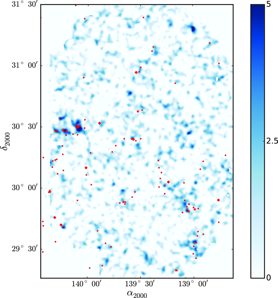
Figure 1.— Weak lensing convergence S/N map reconstructed from the shear catalog. The smoothing radius $\theta_{g}$ is 1 arcmin and galaxies brighter than 24.5 mag of HSC-i band are employed for the reconstruction. Red markers show the locations of clusters of galaxies registered on NASA/IPAC Extragalactic Database where the object type keyword ’GCluster’ was used to look up. The area below the declination of 31 degree is fully covered by Deep Lens Survey where Geller et al. (2010) carried out the spectroscopic campaign. Both Diamond and star markers show the location of SHELS clusters which match and un-match with he DLS lensing peaks, respectively (Geller et al., 2010).

Close up view of the convergence map (Fig. 1) at the Abell 781 multi-cluster region. Four cross marks are superimposed that indicate the location of the X-ray clusters observed by XMM: from west to east “West”, “Main”, “Middle” and “East”.

2.5. Cluster Searches based on the Multi-Color Catalog

The red symbols on Fig. 1 show the location of clusters of galaxies registered on NASA/IPAC Extragalactic database (NED). It is clear that the symbols tend to exist in the colored area (stronger lensing signal) and we see the general corespondence of the weak-lensing peaks and the cluster positions. Among them, the star and diamond symbols are SHELS clusters which are identified by Geller et al. (2010) employing uniform spectroscopic observation of a magnitude-limited (R ¡ 20.6) sample using HectoSpec. Geller et al. (2010) matched their clusters with the DLS lensing peaks; the star symbols show the matched clusters and the diamonds, un-matched.

In order to make an independent comparison between the light and mass on this region, we search for clusters using the DLS public photometric data with a method, the “Cluster finding algorithm based on Multiband Identification of Red-sequence gAlaxies” (CAMIRA), developed by Oguri (2014). CAMIRA makes use of the stellar population synthesis (SPS) models of Bruzual & Charlot (2003) to compute SEDs of red-sequence galaxies, estimates the likelihood of being cluster member galaxies for each redshift using $\chi^{2}$ of the SED fitting, constructs a three-dimensional richness map using a compensated spatial filter, and identifies cluster candidates from peaks of the richness map. For each cluster candidate, the brightest cluster galaxy candidate is identified based on stellar mass and location. Readers are referred to Oguri (2014) for more details of the algorithm and its performance studied in comparison with X-ray and gravitational lensing data.

We apply the CAMIRA algorithm to the DLS $BVRz$-band data. We apply a magnitude cut of $R<24.5$ to exclude galaxies with large photometric errors. In Oguri (2014), a number of spectroscopic galaxies in SDSS have been used to calibrate the SPS model. We adopt this SDSS calibration result, but we also add a constant 0.02 mag error quadratically to the model scatter, in order to accommodate the systematic offset of magnitude zeropoints and the difference in magnitude measurements between DLS and SDSS. We confirm that this SDSS-calibrated SPS model provides reasonable $\chi^{2}$ values when fitted to spectroscopic SDSS red-sequence galaxies in the DLS field. The cluster catalog contains, for each cluster, the cluster center based on the brightest cluster galaxy identification, the photometric redshift, and the richness. The redshft and richness ranges are restricted to $0.1<z<0.8$ and $N>10$, respectively. In addition, in this paper we also compute the total stellar mass by summing up weighted stellar mass estimates of individual galaxies; the weights are the “weight factors” $w_{\rm mem}$, which resemble the membership probability of each galaxy (see Oguri 2014). Stellar mass estimates of individual galaxies are obtained from the SPS model fitting in which we assume a Salpeter initial mass function.

We estimate the stellar mass only using optical data set which could cause the significant error in the estimation because of the limited band-pass. When we argue the cluster members in this work, however, we mainly deal with passvie galaxies whose stellar mass is expected to be easier to estimate compared with that of other general galaxies. In fact, Annunziatella et al. (2014) argued that the stellar mass of passive galaxies estimated from optical data agree well with what is estimated from optical and NIR data within 25 % if they adopt the template of passive galaxies in the calculation. Therefore we expect that our stellar mass estimates are not significantly biased by the absence of NIR data.

In Fig. 3.1, we show the positions of resultant optically selected clusters as open circles where the center of the clusters is defined as the position of the bright cluster galaxy (BCG). The redshift is color-coded as is presented on the side bar. The diameter of the circles is 3 arcmin.

3. Results and Discussions

3.1. Correlation of the Peaks on the Convergence Map and the Optically Selected Clusters

We have searched for peaks in the convergence map; the results are indicated on Fig. 3.1 as filled triangles (significant peaks of S/N ¿ 4.5) and filled squares (moderate peaks of 3.7 ¡ S/N ¡ 4.5). We then match the peaks with the centers of the optically selected clusters and count the coincidences as we vary the match tolerance. As is shown in Fig. 3.1, when we increase the tolerance from zero, the number of matches rises rapidly and reaches a plateau at about 1.5 arcmin. The displacement of the BCG from the cluster center (as defined by the X-ray emission center) can be as large as 0.5 Mpc/h (Oguri, 2014), which corresponds to $\sim$ 1.5 arcmin at the redshift of 0.7; the highest redshift in our sample. We would therefore expect to have to use a match tolerance of this order to recover real matches, and this is what we see; at approximately this tolerance we have recovered all the real matches and the number should plateau, as it does. The number of matches increases again slowly beyond $\sim$ 4 arcmin which we understand as accidental coincidences.

Table2 shows the list of our peaks sorted by the S/N of the convergence map. Among nine significant peaks of S/N ¿ 4.5, five peaks (Peak ID 1, 3, 5, 6, 7) do not have a corresponding optically selected cluster using the CAMIRA algorithm described in the previous section. We carefully examine each case here.

To complement our CAMIRA catalog, we looked for the clusters of galaxies in the NASA/NED database; the matched clusters are shown at the last column of the table where the tolerance is set at 1.5 arcmin. Peak ID 3 and 7 do have counterparts on NED (SHELS J0920.4+3030:z=0.3004 and WHL J092104.1+303424:z=0.2758, respectively). These are proxy of the prominent A781 Main cluster (ID 0) and have similar redshift with the main cluster. In the CAMIRA algorithm, we eliminate the member galaxies of detected clusters to avoid double-counting. CAMIRA also uses a compensated spatial filter, which suppresses detection of clusters near very massive clusters. These effects would explain why the CAMIRA catalog failed to detect clusters at the position of shear peak ID 3 and 7. The situation might be improved by modifying the form of the spatial filter for optical cluster finding but we leave this fine-tuning for the future work.

Peak ID 5 matched with the original DLS shear selected cluster; DLSCL J0916.0+2931 (Wittman et al., 2006) which is another complex system in this region. They reported that there are three associated X-ray peaks along north-south line and the north and the south peak were confirmed spectroscopically as clusters at a redshift of 0.53. We, in fact, note that below the richness threshold of 10 adopted here, there is a optically selected cluster at Photo-z of 0.542 (richness = 8.05) 1.5 arcmin north of the Peak ID 5. The central X-ray peak is later confirmed as a cluster at z=0.163 (Geller et al., 2010).

Peak ID 6 is supposed be a possible sub-structure of the peak ID 0 because the X-ray emission peaks at just between Peak 0 and Peak 6 (Fig. 2.4).

We therefore conclude that except peak ID 1 where no deep multi-color data is available because it is outside of DLS field, all the other very significant peaks of S/N ¿ 4.5 are generated by physical entities.

At a somewhat lower S/N level, Miyazaki et al. (2007) identified 17 peaks with S/N over 3.7 in a 2.8 deg² region in XMM-LSS field, and found that nearly 80 percent of the peaks have physical counterparts. On the other hand we have 26 peaks on the DLS overlapped 2 deg² region and only 50 percent of the moderately significant (S/N ¿ 3.7) peaks have identified physical counterparts. The discrepancy might be partially explained by the different noise level caused by the conservative magnitude cut adopted in this work which in turn resulted in a smaller number density of weak lensing galaxies, which in turn raises the noise level on the convergence map. When we raise the threshold from 3.7 to 4.5 we see better match on the DLS field; nine peaks out of ten have counterparts. Note that number density of the matched peaks are quite similar on XMM-LSS (4.3 peaks/deg² for for S/N 3.7) and DLS (4.0 peaks/deg² for S/N ¿ 4.5).

Number of shear selected clusters matched with optically selected clusters as a function of the tolerance of the angular distance used for the match. The the number of matches increases with the tolerance and reaches plateau around 1.5 arcmin and then gradually increases again, perhaps because of accidental matches. We set the tolerance at 2 arcmin (9 matches).

Table 2Shear selected cluster samples generated by matching with the CAMIRA catalog and external catalogs.

ID	S/N	RA2000	DEC2000	Photo-z	log(Ms)	Richness	Match
0	6.0	140.082	30.4898	0.2807	13.046	96.872	SHELS J0920.9+3029 (z=0.2915 A781 Main)
1	5.9	138.998	31.2972				Out of DLS Field
2	5.7	139.043	30.4525	0.6341	12.594	34.359	Rank 2
3	5.6	140.215	30.4691	0.3004			SHELS J0920.4+3030 (z=0.3004 A781 Middle)
4	5.4	139.064	29.8176	0.514	12.738	38.957	SHELS J0916.2+2949 (z=0.5343)
5	4.9	138.993	29.5623	0.531			DLSCL J0916.0+2931 Rank 1
6	4.9	140.099	30.5372	0.2807			Possible substructure of Peak ID 0
7	4.9	140.256	30.5689	0.2758			WHL J092104.1+303424
8	4.8	138.982	30.0472	0.5204	12.255	12.372	Rank 3
10	4.4	140.299	30.4687	0.4022	12.685	41.929	SHELS J0921.2+3028 (z=0.4265 A781 East)
20	3.9	139.270	30.0231	0.3014	12.583	32.332	WHL J091705.9+300118 (Photo-z=0.3285) Rank 0
21	3.9	139.789	29.5207	0.326	12.276	10.285	WHL J091906.0+293119 (Photo-z=0.3576)
22	3.8	139.648	29.4809	0.544	12.471	11.963
27	3.7	140.224	29.6816	0.274	12.494	26.238	SHELS J0921.0+2942 (z=0.2964)

Peak location on the convergence map: filled triangle (S/N ¿ 4.5) and filled square (3.7 ¡ S/N ¡ 4.5). Open circles show the location of of optical clusters identified with the CAMIRA algorithm (Oguri, 2014) whose richness is over 10 and open squares are clusters registered on NED (from west to east: CXOU J091554+293316 (z=0.184), SHELS J0920.9+3029 (z= 0.291) and WHL J092104.1+303424 (z=0.2758). The diameter of the open circles is 3 arcmin.

We now examine how the optically selected clusters match with the peaks on the convergence map in a different way. In Fig. 3.1, circles show the redshift and the richness of the clusters detected by CAMIRA algorithm. The clusters matched with the most significant peaks (S/N $\geq$ 4.5) are marked with triangle symbols whereas the ones matched with moderate peaks (3.7 ¡ S/N ¡ 4.5) are marked with squares. It is encouraging to know that all luminous clusters samples (richness ¿ 32) have corresponding convergence peaks.

A cluster (photo-z = 0.29) that is just below the richness threshold and has no associated peak is SHELS J0918.6+2953 whose spectroscopically confirmed redshift is 0.3178. We notice that this is one of the shear selected samples in Kubo et al. (2009) (Rank=5 $\nu$ = 3.9). Although we have positive convergence signal ($\sim$ 2.5) here we see no strong peak (S/N ¿ 3.7). Also, we have a peak (S/N = 3.9) 5 arcmin north of SHELS J0918.6+2953. When we adopt a larger smoothing kernel ($\theta_{g}$ = 2 arcmin) on the convergence map, the positive signal is connected with the northern peak and results in more significant peak ($\sim$ 3.7) which can be a counterpart of SHELS J0918.6+2953. In this paper, however, we will keep a single smoothing scale of 1 arcmin for easy comparison with theoretical expectations.

There is a cluster at photo-z of 0.5204 whose richness is low (12) but is matched with a significant peak (ID = 8). This peak is reported in Utsumi et al. (2014) (Rank 3) as well using a totally independent data set and data analysis pipeline; Suprime-Cam data analyzed by imcat. We therefore suppose that this is not a spurious peak caused by systematic errors. Although they observe a spatial concentration of eight galaxies at redshift 0.537 ($\Delta$z = 0.025), they did not identify the peak as a cluster because it did not meet the more stringent SHELS cluster criteria (Geller et al., 2010).

Photometric redshift versus richness plot of clusters detected by the CAMIRA algorithm (circles). Among them, clusters matched with the highest significance convergence peaks (weak lensing S/N $\geq$ 4.5) are marked by triangles; lower significant ones (3.7 ¡ S/N ¡ 4.5) by squares.

3.2. Weak Lensing Mass Estimate

The masses of the clusters are estimated from the tangential alignment of the shear. The shear is azimuthally averaged over the successive annuli placed with a logarithmic interval in radius of 0.2. We fit the radial profile with a singular isothermal sphere (SIS) model, (surface density $\propto\theta^{-1}$). In order to minimize dilution by the member galaxies of clusters (and any intrinsic alignment signal) we avoid the center; the fitting was made from the radius of 1.8 arcmin to 12 arcmin.

The tangential shear, $\gamma_{T}$, induced by an SIS model is

$$\gamma_{T}=\frac{1}{\Sigma_{cr}}\frac{\sigma_{SIS}^{2}}{2G}\frac{1}{r}$$ (5)

where $\Sigma_{cr}$, $\sigma_{SIS}$ and $r$ is the critical surface density, the velocity dispersion of the SIS and radial distance from the center;

$$\Sigma_{cr}=\frac{c^{2}}{4\pi G}\frac{D_{S}}{D_{L}D_{LS}},\;\;r=D_{L}\theta.$$ (6)

Here, $D$ is angular diameter distance. By putting Eqn. (6) into Eqn. (5), we have

$$\sigma_{SIS}^{2}=\frac{c^{2}}{360}\frac{D_{S}}{D_{LS}}\gamma_{T}(\theta=1[deg])$$ (7)

The mass of SIS within the radius, $r_{\Delta_{c}}$, is given by

$$M(<r_{\Delta_{c}})=\frac{2\sigma_{SIS}^{2}}{G}r_{\Delta_{c}}.$$ (8)

The mass is also described by adopting the critical over-density parameter, $\Delta_{c}$, with respect to the mean density, $\bar{\rho}(z)$, as

$$M(<r_{\Delta_{c}})=\frac{4\pi}{3}r_{\Delta_{c}}^{3}\bar{\rho}(z)\Delta_{c}(z)/\Omega_{M}.$$ (9)

Eliminating $r_{\Delta_{c}}$ from Eqn. (8) and Eqn. (9) yields

$$\begin{split}M(<r_{\Delta_{c}})=&4.16\times 10^{14}M_{\odot}h^{-1}(\sigma_{SIS}/1000[km/s])^{3}\\ &\times\left(\frac{1}{(1+z)^{3}}\frac{500}{\Delta_{c}}\right)^{\frac{1}{2}},\\ \end{split}$$ (10)

where $\bar{\rho}(z)=(1+z)^{3}\Omega_{M}\rho_{cr}^{0}$ is adopted. We fit the data to obtain $\gamma_{T}(\theta=1[deg])$ and the mass is estimated by using Eqn. (7) and Eqn. (10) where we employ the redshift distribution of the source galaxies, $n(z_{s})$, from Le Fèvre et al. (2013) rather than adopting the photo-z estimated only from optical BVRz data to avoid possible systematic effects from photo-z outliers. Note that the weak lensing mass inferred from SIS model does not differ from what is obtained from NFW model in our fitting range. The difference depends on the mass but it is less than 10 % in most cases, which is rather smaller than the statistical error.

Based on the comparison of the CFHT MegaCam data with the GREAT simulation, Miller et al. (2013) argued that lensfit slightly underestimates the multiplicative factor, $m$, of the shear especially when the signal to noise ratio of the objects, $\nu$, is low; $\nu<20$ whereas the underestimate becomes less than 5 % when $\nu>30$. Although we have not completed a comprehensive comparison of HSC data with the simulation the behavior of lensfit on HSC data should not be significantly different from that of CFHT MegaCam because the image quality and pixel scale are similar. Therefore, we should have a level of roughly 5 % underestimate of shear at maximum which results in a roughly 7 % underestimate in the mass evaluation. Since this is small compared with the statistical error, we will not deal with the systematic error explicitly in this paper.

Table 3 shows the result of the comparison of our mass estimate of A781 components with the values in the literature (Wittman et al., 2014). Despite the totally independent observation and the analysis, the agreement is encouraging and implies some progress in the convergence of weak lensing data analysis techniques.

Table 3Comparison of the mass estimate ($M_{200}/10^{14}M_{\odot}$). The error is 1$\sigma$. Note that West cluster mass is estimated at X-ray peak whereas all the other mass are estimated at the weak lensing peak position.

A781	This Work	Wittman et al. (2014)
Main	7.0${}^{+1.8}_{-1.6}$	6.7${}^{+1.4}_{-1.3}$
Middle	4.6${}^{+1.4}_{-1.2}$	4.3${}^{+1.6}_{-1.2}$
East	4.8${}^{+1.6}_{-1.3}$	2.8${}^{+1.9}_{-1.2}$
West	1.2${}^{+0.7}_{-0.5}$	2.7${}^{+1.5}_{-1.0}$

Richness versus $M_{500_{c}}$ of the shear selected samples that have optical counterparts detected by the CAMIRA algorithm (a). Redshift distribution of all identified shear selected clusters (b).

Fig. 3.2 (a) shows the relation between the richness and cluster virial mass, $M_{500}$ of the optically selected cluster samples that have counterparts with the convergence peaks. The correlation is clearly seen and the slope is roughly 1$\sim$ 1.5, which agrees nicely with the slope found in Oguri (2014) where the richness-mass relation was derived from stacked weak lensing analysis with the CFHTLenS shear catalogue. This further supports the reality of the cross-match of our lensing peaks and the optically selected clusters.

In Fig. 3.2 (b), we show the redshift distribution of the identified shear selected clusters on Table2. We see two spikes around z of 0.3 and 0.5 which clearly indicates that this narrow 2.3 deg² field is populated by large scale structure at these redshifts; this has been mentioned already by Kubo et al. (2009). We need a significantly wider field of view to overcome the local variance and to make cosmological arguments from the redshift distribution of clusters.

3.3. Peak Count and Comparison with the Theoretical Estimates

The observed area which overlaps with DLS amounts to 2.3 deg², in which we found eight significant peaks whose S/N exceeds 4.5. Even if we drop Peak ID 6 from the list, which may be substructure within the A781 main cluster, seven peaks still remain. Hu & Kravtsov (2003) estimated the cosmological variance in cluster samples and suggested that the variance exceeds the shot noise when the mass of clusters becomes less than $\sim 3\times 10^{14}M_{\odot}$ with a weak dependence of the threshold mass on the survey volume. This is exactly the mass range that we are working on. Therefore, statistical arguments require comparison with cosmological simulations as we will see below.

Probability distribution of the number of the peaks under a given S/N threshold on a 2.3 deg² wide field. Squares for S/N ¿ 4.5 and triangles for S/N ¿ 4.0.

Hamana et al. (2012) calculated the number of peaks on the weak lensing convergence map using a large set of gravitational lensing ray-tracing simulations which are detailed in Sato et al. (2008). Following the work, we made 1000 realizations to evaluate the sample variance. In making the mock weak lensing convergence map, we added a random galaxy shape noise to the lensing shear data. The root-mean-square (RMS) value of the random galaxy shape noise was set so that the observed galaxy number density and RMS of galaxy ellipticities are recovered. We adopted a fixed source redshift of $z_{s}=1.0$. Le Fèvre et al. (2013) estimated the redshift distribution of magnitude limited samples taken from VIMOS VLT Deep Survey, and reported the mean redshift of $\langle z\rangle=0.92$ for a sample of $17.5\leq I_{AB}<24$ and $\langle z\rangle=1.15$ for a sample of $17.5\leq I_{AB}<24.75$. Therefore, it would be appropriate to set $z_{s}=1$ for our galaxy sample of $i_{AB}<24.5$.

The expected peak count of S/N ¿ 4.5 is 0.61 on 2.3 deg². In Fig. 3.3, we show the probability distribution of the number of peaks under a given S/N threshold on a 2.3 deg² wide field. As is shown in square symbols, the maximum number of peaks reached in the realization is 4 (9/1000) when the S/N = 4.5. This means that we have practically no chance to have seven or eight significant peaks on 2.3 deg² field. Is this a challenge against the current CDM based cosmology?

We note that the sensitivity of the number of peak to the S/N value is quite high, reflecting the steepness of mass function at the high mass end. So we experimentally lower the S/N down to 4 and examine the statistics. The mean number of peaks is 1.6 and the maximum number of peaks is eight in two realizations out of 1000 (0.2%, see triangles in Fig. 3.3). This still does not reconcile the gap between the observation and the prediction.

In the mean time, Hamana et al. (2012) had adopted cosmological simulation which used 3rd year WMAP result (Spergel et al., 2007). WMAP3 is known to have yielded a relatively low $\sigma_{8}$ of 0.76. If we adopt the recent Planck result (Ade et al., 2015), $\sigma_{8}=0.83$, the expected cluster count becomes a factor of 5.26 higher than WMAP3. This relaxes the tension dramatically and now what we observed is not extremely unlikely; the chance to obtain more than 8 peaks of S/N ¿ 4.5 is 3.7 %. One thing that we could suggest here is that our peak count strongly favours the recent Planck result.

3.4. Stellar Mass Fraction in Clusters of Galaxies

Fraction of stellar mass over the halo mass of the shear selected clusters (Circles). The dark matter virial halo mass, $M_{500}$, is estimated by putting $\Delta_{c}=500$ in Eqn. (10). Triangles are from Gonzalez et al. (2013) Table 6 and 7, and include the stellar mass associated with intracluster light (ICL). Solid line is the best fit to the triangle data. When they exclude the contribution of ICL outside of 50 kpc, the result is given by the dotted line. Typical error of 40 % is presented on the leftmost data point. Short-dash-line is the best fit power function for all the clusters and long-dash-line for the clusters excluding the most massive A781 Main.

We now examine the ratio of stellar mass to halo mass, $f_{s}=M_{s}/M_{halo}$, of our samples. In the mass range that we probe, $f_{s}$ is reported to decrease as the halo mass increases, suggesting that star formation is less efficient in larger halos. This can be mostly explained by the inefficiency of the cooling process inside larger halos. Gonzalez et al. (2013) presented one of the most recent results based on new halo mass estimates from XMM-Newton X-ray data. They claimed that the stellar baryon mass well compensates the shortage in the baryon budget and that the sum of the stellar baryon and the baryons in the form of gas almost reaches to the universal value estimated by WMAP and Planck. They also made a comparison of different observational results (Lin et al., 2003; Gonzalez et al., 2007; Andreon, 2010; Lin et al., 2012; Leauthaud et al., 2012). They found that the stellar mass fractions reported in other works are generally lower than Gonzalez et al. (2013). However, they claimed that if the mass in the intra-cluster light (ICL) is considered, the discrepancy among the observations is minimized.

Fig. 3.4 shows the $f_{s}$ versus the halo mass of our samples (circles). The mass is estimated by weak lensing as explained previously and the mass range of the samples is wider than that of previous small samples. The stellar mass $M_{s}$ shown in Table 2 is the total stellar mass integrated by convolving spatial filter as shown in Fig. 2 of Oguri (2014). In order to estimate the stellar mass fraction accurately, we convert this stellar mass to the stellar mass within $r_{500_{c}}$ as follows. We assume that the stellar mass density profile follows an NFW profile with the concentration parameter as a function of halo mass of Duffy et al. (2008). For each halo with the mass $M_{500_{c}}$, we derive a conversion factor from $M_{s}$ in Table 2 to the stellar mass within $r_{500_{c}}$ by convolving the projected NFW profile with the spatial filter of Oguri (2014) and estimating the ratio of the total mass with the spatial filter to $M_{500_{c}}$. We find that the conversion factor is $\sim 1$ for massive halos with $M_{500_{c}}\sim 5\times 10^{14}M_{\odot}$, and $\sim 0.5$ for less massive halos with $M_{500_{c}}\sim 5\times 10^{13}M_{\odot}$. We note that this correction also takes account of the 3D de-projection, i.e., properly removes member galaxies outside $r_{500_{c}}$ projected along the line-of-sight. Thus our result should be compared with the so-called ‘3D’ stellar mass result in Gonzalez et al. (2013) that incorporates the de-projection. The error in $M_{halo}$ estimate is roughly 30 %. We also expect a large scatter of $\sim 30$% in $M_{s}$ for a given halo mass largely originating from the Poisson noise in the numbers of cluster member and background galaxies. Therefore, we expect as large as 40 % level error in estimate of the individual $f_{s}$. The typical error bar is presented on the leftmost data point in Fig. 3.4.

Compared with Gonzalez et al. (2013) results (triangles and the solid line in Fig. 3.4), $f_{s}$ of this work is lower on average over our mass range. We did not attempt to include the contribution from the ICL but according to Gonzalez et al. (2013), the ICL contribution is $\sim$ 25 % (dotted line in the figure) which cannot totally explain the discrepancy. Our result agrees better with lower $f_{s}$ results estimated by Halo Occupation Distribution (HOD) method in Leauthaud et al. (2012) and favors the argument that missing baryon problem has not yet been resolved in this mass range. We further note that Gonzalez et al. (2013) assumed a stellar mass to luminosity ratio that is on average slightly lower than the Salpeter initial mass function adopted in this paper. Our stellar mass estimates are therefore larger than their estimates by $\sim 10\%$ which makes the discrepancy of the results larger by this factor.

The decrease rate of $f_{s}$ with increasing halo mass is an interesting observable because it reflects how the clusters are formed. Theoretical predictions and the recent N-body simulations coupled with semi-analytic models disfavor the steep slope in the framework of $\Lambda$CDM cosmological model. This is because the hierarchical clustering predicts that low mass halos with a certain $f_{s}$ would be assembled together and become a larger halo with a comparable $f_{s}$. Balogh & McGee (2010) suggested that the log-log slope of $\sim$ –0.3 would be the upper limit to be consistent with their simulations in the $\Lambda$CDM cosmology. The slopes that have been observed and were compiled in Gonzalez et al. (2013) span over –0.3$\sim$–0.6 and the slope of –0.45 is presented by the author’s data which is slightly steeper than the theoretical preference. In our case, the slope is slightly shallower than the data of Gonzalez et al. (2013); –0.32 when we exclude A781 Main (long-dash-line) and very shallow –0.05 (short-dash-line) when we consider all the clusters. It is, however, difficult to make really qualitative arguments here due to the large error for the limited number of clusters in this work. More data are certainly cried for and the on-going HSC legacy survey will provide ideal sources for the future studies.

4. Conclusion

We show the results of a weak-lensing cluster search on 2.3 square degrees of HSC commissioning data in the Abell 781 field with 1.6 hours of exposure. The data are excellent, with very good image quality; some slight astigmatism was found which was traced to a small miscollimation (since corrected) but was not difficult to correct because of the low order spatial variation.

Clusters were searched for on a high resolution convergence map generated froma these data. We see very good agreement with the previous results in mass measurements in this field made by Wittman et al (2014) except for one peak, corresponding to Abell 781 West. Clusters of galaxies were searched for in optical data using CAMIRA algorithm (Oguri, 2014). This cluster list was compared with the locations of the peaks in the convergence map. There is only one significant peak which we cannot judge the reality because it is outside of DLS field where no multi-color data is available. All the other peaks of S/N ¿ 4.5 are physically real. This demonstrates the reliability of the convergence map generated from these even early HSC data. The number of observed clusters at this level is significantly larger than the predicted average number in this field size expected from theoretical calculations based on WMAP-3 results. This result, however, is extremely sensitive to the value of $\sigma_{8}$ in the theoretical predictions, and is not unlikely if we adopt the recent Planck cosmology with its somewhat higher value of $\sigma_{8}=0.83$.

The stellar mass fraction in our sample is systematically lower than one of the other most recent results and is more consistent with the earlier values estimated by use of the HOD statistical formalism. Our result thus favors the argument that baryons are still missing in this mass range. The decrease of the stellar mass fraction with increasing halo mass is slightly shallower than the previous work, and is more consistent with current (though still very uncertain) simulations.

Because of both the limited sample size and the statistical errors in our masses, the results for the stellar mass fraction are not strictly conclusive, but are strongly suggestive.

So even though the results for number density and stellar mass fraction from this very small sample are not conclusive, samples not enormously larger than this with this instrumentation will be sufficient to provide excellent results on these important quantities, and a large survey is underway which will provide these data.

In this work, we were at least able to demonstrate that cluster identification, redshift estimates, and mass estimates can be obtained by multi-band optical imaging data with the newly developed Hyper Suprime-Cam camera through weak lensing and cluster finding techniques. HSC has uniquely combined features of wide field, large aperture and superb image quality and the data from the currently on-going HSC legacy survey is very promising for these and many other cosmological investigations.

Acknowledgments

We are very grateful to all of Subaru Telescope staff. This work was supported in part by Grant-in-Aid for Scientific Research from MEXT (18072003), the JSPS (26800093) and World Premier International Research Center Initiative (WPI Initiative), MEXT. This paper makes use of software developed for the Large Synoptic Survey Telescope. We thank the LSST Project for making their code available as free software at http://dm.lsstcorp.org.

References

- Ade et al. (2015) Ade, P.A.R. et al. 2015, arXiv:1502.01589
- Allen et al. (2008) Allen, S.W., Rapetti, D.A., Schmidt, R.W, Ebeling, H., Morris, R.G., Fabian, A.C. 2008, MNRAS, 383, 879
- Andreon (2010) Andreon, S. 2010, MNRAS, 407, 263
- Annunziatella et al. (2014) Annunziatella, M. et al. 2014, A&A, 571, A80
- Axelrod et al. (2010) Axelrod, T., Kantor, J., Lupton, R.H. & Pierfederici, F. 2010, Proc. SPIE 7740,
- Balogh & McGee (2010) Balogh, M.L., & McGee, S.L. 2010, MNRAS, 402, L59
- Behroozi et al. (2010) Behroozi, P.S., Conroy, C. & Wechsler, R.H. 2010, ApJ, 717, 379
- Cook & Dell’Antonio (2012) Cook, R.I. & Dell’Antonio, I.P. 2012, ApJ, 750, 153
- Fukugita et al. (1998) Fukugita, M., Hogan, C.J. & Peebles, P.J.E. 1998, ApJ, 503, 518
- Fukugita (2003) Fukugita, M. 2003, in the proceedings of IAU Symposium 220, p227
- Geller et al. (2010) Geller, M.J., Kurtz, M.J., Dell’Antonio, I.P., Ramella, M., Fabricant, D.G 2010, ApJ, 709, 832
- Gonzalez et al. (2007) Gonzalez, A.H., Zaritsky, D. & Zabludoff, A.I. 2007, ApJ, 666, 147
- Gonzalez et al. (2013) Gonzalez, A.H. et al 2013, ApJ, 778, 14
- Hamana et al. (2012) Hamana, T., Oguri, M. Shirasaki, M. et al. 2012, MNRAS, 425, 2287
- Hamana et al. (2008) Hamana, T& Miyazaki, S. 2008, PASJ, 60, 1363
- Hao et al. (2010) Hao, J., McKay, T.A., Koester, B.P. et al 2010, ApJS, 191, 254
- Hu & Kravtsov (2003) Hu, W & Kravstsov, A.V 2003, ApJ, 584, 702
- Kaiser & Squires (1993) Kaiser, N. & Squires 1993, ApJ, 404, 441
- Kaiser et al. (1995) Kaiser, N., Squires, G, Broadhurst, T. 1995, ApJ, 449, 460
- Kitching et al. (2008) Kitching T. D., Miller L., Heymans C. E., van Waerbeke L., Heavens A. F., 2008, MNRAS, 390, 149
- Kubo et al. (2009) Kubo, J.M. et al. 2009, ApJ, 702, 980
- Lang et al. (2010) Lang, D., Hogg, D.W., Mierle, K., Blanton, M., Roweis, S. 2010, AJ, 139, 1782
- Lin et al. (2003) Lin, Y-T., Mohr, J.J. & Stanford, S.A. 2003, ApJ, 591, 749
- Lin et al. (2012) Lin, Y-T., Stanford, S.A., Eisenhardt, P.R.M. et al. 2012, ApJ, 745, L3
- Leauthaud et al. (2012) Leauthaud, A. et al. 2012, ApJ, 746, 95
- Le Fèvre et al. (2013) Le Fèvre, O. et al. 2013, A&Asubmitted to A&A(arXiv:1307.6518)
- Mantz et al. (2010) Mantz, A., Allen, S.W., Rapetti, D., Ebeling, H. 2010, MNRAS, 406, 1759
- Miller et al. (2007) Miller, L., Kitching, T.D., Heymans C., Heavens A. F., van Waerbeke L., 2007, MNRAS, 382, 315
- Miller et al. (2013) Miller, L., Heymans, C., Kitching, T.D. et al. 2013, MNRAS, 429, 2858
- Miyazaki et al. (2002a) Miyazaki, S., Hamana, T., Shimasaku, Furusawa, H., Doi, M., Hamabe, M., Imi, K., Kimura, M., Komiyama, Y., Nakata, F., Okada, N., Okamura, S., Ouchi, M., Sekiguchi, M., Yagi, M., Yasuda, N. 2002a ApJ, 580, L97
- Miyazaki et al. (2002b) Miyazaki, S., Komiyama, Y., Okada, N., Imi, K., Yagi, M., Yasuda, N., Sekiguchi, M., Kimura, M, Doi, M., Hamabe, M., Nakata, F., Shimasaku, K., Furusawa, H., Ouchi, M. & Okamura, S. 2002b, PASJ, 54, 833
- Miyazaki et al. (2007) Miyazaki, S., Hamana, T., Ellis, R.S., Kashikawa, N., Massey, R.J., Taylor, J., Refregier, A. 2007, ApJ, 669, 714
- Miyazaki et al. (2012) Miyazaki, S. et al. 2012 SPIE, 8446, 0
- Miyazaki et al. (2015) Miyazaki, S. et al. 2015 in preparation
- Miyazaki et al. (2013) Miyazaki, S. et al. 2013, HSC Legacy Survey Proposal
- Oguri (2014) Oguri, M. 2014, MNRAS, 444, 147
- Predehl et al. (2010) Predehl, P. et al. 2010, SPIE, 7732, U1
- Sato et al. (2008) Sato M., Hamana T., Takahashi R. et al. 2009, ApJ, 701, 945
- Sehgal et al. (2008) Sehgal, N., Hughes, J.P., Wittman, D. et al. 2008, ApJ, 673, 163
- Spergel et al. (2007) Spergel, D.N. et al. 2007, ApJS, 170, 377
- Utsumi et al. (2014) Utsumi, Y., Miyazaki, S., Geller, M.J. et al. 2014, ApJ, 786, 93
- Venturi et al. (2011) Venturi, T. et al. 2011, MNRAS, 414, L65
- Voges et al. (1999) Voges, W. et al. 1999, A&A, 394, 389
- Wittman et al. (2002) Wittman, D.M. et al. 2002, SPIE, 4836, 73
- Wittman et al. (2006) Wittman, D.M. et al. 2006, ApJ, 643, 128
- Wittman et al. (2014) Wittman, D., Dawson, W. & Benson, B. 2014, MNRAS, 437, 3578
- Wu et al. (2015) Wu, H.-Y., Evrard, A.E., Hahn, O., Martizzi, D., Teyssier, R., Wechsler, R.H. 2015, submitted to MNRAS(arXiv:1503.0392)
- Zehavi et al. (2012) Zehavi, I., Patiri, S., Zheng, Z. 2012, ApJ, 746, 145
- Ivezić et al. (2008) Ivezić, Ź. et al., 2008, arXiv:0805.2366 (http://www.lsst.org/files/docs/LSSToverview.pdf)