Traveling waves in the nonlocal KPP-Fisher equation: different roles of the right and the left interactions

Karel Hasik Jana Kopfová Petra Nábělková Sergei Trofimchuk Mathematical Institute, Silesian University, 746 01 Opava, Czech Republic Instituto de Matemática y Física, Universidad de Talca, Casilla 747, Talca, Chile
Abstract

We consider the nonlocal KPP-Fisher equation $u_{t}(t,x)=u_{xx}(t,x)+u(t,x)(1-(K*u)(t,x))$ which describes the evolution of population density $u(t,x)$ with respect to time $t$ and location $x$. The non-locality is expressed in terms of the convolution of $u(t,\cdot)$ with kernel $K(\cdot)\geq 0,$ $\int_{{\mathbb{R}}}K(s)ds=1$. The restrictions $K(s),s\geq 0,$ and $K(s),s\leq 0,$ are responsible for interactions of an individual with his left and right neighbors, respectively. We show that these two parts of $K$ play quite different roles as for the existence and uniqueness of traveling fronts to the KPP-Fisher equation. In particular, if the left interaction is dominant, the uniqueness of fronts can be proved, while the dominance of the right interaction can induce the co-existence of monotone and oscillating fronts. We also present a short proof of the existence of traveling waves without assuming various technical restrictions usually imposed on $K$.

keywords:
KPP-Fisher nonlocal equation, non-monotone positive traveling front, periodic solution, existence, uniqueness, Lyapunov-Schmidt reduction.
2010 Mathematics Subject Classification:  34K12, 35K57, 92D25

1 Introduction and main results

This paper continues the studies of traveling waves for the following nonlocal version [1, 4, 6, 10, 17, 31, 32, 33, 35, 36] of the KPP-Fisher equation:

$$u_{t}(t,x)=u_{xx}(t,x)+u(t,x)(1-(K*u)(t,x)),\quad u\geq 0,\ (t,x)\in{\mathbb{R}}^{2}.$$ (1)

The requirement $u(t,x)\geq 0$ is due to the usual interpretation of $u(t,x)$ as the population density at time $t$ and location $x$. The convolution $(K*u)(t,x):=\int_{-\infty}^{+\infty}K(y)u(t,x-y)dy$ describes the non-local interaction among individuals; it is assumed that the non-negative kernel $K\in L^{1}({\mathbb{R}},{\mathbb{R}}_{+})$ is normalised by $|K|_{1}=\int_{\mathbb{R}}K(s)ds=1$. It is clear that the restriction of $K(s)|_{\{s\geq 0\}}$ characterizes the instantaneous interaction of an individual with his left side neighbors, its intensity $\alpha_{-}\in[0,+\infty]$ can be expressed as

$$\alpha_{-}=\frac{1}{c}\int_{0}^{+\infty}sK(s)ds,$$

where $c$ is some positive parameter (wave velocity) to be specified later. Similarly,

$$\alpha_{+}=\frac{1}{c}\int^{0}_{-\infty}|s|K(s)ds$$

can be used to quantify the intensity of the interaction of an individual with his right side neighbors.

We recall that the classical solution $u(t,x)=\phi(x+ct)$ is a wavefront (or a traveling front) for (1) propagating with the velocity $c\geq 0$, if the profile $\phi$ is $C^{2}$-smooth, non-negative and satisfies $\phi(-\infty)=0$ and $\phi(+\infty)=1$. By replacing the condition $\phi(+\infty)=1$ with the less restrictive condition $0<\liminf_{s\to+\infty}\phi(s)\leq\limsup_{s\to+\infty}\phi(s)<\infty$, we get the definition of a semi-wavefront. Clearly, each wave profile $\phi$ to (1) satisfies the functional differential equation

$\displaystyle\phi^{\prime\prime}(t)-c\phi^{\prime}(t)+\phi(t)(1-(\phi*K)(t))=0,\quad t\in{\mathbb{R}}.$ (2)

The main concern of this paper is the existence and uniqueness of wavefronts and semi-wavefronts to equation (1) in the situation when $\alpha_{+}>0$. Since we have much more information about the existence-uniqueness problem when $\alpha_{+}=0$ (i.e. in the so-called delayed case), it is enlightening to recall here the key results about traveling waves for the delayed KPP-Fisher equation:

1.1 Case $\alpha_{+}=0$: expected uniqueness of traveling fronts in the Hutchinson diffusive equation.

If we formally choose $K(t)=\delta(t-c\tau)$ with some $\tau>0$, then (2) takes the form

$\displaystyle\phi^{\prime\prime}(t)-c\phi^{\prime}(t)+\phi(t)(1-\phi(t-c\tau))=0,\quad t\in{\mathbb{R}},$ (3)

which is precisely the wave profile’s equation for the diffusive Hutchinson’s model

$$\hskip 14.22636ptu_{t}(t,x)=u_{xx}(t,x)+u(t,x)(1-u(t-\tau,x)),\ u\geq 0,\ x\in{\mathbb{R}}.$$ (4)

Model (4) is an important example of delayed reaction-diffusion equations. In particular, during the past decade, the traveling fronts for this model have been analysed by many authors, see [2, 5, 7, 9, 11, 14, 15, 16, 21, 22, 24, 37]. As a result of these studies, nowadays there is a rather satisfactory understanding of the wavefronts’ existence and uniqueness problems for model (4) and, more generally, for equation (1) with $\alpha_{+}=0$, cf. [14]. It should be noted here that we are still far from having the complete solution to these problems: nevertheless, several key open questions and plausible answers to them are stated in [7, 21, 22]. In particular, the decomposition of the domain of parameters $(\tau,c)\in{\mathbb{R}}^{2}_{+}$ on the disjoint subsets associated with the classes of monotone wavefronts, non-monotone wavefronts, proper semi-wavefronts and no of semi-wavefronts to equation (4) was obtained, modulo the generalized Wright conjecture [3, 7, 21, 22]. By [21], for each $c\geq 2$ equation (4) possesses at least one semi-wavefront. The uniqueness of the monotone wavefronts to (4) was proved in [9, 15, 21]. Moreover, a combination of [11, Theorem 1.1 and Corollary 6.6] with [14, Theorem 5.1] assures the uniqueness of all fast (this means $c\gg 1$) wavefronts for $\tau\leq 3/2$. Actually, [11] suggests that the uniqueness of all fast semi-wavefronts can be deduced from the uniqueness of the heteroclinic connection in the Hutchinson’s equation. Since the proper semi-wavefronts are slowly oscillating [7, 21], an expected positive answer to Jones’ conjecture [3] (the uniqueness of slowly oscillating periodic solution in the Wright equation) gives an additional argument in favor of the uniqueness of semi-wavefronts for equation (4). Hence, we believe that for each fixed pair $(\tau,c)$, $\tau\geq 0$, $c\geq 2$, the semi-wavefront solution to equation (4) is unique (up to a translation).

1.2 Case $\alpha_{+}>0$: main existence and convergence results.

It is somewhat surprising that the first existence result for the equation (1) was proved under condition $\alpha_{+}>0$. More precisely, it was established by Berestycki et al. [4] that the assumptions

$$c\geq 2\quad\mbox{and}\quad K\in C^{1}({\mathbb{R}},{\mathbb{R}}_{+}),\ K(0)>0,\ |K|_{1}=1,\ \int_{-\infty}^{+\infty}K(s)e^{\lambda(c)s}ds<\infty,$$ (5)

where

$$\lambda(c):=\frac{1}{2}(c-\sqrt{c^{2}-4})\leq\mu(c):=\frac{1}{2}(c+\sqrt{c^{2}-4})$$ (6)

denote the positive roots of the quadratic equation $z^{2}-cz+1=0$, guarantee the existence of at least one semi-wavefront of (1). Observe that the last inequality in (5) does not appear explicitly in [4, Theorem 1.4], however it was used to construct a super-solution, cf. [4, p. 2836]. Note also that the condition $K(0)>0$ of (5) is essential for the proofs in [4] and therefore the existence result from [4] cannot be applied when $\alpha_{+}=0$ or $\alpha_{-}=0$. Thus the known proofs [7, 21] of the existence of semi-wavefronts for (4) are based on rather different approaches.

We show in the present paper that the method of [21] can be also applied to (1) which allows to weaken restrictions (5):

Theorem 1

Assume that $K\in L_{1}({\mathbb{R}},{\mathbb{R}}_{+}),\ |K|_{1}=1$. Then equation (1) has at least one semi-wavefront $u(t,x)=\phi(x+ct)$ if and only if $c\geq 2$.

It is not difficult to deduce from this result the existence of at least one semi-wavefront for each given velocity $c\geq 2$ in the case of a more general equation

$\displaystyle\phi^{\prime\prime}(t)-c\phi^{\prime}(t)+\phi(t)\left(1-\int_{-\infty}^{+\infty}\phi(t-s)dm(s)\right)=0,\quad t\in{\mathbb{R}}.$ (7)

Here the increasing function $m:{\mathbb{R}}\to{\mathbb{R}}$ satisfies $m(-\infty)=0,$ $m(+\infty)=1$. In other words, the convolution $K*u$ of a continuous function $u$ with Lebesgue’s integrable kernel $K$ (as in equation (2)) is replaced here by a convolution $u*\mu$ of $u$ with the normalised Borel measure $\mu$ (where $\mu(A)=\int_{A}dm(s)$). Clearly, this family of equations includes (3) as a particular case.

The symmetry (evenness) properties of the kernel $K$ do not matter for such a general existence result as Theorem 1. However, the shape of $K$ plays a decisive role in the determination of monotone wavefronts to (1). This question was exhaustively answered by Fang and Zhao [10] in terms of roots of the equation

$$\lambda^{2}-c\lambda-\int_{-\infty}^{+\infty}K(s)e^{-\lambda s}ds=0.$$ (8)

By [10], model (1) has at least one monotone wavefront if and only if equation (8) has a negative root. Moreover, the uniqueness of this wavefront was established in the class of all monotone wavefronts. One of the main results of this paper shows that the above words in italic cannot be omitted if $\alpha_{+}>0$. This makes a striking difference with equation (4) (case $\alpha_{+}=0$) where the uniqueness of a monotone wavefront in the class of all semi-wavefronts was established. One of the amazing consequences of the Fang and Zhao criterion [10] for the case $\alpha_{-}=0$ is the presence of a unique monotone wavefront to equation (1) for each given velocity $c\geq 2$.

Now, contrary to the cases of proper semi-wavefronts and monotone wavefronts, the existence and uniqueness of non-monotone wavefronts to equation (1) with $\alpha_{+}>0$ is largely an open problem. The known results in this direction were obtained in [1, 4]. In particular, Berestycki et al. [4] proved that the positivity of the Fourier transform of $K$ (that, in turn, implies that the kernel $K$ is an even function satisfying $K(0)\geq K(s)$ for all $s\in{\mathbb{R}}$) implies the convergence of all semi-wavefront profiles: $\phi(+\infty)=1$. The second result due to Alfaro and Coville [1] was obtained by means of $L^{2}$-estimates. This technique does not take into account the symmetry properties of $K$: Alfaro and Coville’s theorem says that the inequality

$$c>M^{*}\sqrt{\int_{-\infty}^{+\infty}s^{2}K(s)ds},$$ (9)

with $M^{*}$ being any a priori estimate for the norm $|\phi|_{\infty}=\sup_{s\in{\mathbb{R}}}\phi(s)$ of semi-wavefront $\phi$, $|\phi|_{\infty}\leq M^{*}$, guarantees that $\phi(+\infty)=1$. It should be noted here that the derivation of the explicit formulas for $M^{*}$ is an important step of proofs of the existence theorems. The first such formula was proposed in [4] and Lemma 5 below develops further this investigation. The presence of $M^{*}$ in (9) marks another difference with the convergence criteria for the case $\alpha_{+}=0$. Our analysis in this paper suggests that if $\alpha_{+}>0$, the dependence of the convergence conditions on the a priori estimates for $\phi$ cannot be avoided.

Theorem 2

Let $M^{*}$ be a priori estimate for the norm $|\phi|_{\infty}=\sup_{s\in{\mathbb{R}}}\phi(s)$ of semi-wavefront $u(t,x)=\phi(x+ct)$, $|\phi|_{\infty}\leq M^{*}$. Then $\phi(+\infty)=1$ if at least one of the following three conditions is satisfied:

  1. 1)

    $c>M^{*}\int_{-\infty}^{+\infty}|s|K(s)ds$(i.e. $M^{*}(\alpha_{+}+\alpha_{-})<1$);

  2. 2)

    $K(s)=0$ for $s\leq 0,$ and $c>2\int_{-\infty}^{+\infty}|s|K(s)ds$(i.e. $\alpha_{+}=0,\ \alpha_{-}\in(0,1/2)$);

  3. 3)

    $K(s)\not\equiv 0$ for $s\leq 0$, $c>2\int_{-\infty}^{+\infty}|s|K(s)ds$    (i.e. $\alpha_{+}>0,\ \alpha_{+}+\alpha_{-}\in(0,1/2)$), and

    $$M^{*}<\frac{1+\alpha_{+}-\alpha_{-}+\sqrt{(1+\alpha_{+}-\alpha_{-})^{2}-4\alpha_{+}}}{2\alpha_{+}}.$$ (10)

We note that the right hand side of (10) is well defined when $\alpha_{+}+\alpha_{-}\in(0,1/2)$. Condition (10) can be further improved within our approach, however, we do not pursue this goal in the paper. It is worth noting that $\alpha_{+}$ and $\alpha_{-}$ are entering (10) in asymmetric way and this inequality is satisfied automatically when $\alpha_{+}\to 0^{+}$ (thus condition 2 of Theorem 2 can be considered as a limit case, at $\alpha_{+}=0^{+}$, of condition 3). Obviously, the inequality $c>M^{*}\int_{-\infty}^{+\infty}|s|K(s)ds$ is less restrictive than the Alfaro and Coville condition (9) in view of Hölder’s inequality.

Since the proof of Theorem 2 is one of the principal motivations for our studies exposed in the next subsection, we outline it below.

Proof of Theorem 2 1

Take $c\geq 2$ and consider semi-wavefront solution $u(t,x)=\phi(x+ct)$. Then it can be proved that $p:=\liminf_{t\to+\infty}\phi(t)\leq 1,\quad P:=\limsup_{t\to+\infty}\phi(t)\geq 1$ are positive numbers satisfying certain systems of inequalities, the simplest of which has the following form (see Lemma 8 in Section 2):

$$p+\alpha_{+}P(1-p)+\alpha_{-}P(P-1)\geq 1,$$
$$P-\alpha_{+}P(P-1)-\alpha_{-}P(1-p)\leq 1.$$
Refer to caption
Figure 1: Domains $\mathfrak{A},\ \mathfrak{B}$ and $\mathfrak{A}\cap\mathfrak{B}$ when (a) $\alpha_{+}=0,\ \alpha_{-}\in(0,1/2)$; (b) $\alpha_{+}=0,\ \alpha_{-}\geq 1/2$; (c) $\alpha_{-}=0,\ \alpha_{+}>0$; (d) $\alpha_{\pm}>0,\ \alpha_{+}+\alpha_{-}<1/2$; (e) $\alpha_{\pm}>0,\ \alpha_{+}+\alpha_{-}\geq 1/2$.

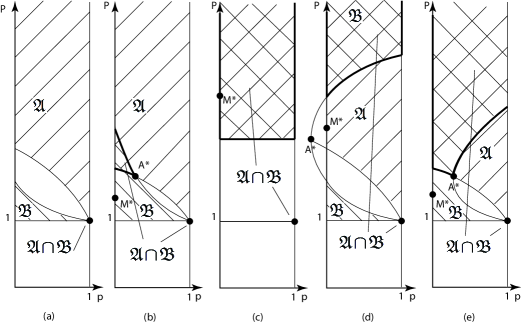
Figure 1 represents the position of the domains defined by the first ($\mathfrak{A}$) and the second ($\mathfrak{B}$) inequality in the cases (a) $\alpha_{+}=0,\ \alpha_{-}\in(0,1/2)$; (b) $\alpha_{+}=0,\ \alpha_{-}\geq 1/2$; (c) $\alpha_{+}>0,\ \alpha_{-}=0$; (d) $\alpha_{\pm}>0,\ \alpha_{+}+\alpha_{-}<1/2$; (e) $\alpha_{\pm}>0,\ \alpha_{+}+\alpha_{-}\geq 1/2$, respectively. The points $(1,1)$ and

$$A^{*}=\left(2-\frac{1}{\alpha_{-}+\alpha_{+}},\frac{1}{\alpha_{-}+\alpha_{+}}\right)$$

belong to the intersection of the boundaries of $\mathfrak{A},\ \mathfrak{B}$: $(1,1)$, $A^{*}\in\partial\mathfrak{A}\cap\partial\mathfrak{B}$.

In the case (a), it is clear that the unique point satisfying both inequalities is $p=P=1$, which implies the convergence of each profile at $+\infty$. In the cases (b)-(e), however, the final result depends strongly on the position of $M^{*}$. If $M^{*}$ is situated as in the picture (d) (that is analytically expressed by (10)) or as in pictures (b) and (e) (that is, $M^{*}<1/(\alpha_{+}+\alpha_{-})$), then the upper part of the intersection $\mathfrak{A}\cap\mathfrak{B}$ can be ignored so that $p=P=1$ and we obtain the convergence of all semi-wavefronts at $+\infty$. \qed

However, if the position of $M^{*}$ is as in the picture (c), there is a possibility of the co-existence of a monotone wavefront (recall here that $\alpha_{-}=0$ assures its existence in virtue of Fang and Zhao criterion) and a proper oscillating semi-wavefront. The main result of this paper consists precisely of the analytical proof of such a dynamical behaviour for certain systems with $\alpha_{-}=0$.

Remark 1

Clearly, the statement of Theorem 2 remains true if we replace $M^{*}$ with the smaller value $P=\limsup_{t\to+\infty}\phi(t)$. In the case (b), the condition $P<1/(\alpha_{+}+\alpha_{-})$ can be replaced by the dual inequality $p>2-1/(\alpha_{+}+\alpha_{-})$, where $p=\liminf_{t\to+\infty}\phi(t)$.

1.3 Case $\alpha_{-}=0$: the co-existence of monotone traveling fronts and proper semi-wavefronts in the KPP-Fisher equation with advanced argument.

The recent work by Nadin et al. [32] has provided another argument supporting the conjecture about the co-existence of different dynamical patterns in equation (1). The authors of [32] have proposed the following substitute, with $K(s)=\delta(s+h)$, (called ”a toy model”) of (2):

$\displaystyle\phi^{\prime\prime}(t)-c\phi^{\prime}(t)=-\left\{\begin{array}[]{cc}A\phi(t),&\phi(t)\in[0,\theta),\\ 1-\phi(t+h),&\phi(t)\geq\theta,\end{array}\right.$ (13)

(actually, this equation is obtained from the original toy model from [32] by reversing time). The positive parameters $A,h$ and $\theta\in(0,1)$ satisfy the inequality $A\geq(1-\theta)/\theta$, which is the reminiscence of the sub-tangency condition at 00 of the classical KPP-Fisher nonlinearity. The piece-wise linear model (13) inherits the local properties at the steady states from (1) and therefore it can be used to understand the geometry of the semi-wavefronts to (1). It is a remarkable fact that the computations of [32] predicted the co-existence of asymptotically periodic semi-wavefronts and monotone as well as oscillating wavefronts in equation (1). Nevertheless, the toy model (13) has one important deficiency: the right hand side of (13) is a discontinuous functional. At a first glance, precisely this drawback could be considered as a main reason for the existence of multiple semi-wavefronts. Indeed, let us consider the following ”delayed” toy model:

$\displaystyle\phi^{\prime\prime}(t)-c\phi^{\prime}(t)=-\left\{\begin{array}[]{cc}\phi(t),&\phi(t)\in[0,0.5),\\ 1-\phi(t-c\tau),&\phi(t)\geq 0.5,\end{array}\right.$ (16)

where $c=2.5$, $c\tau=2\ln 1.5=0.8109\dots$ (so that $\tau=0.8\ln 1.5=0.3243\dots<1/e=0.3678\dots$). It is easy to check that the eigenvalues of (16) at 00 are $0.5$ and $2$, while the set of all eigenvalues at $1$ contains two negative numbers $-0.5$ and $-4.035\dots$ This information allows us to construct two different monotone wavefronts $\phi_{j}\in W^{2,\infty}({\mathbb{R}})$ to (16):

$\displaystyle\phi_{1}(t)=\left\{\begin{array}[]{cc}0.5e^{0.5t},&\\ 1-0.5e^{-0.5t},&\end{array}\right.\phi_{2}(t)=\left\{\begin{array}[]{cc}0.5e^{2t},&t\leq 0,\\ 1-0.28..e^{-0.5t}-0.21..e^{-4.03..t},&t>0.\end{array}\right.$

Even more surprisingly, an oscillating wavefront to (16) can also be constructed. Indeed, since $x_{0}\pm iy_{0},\ x_{0}=-6.2402\dots,\ y_{0}=10.054\dots$ is a pair of conjugated eigenvalues to the equation (16) at the steady state $1$, it is easy to find the following oscillating profile $\phi_{3}\in W^{2,\infty}({\mathbb{R}})$:

$\displaystyle\phi_{3}(t)=\left\{\begin{array}[]{cc}0.5e^{2t},&t\leq 0,\\ 1+\hat{a}e^{x_{0}t}\cos(y_{0}t+z_{0}),&t>0,\end{array}\right.$

where

$$\hat{a}=\frac{1}{4}+\frac{(1-0.5x_{0})^{2}}{y_{0}^{2}}=0.546\dots,\quad\cos(z_{0})=-\frac{0.5}{\hat{a}},\ z_{0}=2.727\dots$$

See Figure 2 where all three solutions are shown.

Refer to caption
Figure 2: Co-existence of monotone and oscillating wavefronts in a delayed toy model.

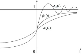
However, in view of the results mentioned in Subsection 1.1, this equation should possess a unique wavefront (up to a translation). Moreover, the wavefront $\phi_{2}$ decreases rapidly at $-\infty$ (i.e. $\phi_{2}$ is a pushed front) that is formally not compatible with the above mentioned sub-tangency condition $A\geq(1-\theta)/\theta$. It is clear that the discontinuity of equation (16) is the main reason of all these ”contradictions”.

Hence the conclusions suggested by the analysis of the ”toy” models must be corroborated by rigorous analytical proofs. In the present work, using Hale–Lin method [20] adapted for the singular functional differential equations in [11, 14, 16]; Hale–Huang analysis of the perturbed periodic solutions developed in [8, 18, 19, 23]; Krisztin–Walther–Wu theory of an invariant stratification of an attracting set for delayed monotone positive feedback [25]; Magalhães–Faria normal forms for retarded functional-differential equations [12] and Mallet-Paret–Sell theory of monotone cyclic feedback systems with delay [29, 30], we provide such a result:

Theorem 3

For each $\tau>3\pi/2$ sufficiently close to $3\pi/2$ there exists $c_{*}(\tau)>2$ and an open subset $\Omega$  of  ${\mathbb{R}}^{3}$ such that the KPP-Fisher equation with advanced argument

$$u_{t}(t,x)=u_{xx}(t,x)+u(t,x)(1-u(t+\tau,x)),\ u\geq 0,\ x\in{\mathbb{R}},$$

has a three-dimensional family $u(t,x)=\phi(x+ct,\zeta,c),\ \zeta\in\Omega,$ of wavefronts for each $c>c_{*}(\tau)$. For every fixed $c$, this family contains a unique (up to a translation) monotone wavefront and maps continuously and injectively $\Omega$ into the space $C_{b}({\mathbb{R}},{\mathbb{R}})$ of bounded continuous functions on ${\mathbb{R}}$. Moreover, for each $c>c_{*}(\tau)$, the above equation possesses proper semi-wavefronts $u(t,x)=\psi(x+ct,c)$. The profiles $\psi(\cdot,c)$ are asymptotically periodic at $+\infty$, with $\omega(c)$-periodic limit functions $\psi_{\infty}(\cdot,c)$ having periods $\omega(c)$ close to $2\pi c$ and of the sinusoidal form (i.e. each $\psi_{\infty}(\cdot,c)$ oscillates around 1 and has exactly two critical points on the period interval $[0,\omega(c))$).

Theorem 3 shows that the non-local KPP-Fisher equations with $\alpha_{+}\gg\alpha_{-}$ may exhibit multiple patterns of wave propagation:

Corollary 1

There exists $c>2$ and an increasing function $m:{\mathbb{R}}\to{\mathbb{R}}$ satisfying $m(-\infty)=0,$ $m(+\infty)=1$ such that equation (7) has, at the same time, a unique monotone wavefront, multiple oscillating wavefronts as well as asymptotically periodic proper semi-wavefronts propagating with the velocity $c$.

The structure of this paper is as follows. In Section 2 we establish a series of auxiliary results and a priori estimates necessary to prove Theorems 1 and 2. Section 3 contains the proof of Theorem 1. The first part of Theorem 3 (stated as Theorem 5) is proved in Sections 4, 5. The second part of Theorem 3 (stated as Theorem 7) is proved in Section 6 of our work.

2 A priori estimates and the convergence of semi-wavefronts

As it was suggested in [21], it is convenient to study equation (2) together with

$\displaystyle\phi^{\prime\prime}(t)-c\phi^{\prime}(t)+g_{\beta}(\phi(t))(1-(\phi*K)(t))=0,$ (19)

where the continuous piece-wise linear function $g_{\beta},\ \beta>1,$ is given by

$\displaystyle g_{\beta}(u)=\left\{\begin{array}[]{cc}u,&u\in[0,\beta],\\ \max\{0,2\beta-u\},&u>\beta.\end{array}\right.$ (22)

Observe that equation (19) has three constant solutions: $\phi(t)\equiv 0,1,2\beta$. We have the following

Lemma 1

Assume that $\phi,\ \phi(-\infty)=0,$ is a non-negative, bounded and non-constant solution of (19). Then $\phi(t)\leq 2\beta$ for all $t\in{\mathbb{R}}$. Next, if either $t_{0}$ is a point of local maximum for $\phi(t)$ with $\phi(t_{0})<2\beta$ or $t_{0}$ is the smallest number such that $\phi(t_{0})=2\beta$, then $(\phi*K)(t_{0})\leq 1$.

Proof 1

On the contrary, suppose that there exists a maximal interval $(t_{0},t_{1})$, such that $\phi(t)>2\beta=\phi(t_{0})$ for all $t\in(t_{0},t_{1})$. Then $\phi^{\prime}(t_{*})>0,\phi(t_{*})>2\beta$ for some $t_{*}\in(t_{0},t_{1})$. It follows from (19) and the definition of $g_{\beta}$ that $\phi^{\prime\prime}(t)=c\phi^{\prime}(t)$ for all $\ t\in(t_{0},t_{1})$. Hence, $\phi^{\prime}(t)=\phi^{\prime}(t_{*})e^{c(t-t_{*})}>0,$ $t\in(t_{0},t_{1})$ and therefore $t_{1}=+\infty$, $\phi(+\infty)=+\infty$, contradicting the boundedness of $\phi$.

Finally, if $t_{0}$ is a point of local maximum for $\phi(t)$, then $\phi^{\prime}(t_{0})=0,$ $\phi^{\prime\prime}(t_{0})\leq 0$. If, in addition, $\phi(t_{0})<2\beta$ then $g_{\beta}(\phi(t_{0}))>0$ and thus (19) assures that $(\phi*K)(t_{0})\leq 1$. In the case when $t_{0}$ is the smallest number such that $\phi(t_{0})=2\beta$, then clearly there exists a sequence $t_{j}\to t_{0},$ $t_{j}<t_{0},\ j=1,2,\dots$ such that $\phi^{\prime}(t_{j})>0,\ \phi^{\prime\prime}(t_{j})<0,\ \phi(t_{j})<2\beta$. But then $(\phi*K)(t_{j})<1,$ for all $j$ and therefore also $(\phi*K)(t_{0})\leq 1$. \qed

The following property of solutions to (2) and (19) was established in [4, Lemmas 3.7 and 3.9]:

Lemma 2

Assume that $\phi$ is a non-negative, bounded and non-constant solution of (19) or (2). If, in addition, $\phi(t_{n})\to 0$ along some sequence $t_{n}\to-\infty,$ then $\phi(t)$ is increasing on some interval $(-\infty,\rho],\ \phi(-\infty)=0,$ and  $\liminf_{t\to+\infty}\phi(t)>0.$

In fact, it is easy to see that each non-trivial non-negative profile should be positive:

Lemma 3

Let a non-negative bounded $\phi\not\equiv 0$ solve either (19) or (2) and $c\geq 2$. Then

$$\phi(t)>0,\quad-\phi^{\prime}(t)/\phi(t)>-\lambda(c).$$

If, in addition, $\phi(-\infty)=0,$ $\phi(t)\leq 1,\ t\in{\mathbb{R}},$ then $\phi^{\prime}(t)>0$ for all $t\in{\mathbb{R}}$ and $\phi(+\infty)=1$.

Proof 2

First, notice that equation (19) with $\beta=+\infty$ coincides with (2), so it suffices to consider equation (19) allowing $\beta=+\infty$. Suppose that, for some $s$, solution $\phi$ of (19) satisfies $\phi(s)=0$. Since $\phi(t)\geq 0,\ t\in{\mathbb{R}},$ this yields $\phi^{\prime}(s)=0$. Notice that $y=\phi(t)$ is the solution of the following initial value problem for a linear second order ordinary differential equation

$$y^{\prime\prime}(t)-cy^{\prime}(t)+a(t)y(t)=0,\quad y(s)=y^{\prime}(s)=0,$$

where

$$a(t):=\left\{\begin{array}[]{cc}1-(\phi*K)(t),&0\leq\phi(t)\leq\beta,\\ \frac{g_{\beta}(\phi(t))}{\phi(t)}(1-(\phi*K)(t)),&\phi(t)>\beta,\end{array}\right.$$

is a continuous bounded function. But then $y(t)\equiv 0$ due to the uniqueness theorem, a contradiction.

Suppose now that $\phi$ satisfies (19) and $c>2$. Set

$${\mathcal{N}}(\phi)(t):=g_{\beta}(\phi(t))(\phi*K)(t)+\phi(t)-g_{\beta}(\phi(t)),$$

then ${\mathcal{N}}(\phi)(t)>0$ and

$$\phi(t)=\frac{1}{\mu-\lambda}\int_{t}^{+\infty}(e^{\lambda(t-s)}-e^{\mu(t-s)}){\mathcal{N}}(\phi)(s)ds.$$ (23)

As a consequence, we have that

$$\phi^{\prime}(t)=\frac{1}{\mu-\lambda}\int_{t}^{+\infty}(\lambda e^{\lambda(t-s)}-\mu e^{\mu(t-s)}){\mathcal{N}}(\phi)(s)ds,$$

and therefore

$$\phi^{\prime}(t)-\lambda\phi(t)=-\int_{t}^{+\infty}e^{\mu(t-s)}{\mathcal{N}}(\phi)(s)ds<0.$$

If now $c=2$, we find similarly that

$$\phi(t)=\int_{t}^{+\infty}(s-t)e^{t-s}{\mathcal{N}}(\phi)(s)ds,\quad\phi^{\prime}(t)=\int_{t}^{+\infty}(s-t-1)e^{t-s}{\mathcal{N}}(\phi)(s)ds,$$

and thus also

$$\phi^{\prime}(t)-\phi(t)=-\int_{t}^{+\infty}e^{t-s}{\mathcal{N}}(\phi)(s)ds<0.$$

Finally, $0<\phi(t)\leq 1,\ t\in{\mathbb{R}},$ implies that $\phi^{\prime\prime}(t)-c\phi^{\prime}(t)\leq 0$. As a consequence, $\phi^{\prime}(s)\geq\phi^{\prime}(t)e^{c(s-t)},\ s\leq t$, so that there either exists a sequence $t_{n}\to+\infty$ such that $\phi^{\prime}(t_{n})>0$, or there exists the leftmost $T_{1}\in{\mathbb{R}}\cup\{+\infty\}$ such that $\phi^{\prime}(t)\leq 0$ for all $t\geq T_{1}$. In the first case, $\phi^{\prime}(t)>0,\ t\in{\mathbb{R}},$ while in the second case $\phi(t)$ is non-increasing and $\phi^{\prime\prime}(t)\leq c\phi^{\prime}(t)\leq 0,$ for $\ t\geq T_{1}$. Since $\phi(t)>0$, this can only happen when $\phi(t)\equiv\phi(T_{1})$ for $\ t\geq T_{1}$. But then $(\phi*K)(T_{1})=1$, which implies $\phi(t)=1$ for $t\geq T_{1}$ and $K(s)=0$ a.e. on ${\mathbb{R}}_{+}$. Furthermore, $\phi^{\prime}(s)>0$ for $s<T_{1}$. Now, observe that both $\phi(t)$ and $1$ satisfy equation (23) and that ${\mathcal{N}}(\phi)(t)={\mathcal{N}}(1)(t)=1$ for all $t\geq T_{1}$ and ${\mathcal{N}}(\phi)(t)=\phi(t)(\phi*K)(t)$ for $t\leq T_{1}$. Therefore (23) implies that, for $t<T_{1}$ close to $T_{1}$,

$$0<1-\phi(t)=\frac{1}{\mu-\lambda}\int_{t}^{T_{1}}(e^{\lambda(t-s)}-e^{\mu(t-s)})(1-\phi(s)(\phi*K)(s))ds\leq$$
$$\frac{1}{\mu-\lambda}\int_{t}^{T_{1}}(e^{\lambda(t-s)}-e^{\mu(t-s)})ds(1-\phi^{2}(t))=(t-T_{1})^{2}(0.5+o(1))(1-\phi(t))(1+\phi(t)),\ t\to T_{1}-,$$

a contradiction. \qed

Lemma 4

Let a positive bounded $\phi$ solve (19) and there exists the limit $\phi(+\infty)$. Then $\phi(+\infty)\in\{1,2\beta\}.$ If $\phi(+\infty)=2\beta$ then $\phi(t)\equiv 2\beta$ on some maximal nonempty interval $[T_{1},+\infty)$ and $(\phi*K)(T_{1})\leq 1$. Furthermore, if ${2}\beta\int_{-\infty}^{0}K(s)ds>1$ then $\phi(+\infty)=1$.

Proof 3

It follows from Lemmas 1 and 2 that $\phi(+\infty)\in(0,2\beta]$. In addition, if $\phi(+\infty)\not\in\{{1},2\beta\},$ then for

$$r(t):=g_{\beta}(\phi(t))(1-(\phi*K)(t)),$$

we have that

$$\lim_{t\to+\infty}r(t)=g_{\beta}(\phi(+\infty))(1-\phi(+\infty))\not=0.$$

However, in this case the differential equation $\phi^{\prime\prime}(t)-c\phi^{\prime}(t)+r(t)=0$ does not have any convergent solution on ${\mathbb{R}}_{+}$. Indeed, we have that

$$|\phi^{\prime}(t)|=\left|\phi^{\prime}(s)+c(\phi(t)-\phi(s))-\int_{s}^{t}r(u)du\right|\to+\infty\ \mbox{as}\ t\to+\infty.$$

Finally, assume that $\phi(+\infty)=2\beta$, then there exists $T_{1}\in{\mathbb{R}}$ such that $r(t)\leq 0$ for $t\in[T_{1},\infty)$ and thus $\phi^{\prime\prime}(t)-c\phi^{\prime}(t)\geq 0$ for $t\geq T_{1}$. As a consequence, $\phi^{\prime}(t)\geq\phi^{\prime}(s)e^{c(t-s)}$ for $t\geq s\geq T_{1}$. If $\phi^{\prime}(s)>0$ for some $s\geq T_{1}$, we obtain a contradiction: $\phi^{\prime}(+\infty)=+\infty$. Therefore we have to analyse the case when $\phi^{\prime}(s)=0$ for all $s\geq T_{1}$ (we can assume that $T_{1}$ is the smallest number with such a property). By Lemma 1,

$${2}\beta\int_{-\infty}^{0}K(s)ds=\int_{-\infty}^{0}\phi(T_{1}-s)K(s)ds\leq(\phi*K)(T_{1})\leq 1,$$

which proves the last statements of the lemma. \qed

Remark 2

Suppose that $\int_{-\infty}^{0}K(s)ds>0$. Then we can choose $\beta$ large enough to meet the inequality ${2}\beta\int_{-\infty}^{0}K(s)ds>1$. Hence, if $\int_{-\infty}^{0}K(s)ds>0$ and there exists $\phi(+\infty)$, we can assume that $\phi(+\infty)=1$.

Now, the change of variables

$$\phi(t)=e^{-x(t)},\;\;i.e.\;\;x(t)=-\ln\phi(t),$$ (24)

transforms equation (2) into

$$x^{\prime\prime}(t)-cx^{\prime}(t)-(x^{\prime}(t))^{2}+\left(\int_{-\infty}^{+\infty}e^{-x(t-s)}K(s)ds-1\right)=0,\ t\in{\mathbb{R}}.$$

We will also consider the family of equations

$$x^{\prime\prime}(t)-cx^{\prime}(t)-(x^{\prime}(t))^{2}+h_{\beta}(x(t))\left(\int_{-\infty}^{+\infty}e^{-x(s)}K(t-s)ds-1\right)=0,\ t\in{\mathbb{R}},$$

where non-decreasing continuous function $h_{\beta}:{\mathbb{R}}\to[0,+\infty)$ $\beta>1,$ is defined by

$$h_{\beta}(x)=\left\{\begin{array}[]{cc}1,&x\geq-\ln\beta,\\ \max\{0,2\beta e^{x}-1\},&x\leq-\ln\beta.\end{array}\right.$$

For $c\geq 2$, we will consider a strictly increasing function $f:[-1,\infty)\to{\mathbb{R}}$,

$$f(s):=\frac{2s}{c+\sqrt{c^{2}+4s}}.$$
Lemma 5

For each $c\geq 2$ and $K\in\mathcal{K}:=\{K\in L^{1}({\mathbb{R}},{\mathbb{R}}_{+}):|K|_{1}=1,K\geq 0\}$ there exists $U(c,K)\geq 1$ depending only on $c$ and $K$ such that the following holds: if $\phi(t)$, $\phi(-\infty)=0$, is a positive bounded solution of equation (19) with $\beta>U(c,K)$, then

$$0<\phi(t)\leq U(c,K),\ t\in{\mathbb{R}}$$ (25)

(i.e. the set of all semi-wavefronts to (19) is uniformly bounded by a constant which does not depend on a particular semi-wavefront). Moreover, given a fixed pair $(c_{0},K_{0})\in[2,+\infty)\times\mathcal{K}$, we can assume that the map $U:[2,+\infty)\times\mathcal{K}\to(0,+\infty)$ is locally continuous at $(c_{0},K_{0})$.

Proof 4

First, we take $U(c,K)\geq 1$ defined by one of the following non-exclusive formulas:

  • 1.

    if $\int_{0}^{+\infty}K(s)ds>0$, then $U(c,K)=\left(\int_{0}^{+\infty}e^{sf(-1)}K(s)ds\right)^{-1}$;

  • 2.

    if $\int_{0}^{+\infty}K(s)ds<0.001$, then $U(c,K)=2\exp{(\lambda(r+\sigma))},$ where $\lambda=\lambda(c)$ is defined by (6) and $r=r(K)\in{\mathbb{N}},\ \sigma=\sigma(c)>0$ are chosen in such a way that

    $$\int^{0}_{-r}K(s)ds>0.99,\quad 2c\frac{e^{\lambda\sigma}-1}{e^{c\sigma}-1}<0.01.$$

Obviously, such $U:[2,+\infty)\times\mathcal{K}\to(0,+\infty)$ is locally continuous at each $(c_{0},K_{0})$. For example, $U(c,K)$ can be considered as a constant (hence, continuous) function in some small neighborhood of $(c_{0},K_{0})\in[2,+\infty)\times\mathcal{K}$ satisfying $\int_{0}^{+\infty}K_{0}(s)ds=0$.

Clearly, if $\phi(t)\in(0,1]$ for all $t\in{\mathbb{R}}$, then inequality (25) is true because of $U(c,K)\geq 1$. In particular, this happens if the profile $\phi(t)$ is nondecreasing and $2\beta\int_{-\infty}^{0}K(s)ds>1$, see Remark 2.

Thus let us suppose that $\phi(t_{0})>1$ at some point $t_{0}$. Then at least one of the following three possibilities can occur:

Situation I. Solution $\phi(t)$ is nondecreasing and $\int_{-\infty}^{0}K(s)ds=0$ (so that $\int_{0}^{+\infty}K(s)ds=1$). In such a case, by Lemma 4, there is some finite $T_{1}$ such that $\phi(+\infty)=\phi(T_{1})=2\beta$ and $(\phi*K)(T_{1})\leq 1$. For $x$ defined by (24), we have $x^{\prime}(t)=-\phi^{\prime}(t)/\phi(t)\geq-\lambda(c)=f(-1)$ for all $t\in{\mathbb{R}}$ and

$$\int_{0}^{+\infty}e^{-x(T_{1}-s)}K(s)ds\leq(\phi*K)(T_{1})=\int_{{\mathbb{R}}}e^{-x(T_{1}-s)}K(s)ds\leq 1.$$

Now, set $m:=\min_{s\in{\mathbb{R}}}x(s)$ and observe that $x(t)=x(T_{1})-\int^{T_{1}}_{t}x^{\prime}(s)ds\leq m+f(-1)(t-T_{1})$ for $t\leq T_{1}$. Thus

$$\int_{0}^{+\infty}e^{-m+sf(-1)}K(s)ds\leq\int_{0}^{+\infty}e^{{-}x(T_{1}-s)}K(s)ds\leq 1$$

and therefore

$$\frac{1}{2\beta}=\frac{1}{\phi(T_{1})}=e^{m}\geq\int_{0}^{+\infty}e^{sf(-1)}K(s)ds.$$

Thus we can take

$$2\beta=\phi(T_{1})\leq\left(\int_{0}^{+\infty}e^{sf(-1)}K(s)ds\right)^{-1}=U(c,K).$$

The latter shows that Situation I cannot occur if $2\beta>U(c,K)$.

Situation II. Solution $\phi(t)$ is not nondecreasing and $\int_{0}^{+\infty}K(s)ds>0.$ Then we can repeat the above arguments to conclude that, for the local maxima $\phi(t_{j})>1$ of $\phi$ we have that

$$\sup_{t\in{\mathbb{R}}}\phi(t)=\sup_{j}\phi(t_{j})\leq\left(\int_{0}^{+\infty}e^{sf(-1)}K(s)ds\right)^{-1}=U(c,K).$$

Situation III. Solution $\phi(t)$ is not nondecreasing and $\int_{0}^{+\infty}K(s)ds=0$. Suppose, on the contrary, that $\phi(t_{0})>U(c,K)=2\exp{(\lambda(r+\sigma))}$ for some $t_{0}$. Then $\phi(t)\geq 2$ on some maximal closed interval $[a,b]\ni t_{0}$. We claim that $b-a\geq r+\sigma$. Indeed, otherwise, since $\phi^{\prime}(t)\leq\lambda\phi(t),$ $\phi(a)=2,$ $\phi^{\prime}(a)\geq 0,$ $t_{0}-a<b-a,$ we get the following contradiction

$$\phi(t_{0})\leq\phi(a)\exp(\lambda(t_{0}-a))<2\exp(\lambda(b-a))\leq 2\exp(\lambda(r+\sigma)).$$

In consequence,

$$(\phi*K)(t)\geq\int_{-r}^{0}\phi(t-s)K(s)ds\geq 1.98,\quad t\in[a,a+\sigma],$$

so that $(1-(\phi*K)(t))\leq-0.98,\ t\in[a,a+\sigma],$ and $\phi^{\prime\prime}(t)-c\phi^{\prime}(t)>0,$ $\ t\in[a,a+\sigma]$. In particular, $\phi^{\prime}(t)>e^{c(t-a)}\phi^{\prime}(a)$ for all $a<t\leq a+\sigma$ and thus

$$2\exp(\lambda(t-a))\geq\phi(t)>2+\frac{1}{c}\{e^{c(t-a)}-1\}\phi^{\prime}(a),\quad a<t\leq a+\sigma.$$

Therefore

$$2e^{\lambda\sigma}>2+\frac{1}{c}\{e^{c\sigma}-1\}\phi^{\prime}(a),$$

so that $0\leq\phi^{\prime}(a)<0.01$. Next, let $[a_{-},b_{+}]\supseteq[a,b]$ be the maximal interval where $\phi(t)\geq 1.1$. Then, for all $t\in[a_{-},a+\sigma]$, we have $\phi^{\prime\prime}(t)-c\phi^{\prime}(t)>0$ since

$$(\phi*K)(t)\geq\int_{-r}^{0}\phi(t-s)K(s)ds\geq 0.99\cdot 1.1>1,\ t\in[a_{-},a+\sigma].$$

But then

$$\phi^{\prime}(t)<\phi^{\prime}(a)e^{c(t-a)}<0.01e^{c(t-a)},\ t\in[a_{-},a);$$
$$\phi(t)>2-\frac{0.01}{c}\{1-e^{c(t-a)}\}>2-\frac{0.01}{c}>1.9,\quad t\in[a_{-},a),$$

a contradiction (since $\phi(a_{-})=1.1$). \qed

Corollary 2

Assume that $c\geq 2$ and $K$ are fixed. Then, for each sufficiently large $\beta>1$, equations (19) and (2) share the same set of semi-wavefronts propagating at the velocity $c$.

Proof 5

Due to Lemma 5 and the definition of $g_{\beta}(u)$, it suffices to take $\beta>U(c,K)$. \qed

A stronger a priori estimate is based on the following assertion:

Lemma 6

Let $y$ be a bounded solution of the boundary problem

$$y^{\prime}(t)-cy(t)-y^{2}(t)+g(t)=0,\ y(b)=0,\ t\in(a,b],$$

where $c\geq 2$ and a continuous function $g$ satisfies

$$-1<A:=\inf_{s\in(a,b]}g(s).$$

Set $B:=\sup_{s\in(a,b]}g(s).$ If there exists $\omega:=\min_{s\in(a,b]}y(s)$ and $A<0$, then $\omega\geq{f(A)}.$ Similarly, if there exists $\gamma:=\max_{s\in(a,b]}y(s),$ then $\gamma\leq f(B).$

Proof 6

The above statements were proved in [21, Lemma 20] under additional condition $y(a)=0,$ but without assuming the existence of the global extrema of $y$ on $(a,b]$. It is easy to check that the latter condition (which is obviously weaker than $y(a)=0$) is sufficient to repeat all the arguments in the proof of [21, Lemma 20]. \qed

The next two results can be considered as improvements of Lemma 5.

Lemma 7

Let $c\geq 2$ and $\phi(t),\ \phi(-\infty)=0,$ be a bounded positive solution of equation (2). Set $\ \rho(u)=f(e^{-u}-1)$, $x(t)=-\ln\phi(t)$ and

$$m=\liminf_{t\to+\infty}x(t),\quad M=\limsup_{t\to+\infty}x(t).$$

Then

$$\int_{0}^{+\infty}e^{\rho(m)s}K(s)ds+\int_{-\infty}^{0}e^{\rho(M)s}K(s)ds\geq e^{M},$$
$$\int_{0}^{+\infty}e^{\rho(M)s}K(s)ds+\int_{-\infty}^{0}e^{\rho(m)s}K(s)ds\leq e^{m}.$$

Observe that the integrals in the statement of Lemma 7 (and in Lemma 8 below as well) can be infinite (i.e. equal to $+\infty$).

Proof 7

By Lemma 2, the wavefront profile $\phi(t)$ is increasing on some maximal interval $(-\infty,Q_{0})$ and $\liminf_{t\to+\infty}\phi(t)>0$. Moreover, if $\phi(t)$ is eventually monotone and $\beta$ is sufficiently large then $\phi(+\infty)=1$ by Lemmas 4 and 5. In such a case, $M=m=0$, which proves the lemma. Hence, we may assume that $\phi(t)$ is not eventually monotone. Set $y(t)=x^{\prime}(t)$, since $x(t)$ is neither eventually monotone there exists some $s>Q_{0}$ such that $y(s)>0$. Moreover, it is clear that for each such $s$ we can find some finite $a<s<b$ such that $y(s)>0=y(b)=y(a)$. Then Lemmas 6 and 5 assure that

$$y(s)\leq f\left(\max_{t\in[a,b]}\int_{\mathbb{R}}e^{-x(t-u)}K(u)du-1\right)\leq f(U(c,K)-1).$$

In particular, this means that $\sup_{s\in{\mathbb{R}}}y(s)$ is a finite number. We claim that

$$\limsup_{s\to+\infty}y(s)\leq\rho(m).$$ (26)

Indeed, let $s_{j}\to+\infty$ be such that $y(s_{j})\to\limsup_{s\to+\infty}y(s)$. Then for appropriately chosen sequences $a_{j}<s_{j}<b_{j}$, $a_{j}\to+\infty$, we have that

$$y(s_{j})\leq f\left(\max_{t\in[a_{j},b_{j}]}\int_{\mathbb{R}}e^{-x(t-u)}K(u)du-1\right).$$

Next, by Lemma 5, for every small $\epsilon>0$ there exists $T=T(\epsilon,c,K),\ T(0^{+},c,K)=+\infty,$ such that

$$\int_{-T}^{T}K(u)du>1-\epsilon,\ \int_{-\infty}^{-T}e^{-x(t-u)}K(u)du+\int^{+\infty}_{T}e^{-x(t-u)}K(u)du<\epsilon,\ t\in{\mathbb{R}}.$$ (27)

Consequently,

$$y(s_{j})\leq f(\max_{t\in[a_{j}-T,b_{j}+T]}e^{-x(t)}-1+\epsilon).$$

Taking into account that $\liminf_{j\to\infty}\min_{t\in[a_{j}-T,b_{j}+T]}x(t)\geq m$, we conclude that

$$\limsup_{s\to+\infty}y(s)\leq f(e^{-m}-1+\epsilon).$$

Letting $\epsilon\to 0^{+}$ in the last inequality, we obtain (26).

Next, Lemma 3 implies that $y(s)>f(-1)\geq-1>-c$ for all $s\in{\mathbb{R}}$. Since $x(t)$ is not eventually monotone, there exist sequences $d_{j}<\varsigma_{j}<e_{j}$, $d_{j}\to+\infty,$ such that $\min_{s\in[d_{j},e_{j}]}y(s)=y(\varsigma_{j})<0=y(d_{j})=y(e_{j})$ and $y(\varsigma_{j})\to\liminf_{s\to+\infty}y(s)$. Set $g(t)=\int_{\mathbb{R}}e^{-x(t-u)}K(u)du-1$. Since $y^{\prime}(\varsigma_{j})=0$, we obtain that

$$-1<\min_{s\in[d_{j},e_{j}]}g(s)\leq g(\varsigma_{j})=y^{2}(\varsigma_{j})+cy(\varsigma_{j})<0.$$

Therefore Lemma 6 can be applied yielding

$$y(\varsigma_{j})\geq f\left(\min_{t\in[d_{j},e_{j}]}\int_{\mathbb{R}}e^{-x(t-u)}K(u)du-1\right).$$

From this estimation, arguing as above, we deduce that

$$\liminf_{s\to+\infty}y(s)\geq\rho(M)>f(-1).$$

Next, let $t_{j}\to+\infty$ be a sequence of local maximum points of $x(t)$ such that $x(t_{j})\to M$ as $j\to+\infty$. With $T$ and $\epsilon$ as in (27) and for sufficiently large $j$, we find that

$$m^{\prime}_{j}:=\min_{s\in[t_{j},t_{j}+T]}x^{\prime}(s)>\rho(M)-\epsilon,\ M^{\prime}_{j}:=\max_{s\in[t_{j},t_{j}+T]}x^{\prime}(s)<\rho(m)+\epsilon,$$
$$m_{j}:=\min_{[t_{j}-T,t_{j}+T]}x(s)>m-\epsilon,\ M_{j}:=\max_{[t_{j}-T,t_{j}+T]}x(s)<M+\epsilon,$$
$$\epsilon+\int_{-T}^{T}e^{-x(t_{j}-s)}K(s)>\int_{{\mathbb{R}}}e^{-x(t_{j}-s)}K(s)ds\geq 1,$$
$$x(t)\geq x(t_{j})+m^{\prime}_{j}(t-t_{j})\geq x(t_{j})+(\rho(M)-\epsilon)(t-t_{j}),\ t\in[t_{j},t_{j}+T],$$
$$x(t)\geq x(t_{j})+M^{\prime}_{j}(t-t_{j})\geq x(t_{j})+(\rho(m)+\epsilon)(t-t_{j}),\ t\in[t_{j}-T,t_{j}].$$

Therefore, for each subset $[A,B]\subset[-T,T],\ A\leq 0\leq B,$ we obtain

$$\epsilon+\int_{-T}^{0}e^{-x(t_{j}-s)}K(s)ds+\int_{0}^{T}e^{-x(t_{j}-s)}K(s)ds>1,$$
$$\epsilon+\int^{A}_{-T}e^{-m+\epsilon}K(s)ds+\int_{A}^{0}e^{-x(t_{j})+(\rho(M)-\epsilon)s}K(s)ds+$$
$$\int_{0}^{B}e^{-x(t_{j})+(\rho(m)+\epsilon)s)}K(s)ds+\int_{B}^{T}e^{-m+\epsilon}K(s)ds>1.$$

Taking limit in the last inequality when $\epsilon\to 0$ (so that $T\to+\infty$), $j\to+\infty$, we obtain that

$\displaystyle e^{-m}\left(\int^{A}_{-\infty}K(s)ds+\int_{B}^{+\infty}K(s)ds\right)+e^{-M}\left(\int_{A}^{0}e^{\rho(M)s}K(s)ds+\int_{0}^{B}e^{\rho(m)s}K(s)ds\right)\geq 1.$ (28)

This relation is valid for each $-\infty\leq A\leq 0\leq B\leq+\infty$ and if $A,B$ are infinite, we get the first inequality of the lemma. Clearly, the second inequality can be deduced in a similar way from

$\displaystyle e^{-M}\left(\int^{A^{\prime}}_{-\infty}K(s)ds+\int_{B^{\prime}}^{+\infty}K(s)ds\right)+e^{-m}\left(\int_{A^{\prime}}^{0}e^{\rho(m)s}K(s)ds+\int_{0}^{B^{\prime}}e^{\rho(M)s}K(s)ds\right)\leq 1,$ (29)

where $A^{\prime},B^{\prime}$ are arbitrary real numbers satisfying $-\infty\leq A^{\prime}\leq 0\leq B^{\prime}\leq+\infty$. \qed

Lemma 8

Let $\phi(t)$ be a semi-wavefront to equation (2) propagating with the speed $c\geq 2$. Set

$$p=\liminf_{t\to+\infty}\phi(t),\ P=\limsup_{t\to+\infty}\phi(t),\ \alpha_{+}:=\frac{1}{c}\int_{-\infty}^{0}|s|K(s)ds,\ \alpha_{-}:=\frac{1}{c}\int^{+\infty}_{0}sK(s)ds.$$

Then $0<p\leq 1\leq P$ and

$$p+\alpha_{+}P(1-p)+\alpha_{-}P(P-1)\geq 1,$$ (30)
$$P-\alpha_{+}P(P-1)-\alpha_{-}P(1-p)\leq 1.$$ (31)
Proof 8

Taking $A=B=A^{\prime}=B^{\prime}=0$ in (28), (29) we find immediately that $0<p\leq 1\leq P$. In the case when $p=P$, Lemma 4 and Corollary 2 imply that $p=P=1$ and that proves the lemma. If $p<P$, $\phi(t)$ oscillates between $p$ and $P$. Therefore $\phi^{\prime}(t)$ is oscillating around 00 and there exist finite limits

$$d=\liminf_{t\to+\infty}\phi^{\prime}(t)\leq 0\leq D:=\limsup_{t\to+\infty}\phi^{\prime}(t).$$

We claim that

$$-\frac{1}{c}P(P-1)\leq d\leq D\leq\frac{1}{c}P(1-p).$$

Indeed, let $t_{j}\to+\infty$ be such that $0>\phi^{\prime}(t_{j})\to d,\ \phi^{\prime\prime}(t_{j})=0$. Then

$$-\phi^{\prime}(t_{j})=\frac{1}{c}\phi(t_{j})(\phi*K(t_{j})-1).$$

For an arbitrary $\epsilon>0$, we fix $T$ sufficiently large to have

$$\int_{-\infty}^{-T}\phi(t-s)K(s)ds+\int^{+\infty}_{T}\phi(t-s)K(s)ds<\epsilon,\quad t\in{\mathbb{R}}.$$

Then

$$-\phi^{\prime}(t_{j})\leq\frac{1}{c}\phi(t_{j})\left(\epsilon+\int_{-T}^{T}\phi(t_{j}-s)K(s)ds-1\right)$$
$$\leq\frac{1}{c}\sup_{u\geq 0.5t_{j}}\phi(u)\left(\epsilon+\sup_{u\geq 0.5t_{j}}\phi(u)\int_{-T}^{T}K(s)ds-1\right).$$

After taking limit as $j\to+\infty,\ \epsilon\to 0^{+}$ (so that $T\to+\infty$), we get one of the required relations: $-d\leq P(P-1)/c$. The second inequality can be proved similarly.

Next, consider the sequence $\{s_{j}\}$ of local maximum points such that $\phi(s_{j})\to P,$ $s_{j}\to+\infty$. We can suppose that $s_{j}$ is large enough to have

$$\min_{s\in[s_{j}-T,s_{j}+T]}\phi^{\prime}(s)\geq d-\epsilon,\quad\max_{s\in[s_{j}-T,s_{j}+T]}\phi^{\prime}(s)\leq D+\epsilon.$$

Then

$$\phi(s_{j}-s)\geq\phi(s_{j})-(D+\epsilon)s,\ \mbox{for}\ s\in[0,T],\quad\phi(s_{j}-s)\geq\phi(s_{j})-(d-\epsilon)s,\ \mbox{for}\ s\in[-T,0],$$

and therefore

$$1\geq\int_{-\infty}^{+\infty}\phi(s_{j}-s)K(s)ds\geq\int_{-T}^{T}\phi(s_{j}-s)K(s)ds\geq$$
$$\phi(s_{j})\int_{-T}^{T}K(s)ds-(D+\epsilon)\int_{0}^{T}sK(s)ds+(d-\epsilon)\int_{-T}^{0}|s|K(s)ds.$$

Finally, letting $\epsilon\to 0^{+}$ (hence, $T\to+\infty$), $s_{j}\to+\infty$, we get the required inequality

$$1\geq P-Dc\alpha_{-}+dc\alpha_{+}\geq P-\alpha_{-}P(1-p)-\alpha_{+}P(P-1).$$

The proof of inequality (30) is completely analogous and therefore it is omitted here. \qed

Remark 3

Inequality (31) has a simple geometric interpretation. Indeed, consider the following function

$$\tilde{\phi}_{-}(-s):=\left\{\begin{array}[]{cc}P-P(1-p)s/c,&s\geq 0,\\ P+P(P-1)s/c,&s\leq 0,\end{array}\right.$$

then inequality (31) can be written as $\tilde{\Theta}(p,P):=(K*\tilde{\phi}_{-})(0)\leq 1$. A serious drawback of the obtained estimate is that $\tilde{\Theta}(p,P)$ can be negative and therefore the relation $\tilde{\Theta}(p,P)\leq 1$ is not very useful. We can avoid this imperfection by introducing the function $\phi_{-}(-s,p,P):=\max\{p,\tilde{\phi}_{-}(-s)\}.$ Arguing as in the proof of Lemma 8, we can find that $p$ and $P$ should satisfy the following improved inequality $\Theta(p,P)=(K*\phi_{-})(0)\leq 1.$ Obviously, continuous function $\Theta(p,P)$ is non-negative for all $0\leq p\leq P$.

3 Existence of semi-wavefronts for $c\geq 2$.

In this section, we are going to prove Theorem 1. It should be observed that the necessity of the condition $c\geq 2$ can be easily obtained from the analysis of the asymptotic behaviour of eventual semi-wavefront $\phi$ at $-\infty$ (if $c<2$ then $\phi(t)$ oscillates around 00 at $-\infty$). Thus we have to prove only the sufficiency of the condition $c\geq 2$ for the existence of semi-wavefronts.

First, consider

$$r(\phi)(t):=b\phi(t)+g_{\beta}(\phi(t))(1-(\phi*K)(t)),$$

where $g_{\beta}(u)$ is defined by (22), $\beta$ is as in Corollary 2, and $b>1+2\beta$. In view of Corollary 2, it suffices to establish that the equation

$$\phi^{\prime\prime}(t)-c\phi^{\prime}(t)-b\phi(t)+r(\phi)(t)=0$$ (32)

has a semi-wavefront. Observe that if a continuous function $\psi(t),\ 0\leq\psi(t)\leq 2\beta,$ satisfies $0\leq\psi(s)\leq\beta$ at some point $s\in{\mathbb{R}}$, then

$$r(\psi)(s)=\psi(s)(b+1-(\psi*K)(s))\geq 0.$$ (33)

Now, if $\beta\leq\psi(s)\leq 2\beta$, then

$$r(\psi)(s)=b\psi(s)+(2\beta-\psi(s))(1-(\psi*K)(s))=$$
$$2\beta(1-(\psi*K)(s))+\psi(s)(b-1+(\psi*K)(s))>\beta.$$ (34)

Next, we consider the non-delayed KPP-Fisher equation $u_{t}=u_{xx}+g_{\beta}(u)$. The profiles $\phi$ of the traveling fronts $u(x,t)=\phi(x+ct)$ for this equation satisfy

$$\phi^{\prime\prime}(t)-c\phi^{\prime}(t)+g_{\beta}(\phi(t))=0,\ c\geq 2.$$ (35)

Recall that $0<\lambda\leq\mu$ denote eigenvalues of equation (35) linearized around 00 (i.e. $\chi(\lambda)=\chi(\mu)=0$ where $\chi(z):=z^{2}-cz+1$). In the sequel, $\phi_{+}(t)$ will denote the unique monotone front to (35) normalised (cf. [15, Theorem 6]) by the condition

$$\phi_{+}(t):=(-t)^{j}e^{\lambda t}(1+o(1)),\ t\to-\infty,\ j\in\{0,1\}.$$

Let us note here that $\phi_{+}(t)$ for all $t$ such that $\phi_{+}(t)<\beta,$ satisfies the linear differential equation

$$\phi^{\prime\prime}(t)-c\phi^{\prime}(t)+\phi(t)=0.$$

In particular, if $c>2$ then there exists (see e.g. [15, Theorem 6]) $C\geq 0$ such that

$$\phi_{+}(t):=e^{\lambda t}-Ce^{\mu t},\ t\leq\phi_{+}^{-1}(\beta).$$ (36)

Let $z_{1}<0<z_{2}$ be the roots of the equation $z^{2}-cz-b=0$. Set $z_{12}=z_{2}-z_{1}>0$ and consider the integral operator $A_{m}$ depending on $b$ and defined by

$$(A_{m}\phi)(t)=\frac{1}{z_{12}}\left\{\int_{-\infty}^{t}e^{z_{1}(t-s)}r(\phi(s))ds+\int_{t}^{+\infty}e^{z_{2}(t-s)}r(\phi(s))ds\right\}.$$
Lemma 9

Assume that $b>1+2\beta$ and let $0\leq\phi(t)\leq\phi_{+}(t)$, then

$$0\leq(A_{m}\phi)(t)\leq\phi_{+}(t).$$
Proof 9

The lower estimate is obvious since $0\leq\phi(t)\leq\phi_{+}(t)\leq 2\beta$ and therefore $r(\phi(t))\geq 0$ in view of (33) and (34). Now, since $\phi(t)\leq\phi_{+}(t)$ and $bu+g_{\beta}(u)$ is an increasing function, we find that

$$r(\phi(s))\leq b\phi(t)+g_{\beta}(\phi(t))\leq b\phi_{+}(t)+g_{\beta}(\phi_{+}(t))=:R(\phi_{+}(t)).$$

Thus

$$(A_{m}\phi)(t)\leq\frac{1}{z_{12}}\left\{\int_{-\infty}^{t}e^{z_{1}(t-s)}R(\phi_{+}(s))ds+\int_{t}^{+\infty}e^{z_{2}(t-s)}R(\phi_{+}(s))ds\right\}=\phi_{+}(t),$$

and the lemma is proved. \qed

Lemma 9 says that $\phi_{+}(t)$ is an upper solution for (32), cf. [37]. Still, we need to find a lower solution. Here, assuming that $c>2$ and that $K$ has a compact support we will use the following well known ansatz (see e.g. [37])

$$\phi_{-}(t)=\max\{0,e^{\lambda t}(1-Me^{\epsilon t})\},$$

where $\epsilon\in(0,\lambda)$ and $M\gg 1$ is chosen in such a way that $-\chi(\lambda+\epsilon)>(L/M)\int_{-\infty}^{\infty}e^{-\epsilon s}K(s)ds$ (here $L:=\sup_{t\in{\mathbb{R}}}\phi_{+}(t)e^{-\epsilon t}$), $\lambda+\epsilon<\mu$, and

$$0<\phi_{-}(t)<\phi_{+}(t)<e^{\epsilon t}<1,\quad t<T_{c},\ \mbox{where}\ \phi_{-}(T_{c})=0.$$

The above inequality $\phi_{-}(t)<\phi_{+}(t)$ is possible due to representation (36). We note also that $(\phi_{+}*K)(t)\leq Le^{\epsilon t}\int_{\mathbb{R}}e^{-\epsilon s}K(s)ds$.

Lemma 10

Assume that $c>2$, $K$ has a compact support, $b>2\beta+2$. Then the inequality $\phi_{-}(t)\leq\phi(t)\leq\phi_{+}(t),\ t\in{\mathbb{R}},$ implies that

$$\phi_{-}(t)\leq(A_{m}\phi)(t)\leq\phi_{+}(t),\quad t\in{\mathbb{R}}.$$ (37)
Proof 10

Due to Lemma 9, it suffices to prove the first inequality in (37) for $t\leq T_{c}$. Since $0<\phi(t)<1<\beta,\ t\leq T_{c}$, we have, for $t\leq T_{c}$, that

$$(A_{m}\phi)(t)\geq\frac{1}{z_{12}}\left\{\int_{-\infty}^{t}e^{z_{1}(t-s)}r(\phi(s))ds+\int_{t}^{T_{c}}e^{z_{2}(t-s)}r(\phi(s))ds\right\}=$$
$$\frac{1}{z_{12}}\left\{\int_{-\infty}^{t}e^{z_{1}(t-s)}\phi(s)(b+1-(\phi*K)(s))ds+\int_{t}^{T_{c}}e^{z_{2}(t-s)}\phi(s)(b+1-(\phi*K)(s))ds\right\}\geq$$
$$\frac{1}{z_{12}}\left\{\int_{-\infty}^{t}e^{z_{1}(t-s)}\Gamma(s)ds+\int_{t}^{T_{c}}e^{z_{2}(t-s)}\Gamma(s)ds\right\}=$$
$$\frac{1}{z_{12}}\left\{\int_{-\infty}^{t}e^{z_{1}(t-s)}\Gamma(s)ds+\int_{t}^{+\infty}e^{z_{2}(t-s)}\Gamma(s)ds\right\}=:Q(t),$$

where $\Gamma(s):=\phi_{-}(s)(b+1-(\phi_{+}*K)(s))$.

In order to estimate $Q(t)$, we first find, for $t\leq T_{c}$, that

$$\phi_{-}^{\prime\prime}(t)-c\phi_{-}^{\prime}(t)-b\phi_{-}(t)+b\phi_{-}(t)+\phi_{-}(t)(1-(\phi_{+}*K)(t))=$$
$$-\chi(\lambda+\epsilon)Me^{(\lambda+\epsilon)t}-(\phi_{+}*K)(t)e^{\lambda t}(1-Me^{\epsilon t})\geq-\chi(\lambda+\epsilon)Me^{(\lambda+\epsilon)t}-e^{\epsilon t}e^{\lambda t}L{\int_{-\infty}^{\infty}e^{-\epsilon s}K(s)ds}=$$
$$Me^{(\lambda+\epsilon)t}\left(-\chi(\lambda+\epsilon)-{\frac{L}{M}\int_{-\infty}^{\infty}e^{-\epsilon s}K(s)ds}\right)>0.$$

But then, rewriting the latter differential inequality in the equivalent integral form (see e.g. [26] or [34, Lemma 18]) and using the fact that

$$\Delta\phi^{\prime}_{-}|_{T_{c}}:=\phi^{\prime}_{-}(T_{c}^{+})-\phi^{\prime}_{-}(T_{c}^{-})=-\phi^{\prime}_{-}(T_{c}^{-})>0,$$

we can conclude that $Q(t)\geq\phi_{-}(t),\ t\in{\mathbb{R}}$. Hence, $(A_{m}\phi)(t)\geq\phi_{-}(t),\ t\in{\mathbb{R}}$. \qed

Next, with each vector $\mathfrak{m}=(\mu_{1},\mu_{2})$ we will associate the following Banach spaces:

$$C_{\mathfrak{m}}=\{y\in C({\mathbb{R}},{\mathbb{R}}):|y|_{\mathfrak{m}}:=\sup_{s\leq 0}e^{-\mu_{2}s}|y(s)|+\sup_{s\geq 0}e^{-\mu_{1}s}|y(s)|<+\infty\},$$
$$C^{1}_{\mathfrak{m}}=\{y\in C_{\mathfrak{m}}:y^{\prime}\in C_{\mathfrak{m}},\ |y|_{1,\mathfrak{m}}:=|y|_{\mathfrak{m}}+|y^{\prime}|_{\mathfrak{m}}<+\infty\}.$$
Remark 4

Observe that $C_{\mathfrak{m}}=C^{0}(\mu_{2},\mu_{1})$, $C^{1}_{\mathfrak{m}}=C^{1}(\mu_{2},\mu_{1})$ in the notation of [20, p. 185].

It is clear that, in order to establish the existence of semi-wavefronts to equation (32), it suffices to prove that the equation $A_{m}\phi=\phi$ has at least one solution from the set

$$\mathfrak{K}=\{x\in C_{\mathfrak{m}}:\phi_{-}(t)\leq x(t)\leq\phi_{+}(t),\ t\in{\mathbb{R}}\},$$

where ${\mathfrak{m}}=(\rho,\lambda/2)$ for some fixed $\rho>0$. Observe that the convergence $x_{n}\to x$ in $\mathfrak{K}$ is equivalent to the uniform convergence on compact subsets of ${\mathbb{R}}$.

Lemma 11

Let $c>2$. Then $\mathfrak{K}$ is a closed, bounded, convex subset of $C_{\mathfrak{m}}$ and $A_{m}:\mathfrak{K}\to\mathfrak{K}$ is completely continuous.

Proof 11

By the previous lemma, $A_{m}(\mathfrak{K})\subset\mathfrak{K}$. It is also obvious that $\mathfrak{K}$ is a closed, bounded, convex subset of $C_{\mathfrak{m}}$. Since

$$|x(t)|+|(A_{m}x)^{\prime}(t)|\leq 2\beta(1+z_{12}),\ \mbox{for all}\ x\in\mathfrak{K},$$ (38)

due to the Ascoli-Arzel${\rm\grave{a}}$ theorem $A_{m}(\mathfrak{K})$ is relatively compact in $\mathfrak{K}$ . Next, by Lebesgue’s dominated convergence theorem, if $x_{j}\to x_{0}$ in $\mathfrak{K}$ then $(A_{m}x_{j})(t)\to(A_{m}x_{0})(t)$ at every $t\in{\mathbb{R}}$. The precompactness of $\{A_{m}x_{j}\}\subset\mathfrak{K}$ assures that, in fact, $A_{m}x_{j}\to A_{m}x_{0}$ in $\mathfrak{K}$. Hence, the map $A_{m}:\mathfrak{K}\to\mathfrak{K}$ is completely continuous. \qed

The final steps of the proof of Theorem 1 are contained in the following proposition.

Theorem 4

Assume that $c\geq 2$. Then the integral equation $A_{m}\phi=\phi$ has at least one positive bounded solution in $\mathfrak{K}$.

Proof 12

Assume first that $K$ has a compact support. If $c>2$ then, due to the previous lemma, we can apply Schauder’s fixed point theorem to $A_{m}:\mathfrak{K}\to\mathfrak{K}$ that guarantees the existence of a fixed point for $A_{m}$ in $\mathfrak{K}$, which is a semi-wavefront profile for equation (1). Let now $c=2$ and consider $c_{j}:=2+1/j$. Since $c_{j}>2$, we already know that for each $j$ there exists a semi-wavefront $\phi_{j}$ of equation (32): we can normalise it by the condition $\phi_{j}(0)=1/2=\max_{s\leq 0}\phi_{j}(s)$. It is clear from (38) that the set $\{\phi_{j},j\geq 0\}$ is precompact in the compact-open topology of $C_{b}({\mathbb{R}},{\mathbb{R}})$ and therefore we can also assume that $\phi_{j}\to\phi_{0}$ uniformly on compact subsets of ${\mathbb{R}}$, where $\phi_{0}(0)=1/2=\max_{s\leq 0}\phi_{0}(s)$. In addition, $R_{j}(s):=r(\phi_{j}(s))\to R_{0}(s):=r(\phi_{0}(s))$ for each fixed $s\in{\mathbb{R}}$. The sequence $\{R_{j}(t)\}$ is also uniformly bounded on ${\mathbb{R}}$. All this allows us to apply Lebesgue’s dominated convergence theorem in

$$(A_{m,j}\phi_{j})(t):=\frac{1}{\epsilon_{j}^{\prime}}\left\{\int_{-\infty}^{t}e^{z_{1,j}(t-s)}R_{j}(s)ds+\int_{t}^{+\infty}e^{z_{2,j}(t-s)}R_{j}(s)ds\right\}=\phi_{j}(t),$$

where $z_{1,j}<0<z_{2,j}$ satisfy $z^{2}-c_{j}z-b=0$. In this way we obtain that $A_{m}\phi_{0}=\phi_{0}$ with $c=2$ and therefore $\phi_{0}$ is a non-negative solution of equation (2) satisfying condition $\phi_{0}(0)=1/2=\max_{s\leq 0}\phi_{0}(s)$. Lemma 3 shows that actually $\phi_{0}(t)>0$ for all $t\in{\mathbb{R}}$. We claim, in addition, that $\inf_{s\leq 0}\phi_{0}(s)=0$ and therefore $\phi_{0}(-\infty)=0$ in view of Lemma 2. Indeed, otherwise there exists a positive $k_{0}$ such that $k_{0}\leq\phi_{0}(t)\leq 1/2$ for all $t\leq 0$. This implies immediately that $k_{0}/4\leq a(t):=\phi_{0}(t)(1-(\phi_{0}*K)(t))\leq 3/4$ for all sufficiently large negative $t$ (say, for $t\leq t_{0}$). But then

$$\phi_{0}^{\prime}(t)=\phi_{0}^{\prime}(t_{0})+c(\phi_{0}(t)-\phi_{0}(t_{0}))+\int^{t_{0}}_{t}a(u)du\to+\infty\ \mbox{as}\ t\to-\infty,$$

contradicting the positivity of $\phi_{0}(t)$. In consequence, $\phi_{0}$ is a semi-wavefront.

Finally, in order to prove the theorem for general kernels, we can use a similar argument by constructing a sequence of compactly supported kernels $K_{j}$ converging monotonically to $K$. Indeed, set $K_{j}(s)=K(s)+\left(\int_{-\infty}^{-j}K(s)ds+\int_{j}^{\infty}K(s)ds\right)/(2j)$ for $s\in[-j,j]$, and set $K_{j}(s)=0$ otherwise. As we already proved, for each fixed $c\geq 2$ and $K_{j}$ there exists a semi-wavefront $\phi_{j}$ propagating with the velocity $c$ and satisfying the condition $\phi_{j}(0)=1/2=\max_{s\leq 0}\phi_{j}(s)$. Due to Lemma 5, $0<\phi_{j}(t)\leq U(c,K_{j})$ for all $t\in{\mathbb{R}}$. By using the explicit form of $U(c,K_{j})$ given in Lemma 5, it is easy to show that the sequence $\{\phi_{j}(t)\}$ is uniformly bounded on ${\mathbb{R}}$. Thus the sequence $\{\phi^{\prime}_{j}(t)\}$ is uniformly bounded on ${\mathbb{R}}$ as well, so we can assume that $\phi_{j}\to\phi_{0}\in C_{b}({\mathbb{R}},{\mathbb{R}})$ uniformly on compact subsets of ${\mathbb{R}}$. But then $\phi_{0}(0)=1/2=\max_{s\leq 0}\phi_{0}(s)$ so that, as we have recently seen, $\phi_{0}(x+ct)$ must be a semi-wavefront for equation (1). \qed

4 Proof of the first part of Theorem 3

In Sections 4 and 5, we show that the non-local KPP-Fisher equation (1) can possess multiple wavefront solutions. It is convenient to split our proof into two stages. In the next section, we are doing all standard technical work related to the application of the Lyapunov-Schmidt reduction. This allows us to focus our attention in the present section on the new ideas of the proof.

We start by analysing zeros of the function $\chi_{1}(z):=z-\exp(-z\tau)$:

Lemma 12

The function $\chi_{1}(z)$ has exactly three simple zeros (denoted as $z_{1}(\tau)\in(0,1),$ $z_{2}(\tau)$ and $z_{3}(\tau)=\bar{z}_{2}(\tau)\in{\mathbb{C}}$) in the half-plane $\{\Re z\geq 0\}$ and does not have any root on the imaginary axis $\{\Re z=0\}$ if and only if $\tau\in(3\pi/2,7\pi/2).$ Furthermore, $\Re z_{2}(\tau)<z_{1}(\tau)$.

Proof 13

By applying the Rouché theorem in the domains $D_{R}\ni\{0\}$ bounded by the graphs of $\{\Re z=-2\}$ and $\{|z|=R\}$, $R>0$, we easily find that the half-plane $\{\Re z>-2\}$ contains only one zero $z_{1}$ of $\chi_{1}(z)$ for every $\tau\in[0,0.5\ln 2)$. It is clear that $z_{1}>0$ if $\tau>0$. Since $\tau>0$, all zeros of $\chi_{1}(z)$ are simple. This means that when $\tau$ is increasing from the initial value $0.5\ln 2$, each new pair of roots appearing in the half-plane $\{\Re z>0\}$ should cross the imaginary axis $\{\Re z=0\}$ at some moment $\tau_{n}$. It is easy to check that the first pair of complex conjugated roots $z_{2}(\tau),z_{3}(\tau)$ will cross transversally $\{\Re z=0\}$ at the point $\tau=3\pi/2$ with the velocity $\Re z_{j}^{\prime}(\tau)|_{\tau=3\pi/2}>0$. The same happens with each other pair of roots crossing $\{\Re z=0\}$ at the moments $\tau_{n}=3\pi/2+2\pi n$. Finally, $\Re z_{2}(\tau)<z_{1}(\tau)$ for all $\tau$ such that $\tau-3\pi/2$ is small and positive. If $\Re z_{2}(\tau_{0})=z_{1}(\tau_{0})$ then $|z_{2}|=|\exp(-z_{2}\tau)|=|\exp(-z_{1}\tau)|=z_{1}$ so that $\Im z_{2}=0$, a contradiction. \qed

Theorem 5

For each $\tau\in(3\pi/2,7\pi/2)$ there is $c_{*}(\tau)>2$ and an open subset $\Omega$ of ${\mathbb{R}}^{3}$ such that, for each fixed $c>c_{*}(\tau)$, the KPP-Fisher equation with advanced argument

$$u_{t}(t,x)=u_{xx}(t,x)+u(t,x)(1-u(t+\tau,x)),\ u\geq 0,\ x\in{\mathbb{R}},$$ (39)

has a three-dimensional family $u(t,x)=\phi(x+ct,\zeta,c),\ {\bf\zeta}\in\Omega,$ of wavefronts. For each fixed $c>c_{*}(\tau)$, $\phi$ maps $\Omega$ continuously and injectively into $C_{b}({\mathbb{R}},{\mathbb{R}})$ and contains a unique (up to a translation) monotone wavefront.

Proof 14

By the definition, every wavefront profile $\phi$ to equation (39) is a solution of the nonlinear boundary value problem

$$\phi^{\prime\prime}(t)-c\phi^{\prime}(t)+\phi(t)(1-\phi(t+c\tau))=0,\quad\phi(-\infty)=0,\ \phi(+\infty)=1,\ \phi(t)>0.$$ (40)

By setting $\epsilon=c^{-2}>0$ and realizing the change of variables $y(t)=1-\phi(-ct),$ we transform (40) into the following equivalent form:

$$\epsilon y^{\prime\prime}(t)+y^{\prime}(t)-y(t-\tau)(1-y(t))=0,\ y(-\infty)=0,\ y(+\infty)=1,\ y(t)<1.$$ (41)

Taking $\epsilon=0$ in (41), we obtain the first order system

$$y^{\prime}(t)=y(t-\tau)(1-y(t)),\ y(-\infty)=0,\ y(+\infty)=1,\ y(t)<1,\ t\in{\mathbb{R}}.$$ (42)

It is easy to see that the condition $y(t)<1$ in (42) is redundant. Indeed, if $y(t_{0})=1$ at some leftmost point $t_{0},$ then the function $z(t)=1-y(t)$ solves the linear non-autonomous equation $z^{\prime}(t)=-\hat{a}(t)z(t),\ z(t_{0})=0,$ where $\hat{a}(t):=y(t-\tau)$ is bounded and continuous on ${\mathbb{R}}$. But then $z(t)\equiv 0$ and, in consequence, $y(t)\equiv 1$, a contradiction.

Furthermore, for each nontrivial initial function $a\in C([-\tau,0],[0,1])$, the Cauchy problem $y^{\prime}(t)=y(t-\tau)(1-y(t)),\ y(s)=a(s),\ s\in[-\tau,0]$, has a unique monotone solution converging to $1$ as $t\to+\infty$. In consequence, applying [13, Theorem 5], we obtain that equation (42) has a positive increasing heteroclinic solution $y(t)=\phi_{0}(t)$. Then Theorem 6 of Section 5 assures the following:

For each fixed $\tau\in(3\pi/2,7\pi/2)$ and $\mathfrak{m}=(\mu_{1},\mu_{2})$ with $-1<\mu_{1}<0<\mu_{2}<\Re z_{2}(\tau)<1$, there exists a small $\epsilon_{0}>0$ and an open subset $\Omega$ of ${\mathbb{R}}^{3}$ such that, for each fixed $\epsilon\in[0,\epsilon_{0}],$ equation (41) has a continuous three-dimensional family of heteroclinic solutions $\mathcal{F}(\mu_{2}):=\{y(t,\zeta,\epsilon),\ \zeta\in\Omega\},$ satisfying $y(t,\zeta_{1},\epsilon)\not=y(t,\zeta_{2},\epsilon)$ for $\zeta_{1}\not=\zeta_{2}$, $y(t,\mathbf{0},0)=\phi_{0}(t),$ $\sup_{s\leq 0}e^{-\mu_{2}s}|y(s)|<\infty$ (for a moment, we do not claim that $y(t,\zeta,\epsilon)<1$). Moreover, $\mathcal{F}(\mu_{2})$ contains all heteroclinic solutions of (41) satisfying $|y-\phi_{0}|_{\mathfrak{m}}<\sigma$ whenever $\sigma>0$ is sufficiently small.

This means that for each $\tau\in(3\pi/2,7\pi/2)$ there is a positive $c_{*}(\tau)$ and an open subset $\Omega$ of ${\mathbb{R}}^{3}$ such that equation (40) has a three-dimensional family $\phi(t,\zeta,c),\ \zeta\in\Omega,$ of different heteroclinic connections for each $c>c_{*}(\tau)$. Let us prove that all these connections are positive. Indeed, since each solution $\phi(t)=\phi(t,\zeta,c),$ $t\in{\mathbb{R}},$ of (40) is bounded, it should satisfy

$$\phi(t)=\frac{1}{\mu-\lambda}\int_{t}^{+\infty}(e^{\lambda(t-s)}-e^{\mu(t-s)})\phi(s)\phi(s+c\tau)ds,$$ (43)

where $\lambda,\mu$ are defined in (6)6(\ref{E}). Next, we know that $\phi(-\infty)=0$, $\phi(+\infty)=1$, and therefore there exists the rightmost point $t_{0}\in{\mathbb{R}}\cup\{-\infty\}$ such that $\phi(t_{0})=0$ and $\phi(t)>0$ for all $t>t_{0}$. But then, assuming that $t_{0}$ is finite and taking $t=t_{0}$ in (43), we get a contradiction: $0=\phi(t_{0})>0$.

Next, we claim that the set $\{\phi(t,\zeta,c),\ \zeta\in\Omega\}$ contains a unique (up to a translation) monotone wavefront for each fixed $c>c_{*}(\tau)$. In order to prove this assertion, we take $0<\mu_{2}<\mu_{2}^{\prime}<z_{1}(\tau)$ such that the strip $\Sigma(\mu_{2}^{\prime}):=\{z\in\mathbb{C}:\Re z\geq\mu_{2}^{\prime}\}$ contains exactly one zero, $z_{1}(\tau)$, of $\chi_{1}(z)$ while the strip $\Sigma(\mu_{2})$ contains exactly three zeros, $z_{1}(\tau)$ and $z_{2}(\tau)=\bar{z}_{3}(\tau)$, of $\chi_{1}(z)$. It is easy to see that, in such a case, $\Sigma(\mu_{2}^{\prime})$ contains also exactly one root $z_{1}(\tau,\epsilon),$ $z_{1}(\tau,0):=z_{1}(\tau),$ of the characteristic equation $\epsilon z^{2}+z-e^{-\tau z}=0$, for all sufficiently small $\epsilon\geq 0$. Respectively, $\Sigma(\mu_{2})$ contains exactly three roots $z_{j}(\tau,\epsilon),$ $z_{j}(\tau,0):=z_{j}(\tau),\ j=1,2,3$ of the characteristic equation $\epsilon z^{2}+z-e^{-\tau z}=0$. In addition, $z_{j}(\tau,\epsilon),\ j=1,2,3$ are simple and depend continuously on $\tau,\epsilon$. Also, with $\mu_{2}^{\prime}$ as above, due to Theorem 6 and Corollaries 3, 4 in Section 5, the sub-family $\mathcal{F}(\mu_{2}^{\prime})$ of functions $y(t,\zeta,\epsilon),\ \epsilon\in[0,\epsilon_{0}],\ \zeta\in\Omega,$ such that $\sup\left\{|y-\phi_{0}|_{\mathfrak{m}}:y\in\mathcal{F}(\mu_{2}^{\prime})\right\}<\infty$ (hence, $\sup_{s\leq 0}e^{-\mu_{2}^{\prime}s}|y(s,\zeta,\epsilon)|$, $\sup_{s\leq 0}e^{-\mu_{2}^{\prime}s}|y^{\prime}(s,\zeta,\epsilon)|$ are uniformly bounded) is 1-dimensional. This implies that each $y(\cdot,\zeta,\epsilon)\in\mathcal{F}(\mu_{2}^{\prime})$ satisfies

$$(y,y^{\prime})(t,\zeta,\epsilon)=(1,z_{1}(\tau,\epsilon))C(\zeta,\epsilon)e^{z_{1}(\tau,\epsilon)t}+O(e^{(z_{1}(\tau,\epsilon)+\delta)t}),\ t\to-\infty,$$ (44)

for some $\delta>0$ and $C(\zeta,\epsilon)$, see e.g. [28, Propositions 6.1, 6.2]. Let us prove that $C(\zeta,\epsilon)\not=0$. Indeed, if $C(\zeta,\epsilon)=0$ then $y(\cdot,\zeta,\epsilon)\in\mathcal{F}(\mu_{2}^{\prime})$ is a small solution in the sense that $y(t,\zeta,\epsilon)=O(e^{Lt}),\ t\to-\infty$ for each $L>0$, cf. [28, Proposition 6.2]. On the other hand, it is easy to see that equation (41) does not have any nontrivial small solution. Indeed, if such a solution $y_{*}(t)\not\equiv 0$ exists, the function $z_{*}(t)=e^{-Lt}y_{*}(t)$ is exponentially decreasing when $t\to-\infty$, for each fixed $L>0$. Next, $z_{*}(t)$ satisfies the asymptotically autonomous linear equation

$$\epsilon z^{\prime\prime}(t)+(1+2\epsilon L)z^{\prime}(t)+(\epsilon L^{2}+L)z-z(t-\tau)e^{-L\tau}(1-y_{*}(t))=0,$$ (45)

whose limit equation at $-\infty$,

$$\epsilon z^{\prime\prime}(t)+(1+2\epsilon L)z^{\prime}(t)+(\epsilon L^{2}+L)z-z(t-\tau)e^{-L\tau}=0,$$ (46)

has the characteristic equation $\epsilon(L+z)^{2}+(L+z)-e^{-(L+z)\tau}=0$. Thus, for all $L>0$ sufficiently large, equation (46) is exponentially stable. Due to the roughness property of an exponential dichotomy (in particular, of an exponential stability, see [20, Lemma 4.3]), the unperturbed equation (45) is exponentially stable too. This means that $z_{*}(t)\equiv 0$, contradicting our initial assumption of non-triviality of $y_{*}(t)$.

Hence, $C(\zeta,\epsilon)\not=0$ in (44) and therefore $y(s,\zeta,\epsilon),y^{\prime}(s,\zeta,\epsilon)$ do not change their signs at $-\infty$. Consequently, the associated positive solutions $\phi(t,\zeta,c)$ of (40) are eventually monotone at $+\infty$ and each $\phi(t)=\phi(t,\zeta,c)\not=1$ for all sufficiently large $t$. Then either $\phi(t)>1$ on some maximal interval $(T,+\infty),$ $T\in{\mathbb{R}},$ or $\phi(t)<1$ on some maximal interval $(S,+\infty),\ S\in{\mathbb{R}}\cup\{-\infty\}$.

In the first case, there exists some $t_{1}\in(T,+\infty)$ such that $\phi^{\prime}(t_{1})=0,$ $\phi^{\prime\prime}(t_{1})\leq 0,$ $\phi(t_{1})>1,$ $\phi(t_{1}+c\tau)>1$. But then $0\geq\phi^{\prime\prime}(t_{1})=-\phi(t_{1})(1-\phi(t_{1}+c\tau))>0$, a contradiction.

In the second case, suppose that $\phi^{\prime}(t_{2})=0$ at some rightmost point $t_{2}$. Then $\phi^{\prime\prime}(t_{2})\geq 0,$ $\phi(t_{2})<1,$ $\phi(t_{2}+c\tau)<1$, and we again obtain a contradiction: $0\leq\phi^{\prime\prime}(t_{1})=-\phi(t_{1})(1-\phi(t_{1}+c\tau))<0$. The above arguments show that if $y\in\mathcal{F}(\mu_{2}^{\prime})$ then $\phi^{\prime}(t)=\phi^{\prime}(t,\zeta,c)>0$ for all $t\in{\mathbb{R}}$.

Finally, take some $y\in\mathcal{F}(\mu_{2})\setminus\mathcal{F}(\mu_{2}^{\prime})$. Then we have that $\sup_{s\leq 0}e^{-\mu_{2}^{\prime}s}|y(s,\zeta,\epsilon)|=\infty$, $\sup_{s\leq 0}e^{-\mu_{2}s}|y(s,\zeta,\epsilon)|<\infty$ and therefore, for some $D(\zeta,\epsilon)\not=0$, $\delta>0$, it holds that

$$y(t,\zeta,\epsilon)=D(\zeta,\epsilon)e^{\Re z_{2}(\tau,\epsilon)t}\cos(\Im z_{2}(\tau,\epsilon)t+E(\zeta,\epsilon))+O(e^{(\Re z_{2}(\tau,\epsilon)+\delta)t}),\ t\to-\infty.$$

This implies that all solutions $y\in\mathcal{F}(\mu_{2})\setminus\mathcal{F}(\mu_{2}^{\prime})$ are oscillating around zero at $-\infty$ so that every monotone solution in $\mathcal{F}(\mu_{2})$ belongs to 1-dimensional subfamily $\mathcal{F}(\mu_{2}^{\prime})$. Since small translations of each heteroclinic $y\in\mathcal{F}(\mu_{2}^{\prime})$ leave it within $\mathcal{F}(\mu_{2}^{\prime})$, we may conclude that the 1-dimensional subfamily $\mathcal{F}(\mu_{2}^{\prime})$ is generated by translations of some fixed heteroclinic solution. For each fixed sufficiently large $c$, this proves the uniqueness (up to a translation) of a monotone front in the family $\phi(t,\zeta,c)$. \qed

5 Proof of the existence of heteroclinic solutions for equation (41)

In this section, we apply the Hale-Lin functional-analytic approach [11, 13, 16, 20] to equations (41) and (42). The wavefronts for (41) without the restriction $y(t)<1$ will be obtained as perturbations of the monotone positive heteroclinic solution $\phi_{0}(t)$ of (42). Hence, it is convenient to use the change of variables $y(t)=w(t)+\phi_{0}(t)$ transforming (41) without the restriction $y(t)<1$ into

$$\epsilon w^{\prime\prime}(t)+w^{\prime}(t)-w(t)=-L(t,w_{t})-G(\epsilon,t,w_{t}),\quad w(-\infty)=w(+\infty)=0.$$ (47)

Here $\epsilon\geq 0,\ w_{t}(\cdot):=w(t+\cdot)\in C[-\tau,0],$ and the functionals $G,L:{\mathbb{R}}_{+}\times{\mathbb{R}}\times C[-\tau,0]\to{\mathbb{R}}$ are defined by

$$G(\epsilon,t,v(\cdot)):=\epsilon{\phi_{0}}^{\prime\prime}(t)+v(0)v(-\tau),\quad L(t,v(\cdot)):=(1+\phi_{0}(t-\tau))v(0)+(\phi_{0}(t)-1)v(-\tau),$$

The roots of the characteristic equation for $\epsilon w^{\prime\prime}(t)+w^{\prime}(t)-w(t)=0$ are the extended real numbers

$$\alpha(\epsilon)={{-1-\sqrt{1+4\epsilon}}\over{2\epsilon}},\quad\beta(\epsilon)={{-1+\sqrt{1+4\epsilon}}\over{2\epsilon}}\ \ \mbox{for}\ \epsilon>0,\ \mbox{and}\ \alpha(0):=-\infty,\ \beta(0):=1.$$

Functions $\alpha(\cdot),\ \beta(\cdot)$ are continuous on ${\mathbb{R}}_{+}$ (including 00 because $\alpha(\epsilon)\to-\infty,$ $\beta(\epsilon)\to 1^{-}$ as $\epsilon\to 0^{+}$).

A bounded function $w:\mathbb{R}\to\mathbb{R}$ is a solution of (47) if and only if

$$Jw(t)=H(\epsilon,w)(t),\quad t\in\mathbb{R},$$ (48)
$$\mbox{where}\quad(Jw)(t)=w(t)-\int^{+\infty}_{t}e^{t-s}L(s,w_{s})ds,\quad H(0,w)(t):=\int^{+\infty}_{t}e^{t-s}w(s)w(s-\tau)ds,$$
 $$\halign{\hbox to\displaywidth{$\hfil\displaystyle#\hfil$}\cr 0.0pt{\hfil$\displaystyle\mbox{and, for}\ \epsilon>0,\quad\quad\quad H(\epsilon,w)(t)=\int^{+\infty}_{t}\left[\frac{e^{\beta(\epsilon)(t-s)}}{\sqrt{1+4\epsilon}}-e^{(t-s)}\right]L(s,w_{s})\,ds\ +\cr 0.0pt{\hfil$\displaystyle{1\over{\sqrt{1+4\epsilon}}}\left[\int_{-\infty}^{t}{{e^{\alpha(\epsilon)(t-s)}}}(L(s,w_{s})+G(\epsilon,{s},w_{s}))\,ds+\int^{+\infty}_{t}e^{\beta(\epsilon)(t-s)}G(\epsilon,s,w_{s})ds\right].\crcr}}}$$

Our purpose is to apply a contraction principle argument in order to obtain a solution of Eq. (48), for $\epsilon>0$ small and $w$ close to 0, in the space $C_{\mathfrak{m}}$, for suitably chosen $\mathfrak{m}=(\mu_{1},\mu_{2}),$ $\mu_{1}<0<\mu_{2}<1$. We first analyse the linear part $J_{\mathfrak{m}}:=J|_{C_{{\mathfrak{m}}}}:{C_{{\mathfrak{m}}}}\to{C_{{\mathfrak{m}}}},$ by introducing the auxiliary operators $D_{\mathfrak{m}},T_{\mathfrak{m}}:C_{\mathfrak{m}}^{1}\to C_{\mathfrak{m}}$, defined by $(T_{\mathfrak{m}}y)(t)=y^{\prime}(t)-y(t)+L(t,y_{t}),$ $(D_{\mathfrak{m}}y)(t)=y^{\prime}(t)-y(t).$

Lemma 13

The linear operators $D_{\mathfrak{m}},T_{\mathfrak{m}}$ and $J_{\mathfrak{m}}$ are bounded. Moreover, $D_{\mathfrak{m}}$ is a bijection and $T_{\mathfrak{m}}=D_{\mathfrak{m}}\circ J_{\mathfrak{m}}|_{C_{\mathfrak{m}}^{1}}$.

Proof 15

By a direct computation we find that $|L(\cdot,y_{\cdot})|_{\mathfrak{m}}\leq(2+e^{-\mu_{1}\tau})|y|_{\mathfrak{m}}$,

$$|D_{\mathfrak{m}}y|_{\mathfrak{m}}\leq|y|_{1,\mathfrak{m}},\quad|T_{\mathfrak{m}}y|_{\mathfrak{m}}\leq(3+e^{-\mu_{1}\tau})|y|_{1,\mathfrak{m}},\quad|J_{\mathfrak{m}}y|_{\mathfrak{m}}\leq\left(3+\frac{2+e^{-\mu_{1}\tau}}{1-\mu_{2}}+e^{-\mu_{1}\tau}\right)|y|_{\mathfrak{m}}.$$

If $y\in C_{\mathfrak{m}}^{1}$ then $(J_{\mathfrak{m}}y)^{\prime}(t)=y^{\prime}(t)+L(t,y_{t})+(J_{\mathfrak{m}}y)(t)-y(t)$, so that $J_{\mathfrak{m}}y\in C_{\mathfrak{m}}^{1}$ and $T_{\mathfrak{m}}y=D_{\mathfrak{m}}\circ J_{\mathfrak{m}}y$. Furthermore, it can be easily seen that there exists the inverse of $D_{\mathfrak{m}}$:

$$D_{\mathfrak{m}}^{-1}y(t)=-\int_{t}^{+\infty}e^{t-s}y(s)ds,\quad|D_{\mathfrak{m}}^{-1}y(t)|_{1,\mathfrak{m}}\leq\left(3+\frac{2}{1-\mu_{2}}\right)|y|_{\mathfrak{m}}.\hskip 56.9055pt\square$$

Next, consider the linear differential equation

$$y^{\prime}(t)=y(t)-L(t,y_{t}).$$ (49)

This equation is asymptotically autonomous, with the limiting equations $y^{\prime}(t)=y(t-\tau)$ and $y^{\prime}(t)=-y(t),$ respectively, at $-\infty$ and $+\infty$.

Lemma 14

Assume that $\tau\in(3\pi/2,7\pi/2)$. Let $\mathfrak{m}=(\mu_{1},\mu_{2})$ satisfy

$$-1<\mu_{1}<0<\mu_{2}<z_{1}(\tau)<1,\quad\mu_{2}\not=\Re\,z_{2}(\tau).$$

Then $Im\,(T_{\mathfrak{m}})=C_{\mathfrak{m}},\ \dim\,Ker\,(T_{\mathfrak{m}})=r_{\mathfrak{m}},$ where $r_{\mathfrak{m}}=\#\{z\in\mathbb{C}:\chi_{1}(z)=0,\Re\,z>\mu_{2}\}.$

Proof 16

Following Hale and Lin [20], we say that the first order linear autonomous delayed equation $y^{\prime}(t)=M(y_{t})$ has a ‘shifted exponential dichotomy’ on $\mathbb{R}$ with the splitting made at $\nu\in{\mathbb{R}}$, if the vertical line $\{\Re z=\nu\}$ does not contain any eigenvalue of $y^{\prime}(t)=M(y_{t})$. Hence, clearly, the equations $y^{\prime}(t)=-y(t)$ and $y^{\prime}(t)=y(t-\tau)$ admit shifted exponential dichotomies on $\mathbb{R}$ with the splitting made at $\mu_{1}$ and $\mu_{2}$, respectively. As a consequence, by [20, Lemma 4.3], there is $T>0$ such that (49) has a shifted exponential dichotomy on $(-\infty,-T]$ and $[T,\infty)$. Therefore we can apply Lemma 4.6 of [20] to (49). It follows that $T_{\mathfrak{m}}$ is a Fredholm operator, with index $Ind(T_{\mathfrak{m}})$ given by

$$Ind\,(T_{\mathfrak{m}})=\dim Im\,(P_{u}^{-}(-t))-\dim Im\,(P_{u}^{+}(t)),\quad t\geq T,$$

where $P_{u}^{-}(-t),P_{s}^{-}(-t)$ and $P_{u}^{+}(t),P_{s}^{+}(t)\,(t\geq T)$ are the projections associated with the shifted exponential dichotomies for $y^{\prime}(t)=y(t-\tau)$ and $y^{\prime}(t)=-y(t)$, respectively. From [20, Lemma 4.3], we also have that $P_{u}^{-}(-t)\to P_{u}^{-},P_{u}^{+}(t)\to P^{+}_{u}$ as $t\to\infty$, where $P_{u}^{-}$ is the canonical projection from ${C[-\tau,0]}$ onto the $\mu_{2}$-unstable space $E_{\mu_{2}}^{-}$ for $y^{\prime}(t)=y(t-\tau)$, and $P_{u}^{+}$ is the canonical projection from ${C[-\tau,0]}$ onto the unstable space $E_{\mu_{1}}^{+}$ for for $y^{\prime}(t)=-y(t)$. We have $E_{\mu_{1}}^{+}=\{0\}$ and $\dim E_{\mu_{2}}^{-}=r_{\mathfrak{m}}$, consequently $Ind\,(T_{\mathfrak{m}})=r_{\mathfrak{m}}$. On the other hand, the index of $T_{\mathfrak{m}}$ is defined by $Ind\,(T_{\mathfrak{m}})=\dim Ker\,(T_{\mathfrak{m}})-{\rm codim}\,Im\,(T_{\mathfrak{m}})$. Again by [20, Lemma 4.6] we find that $\dim Ker\,(T_{\mathfrak{m}})=\dim E_{\mu_{2}}^{-}=r_{\mathfrak{m}}$, and therefore $Im\,(T_{\mathfrak{m}})=C_{\mathfrak{m}}$. $\square$

Observe that $r_{\mathfrak{m}}=1$ for $\mu_{2}$ close to $z_{1}(\tau)$ and $r_{\mathfrak{m}}=3$ for $\mu_{2}<\Re z_{2}(\tau)$. Moreover, since $T_{\mathfrak{m}}=D_{\mathfrak{m}}\circ J_{\mathfrak{m}}|_{C_{\mathfrak{m}}^{1}}$ is a surjection, we have

Lemma 15

Let $\mathfrak{m}=(\mu_{1},\mu_{2})$ be as in Lemma 14. Then the operator $J_{\mathfrak{m}}:{C_{{\mathfrak{m}}}}\to{C_{{\mathfrak{m}}}}$ is surjective and $Ker\,(J_{\mathfrak{m}})=Ker\,(T_{\mathfrak{m}})$.

Proof 17

Clearly, for $w\in C_{{\mathfrak{m}}}$ we have $J_{{\mathfrak{m}}}w=0$ if and only if $w$ satisfies (49) and therefore $w^{\prime}\in C_{{\mathfrak{m}}}$ and $Ker\,(J_{\mathfrak{m}})=Ker\,(T_{\mathfrak{m}})$.

Next, if $y\in C_{{\mathfrak{m}}}$ then $\xi:=y-J_{{\mathfrak{m}}}y\in C_{{\mathfrak{m}}}^{1}$. Equation $J_{{\mathfrak{m}}}w=y$ is equivalent to $J_{{\mathfrak{m}}}(w-y)=\xi$ (hence, it is equivalent to $T_{{\mathfrak{m}}}(w-y)=D_{{\mathfrak{m}}}\circ J_{{\mathfrak{m}}}(w-y)=D_{{\mathfrak{m}}}\xi$) and therefore it possesses a solution $\chi\in C^{1}_{{\mathfrak{m}}}$. Thus $J_{{\mathfrak{m}}}(\chi+y)=y$ so that $J_{\mathfrak{m}}(C_{\mathfrak{m}})=C_{\mathfrak{m}}$.\qed

For the next stage of our analysis, we need the detailed description of the main properties of the nonlinear operator $H$ in (48).

Lemma 16

Let $\mathfrak{m}=(\mu_{1},\mu_{2})$ be as in Lemma 14 and $B_{\sigma}^{\mathfrak{m}}(0)$ denote the $\sigma$-neighborhood of 0 in $C_{\mathfrak{m}}$. Then there exist $\epsilon^{*}>0$ and non-negative continuous functions $C(\epsilon,\sigma),D(\epsilon),$ $\sigma\geq 0,$ $\epsilon\in[0,\epsilon^{*}),$ such that $C(0,0)=D(0)=0$, and for any $\epsilon\in[0,\epsilon^{*})$ and $w\in B_{\sigma}^{\mathfrak{m}}(0)$, it holds

$$|H(\epsilon,w)|_{\mathfrak{m}}\leq C(\epsilon,\sigma)|w|_{\mathfrak{m}}+D(\epsilon),\ |H(\epsilon,w)-H(\epsilon,v)|_{\mathfrak{m}}\leq C(\epsilon,\sigma)|w-v|_{\mathfrak{m}}.$$ (50)

Furthermore, $H:[0,\epsilon^{*})\times B_{\sigma}^{\mathfrak{m}}(0)\to C_{\mathfrak{m}}$ is a continuous function.

Proof 18

We write $H=H_{1}+H_{2}+H_{3}$, where $H_{1}(0,w)=H_{3}(0,w)\equiv 0$, $H_{2}(0,w)=H(0,w)$ and, for $\epsilon>0$,

$$H_{1}(\epsilon,w)(t)=\int^{+\infty}_{t}\left[\frac{e^{\beta(\epsilon)(t-s)}}{\sqrt{1+4\epsilon}}-e^{(t-s)}\right]L(s,w_{s})ds;$$
$$H_{2}(\epsilon,w)(t)={1\over{\sqrt{1+4\epsilon}}}\int^{+\infty}_{t}{{e^{\beta(\epsilon)(t-s)}}}G(\epsilon,s,w_{s})ds;$$
$$H_{3}(\epsilon,w)(t)={1\over{\sqrt{1+4\epsilon}}}\int_{-\infty}^{t}{{e^{\alpha(\epsilon)(t-s)}}}(L(s,w_{s})+G(\epsilon,s,w_{s}))ds.$$

For $t\in\mathbb{R},\ \epsilon>0$, $j=1,2,$ we have

$$\left|\int^{+\infty}_{t}\left(\frac{e^{\beta(\epsilon)(t-s)}}{\sqrt{1+4\epsilon}}-e^{(t-s)}\right)e^{\mu_{j}s}ds\right|=\left[{{1}\over{\sqrt{1+4\epsilon}}}{{1}\over{\beta(\epsilon)-\mu_{j}}}-{{1}\over{1-\mu_{j}}}\right]e^{\mu_{j}t}=:c_{j}(\epsilon)e^{\mu_{j}t},$$

where $c_{j}(0^{+})=0.$ As a consequence, setting $c_{3}(\epsilon):=(c_{1}(\epsilon)+c_{2}(\epsilon))(2+e^{-\mu_{1}\tau})$, we obtain

$$H_{1}(\epsilon,w)\in C_{\mathfrak{m}},\ |H_{1}(\epsilon,w)-H_{1}(\epsilon,v)|_{\mathfrak{m}}\leq c_{3}(\epsilon)|w-v|_{\mathfrak{m}},\quad w,v\in C_{\mathfrak{m}},\epsilon>0.$$ (51)

Next, for $t\in\mathbb{R},$ $\epsilon\geq 0,$ $w,v\in B_{\sigma}^{\mathfrak{m}}(0)$, we have

$$|G(\epsilon,t,w_{t})|=|\epsilon{\phi_{0}}^{\prime\prime}(t)+w(t)w(t-\tau)|\leq\epsilon|\phi_{0}^{\prime\prime}(t)|+\sigma|w(t)|,$$
$$|G(\epsilon,t,w_{t})-G(\epsilon,t,v_{t})|\leq\sigma(|w(t)-v(t)|+|w(t-\tau)-v(t-\tau)|).$$

Now, since the equilibria $0,1$ of equation (42) are hyperbolic (cf. Lemma 12), $\phi_{0}(t)$ converges to the limits $\phi_{0}(+\infty)=1$ and $\phi_{0}(-\infty)=0$ at exponential rate. In fact, there exist finite $\lim_{t\to+\infty}(1-\phi_{0}(t))e^{t}$ and $\lim_{t\to-\infty}\phi_{0}(t)e^{-z_{1}(\tau)t}$, see e.g. [15] for more details. As a consequence, we conclude from $\phi_{0}^{\prime}(t)=\phi_{0}(t-\tau)(1-\phi_{0}(t))$, $\phi_{0}^{\prime\prime}(t)=\phi_{0}^{\prime}(t-\tau)(1-\phi_{0}(t))-\phi_{0}(t-\tau)\phi_{0}^{\prime}(t)$ that $\phi_{0}^{\prime},\phi_{0}^{\prime\prime}\in C_{\mathfrak{m}}$. It follows from the above estimates that, for all $v,w\in B_{\sigma}^{\mathfrak{m}}(0)$, $\epsilon\geq 0$,

$\displaystyle|H_{2}(\epsilon,w)|_{\mathfrak{m}}\leq{2\over{(\beta(\epsilon)-\mu_{2})\sqrt{1+4\epsilon}}}(\epsilon|{\phi_{0}}^{\prime\prime}|_{\mathfrak{m}}+\sigma|w|_{\mathfrak{m}}),$
$\displaystyle|H_{2}(\epsilon,w)-H_{2}(\epsilon,v)|_{\mathfrak{m}}\leq{2\sigma(1+e^{-\mu_{1}\tau})\over{(\beta(\epsilon)-\mu_{2})\sqrt{1+4\epsilon}}}|w-v|_{\mathfrak{m}},$
$\displaystyle|H_{3}(\epsilon,w)|_{\mathfrak{m}}\leq{2\over{(\mu_{1}-\alpha(\epsilon))\sqrt{1+4\epsilon}}}\Big{[}\epsilon|{\phi_{0}}^{\prime\prime}|_{\mathfrak{m}}+(2+e^{-\mu_{1}\tau}+\sigma)|w|_{\mathfrak{m}}\Big{]},$
$\displaystyle|H_{3}(\epsilon,w)-H_{3}(\epsilon,v)|_{\mathfrak{m}}\leq{2{(2+e^{-\mu_{1}\tau})(1+\sigma)}\over{(\mu_{1}-\alpha(\epsilon))\sqrt{1+4\epsilon}}}|w-v|_{\mathfrak{m}}.$

From these inequalities, for $\epsilon\geq 0$ small enough we obtain that (50) holds for all $w,v\in B_{\sigma}^{\mathfrak{m}}(0),$ with $C(\epsilon,\sigma),D(\epsilon)$ given by

$$C(\epsilon,\sigma)=c_{3}(\epsilon)+{2\sigma(1+e^{-\mu_{1}\tau})\over{(\beta(\epsilon)-\mu_{2})\sqrt{1+4\epsilon}}}+{{2(2+e^{-\tau\mu_{1}})(1+\sigma)}\over{(\mu_{1}-\alpha(\epsilon))\sqrt{1+4\epsilon}}},\quad$$
$$D(\epsilon)=\Big{(}{1\over{\beta(\epsilon)-\mu_{2}}}+{1\over{\mu_{1}-\alpha(\epsilon)}}\Big{)}\frac{2\epsilon|{\phi_{0}}^{\prime\prime}|_{(-1,z_{1}(\tau))}}{\sqrt{1+4\epsilon}}.$$

Since $c_{3}(0)=0,\alpha(0^{+})=-\infty$, we obtain that $C(0,0)=D(0)=0$.

Finally, it remains to prove that the function $H:[0,\epsilon^{*})\times B_{\sigma}^{\mathfrak{m}}(0)\to C_{\mathfrak{m}}$ is continuous. It is easy to show that $H(\epsilon,w)\to H(\epsilon_{0},w)$ in $C_{\mathfrak{m}}$ as $\epsilon\to\epsilon_{0}$, uniformly with respect to $w$ from bounded subsets of $C_{\mathfrak{m}}$. For instance, the proof of such a convergence $H_{1}(\epsilon,w)\to H_{1}(0,w),\ \epsilon\to 0^{+},$ follows from (51). But then, due to (50)50(\ref{e3.7}), the mapping $(\epsilon,w)\to H(\epsilon,w)$ is continuous in $\epsilon$, $w$. \qed

Next, for $\epsilon\geq 0$ small, we look for a solution $w\in C_{\mathfrak{m}}$ of (48). We first apply a Lyapunov-Schmidt reduction. From Lemmas 14 and 15, it follows that $X_{\mathfrak{m}}:=Ker\,(J|_{C_{\mathfrak{m}}})$ is finite dimensional, hence there is a complementary subspace $Y_{\mathfrak{m}}$ in $C_{\mathfrak{m}}$ such that $C_{\mathfrak{m}}=X_{\mathfrak{m}}\oplus Y_{\mathfrak{m}}.$ For $w\in C_{\mathfrak{m}}$, write $w=\xi+\eta$ with $\xi\in X_{\mathfrak{m}},\ \eta\in Y_{\mathfrak{m}}$. Define $S_{\mathfrak{m}}:=J_{\mathfrak{m}}|_{Y_{\mathfrak{m}}}$. Since $S_{\mathfrak{m}}:Y_{\mathfrak{m}}\to C_{\mathfrak{m}}$ is bounded and bijective, $S_{\mathfrak{m}}^{-1}$ is bounded. In the space $C_{\mathfrak{m}}$, (48) is equivalent to $\eta=S_{\mathfrak{m}}^{-1}H(\epsilon,\xi+\eta)$, therefore we look for fixed points $\eta\in Y_{\mathfrak{m}}$ of the map

$${\cal F}_{\mathfrak{m}}(\epsilon,\xi,\eta)=S_{\mathfrak{m}}^{-1}H(\epsilon,\xi+\eta).$$ (52)

The following result is straightforward.

Theorem 6

Let $\mathfrak{m}=(\mu_{1},\mu_{2})$ and $-1<\mu_{1}<0<\mu_{2}<z_{1}(\tau)$ be such that there are no zeros of $\chi_{1}(z)$ with $\Re z=\mu_{2}$. Then there exist $\epsilon^{*}>0$, $\sigma>0$, such that the following holds: for each fixed $\epsilon\in[0,\epsilon^{*}]$, the set of all wavefronts $\psi$ to (41) satisfying $|\psi-\phi_{0}|_{\mathfrak{m}}<\sigma$ forms a $r_{\mathfrak{m}}$-dimensional manifold

$${\cal M}_{\mathfrak{m},\epsilon}=\{\psi:\psi=\phi_{0}+\xi+\eta(\epsilon,\xi),\ {\rm for}\ \xi\in X_{\mathfrak{m}}\cap B_{\sigma}^{\mathfrak{m}}(0)\},$$

where $\eta(\epsilon,\xi)$ is the fixed point of ${\cal F}_{\mathfrak{m}}(\epsilon,\xi,\cdot)$ in $Y_{\mathfrak{m}}\cap B_{\sigma}^{\mathfrak{m}}(0)$ such that $\eta(0,0)=0$ and the function $(\epsilon,\xi)\in[0,\epsilon^{*}]\times(X_{\mathfrak{m}}\cap\overline{B_{\sigma}^{\mathfrak{m}}(0)})\to\eta(\epsilon,\xi)\in C_{\mathfrak{m}}$ is continuous.

Proof 19

Fix $k\in(0,1)$. From Lemma 16, there are $\sigma>0$ and $\epsilon^{*}>0$ such that for $0\leq\epsilon\leq\epsilon^{*}$, $\xi\in X_{\mathfrak{m}}\cap\overline{B_{\sigma}^{\mathfrak{m}}(0)}$ and $\eta_{1},\eta_{2}\in Y_{\mathfrak{m}}\cap\overline{B_{\sigma}^{\mathfrak{m}}(0)}$ we have

$$|S^{-1}_{\mathfrak{m}}H(\epsilon,\xi+\eta_{1})|_{\mathfrak{m}}\leq\|S^{-1}_{\mathfrak{m}}\|\left(C(\epsilon,\sigma)|\xi+\eta_{1}|_{\mathfrak{m}}+D(\epsilon)\right)<\sigma,\quad{\cal F}_{\mathfrak{m}}(0,0,0)=0,$$
$$|S^{-1}_{\mathfrak{m}}(H(\epsilon,\xi+\eta_{1})-H(\epsilon,\xi+\eta_{2}))|_{\mathfrak{m}}\leq C(\epsilon,\sigma)\|S^{-1}_{\mathfrak{m}}\||\eta_{1}-\eta_{2}|_{\mathfrak{m}}\leq k|\eta_{1}-\eta_{2}|_{\mathfrak{m}}.$$

Hence, ${\cal F}_{\mathfrak{m}}:[0,\epsilon^{*}]\times(X_{\mathfrak{m}}\cap\overline{B_{\sigma}^{\mathfrak{m}}(0)})\times(Y_{\mathfrak{m}}\cap\overline{B_{\sigma}^{\mathfrak{m}}(0)})\to Y_{\mathfrak{m}}\cap\overline{B_{\sigma}^{\mathfrak{m}}(0)}$ is a uniform contraction map of $\eta\in Y_{\mathfrak{m}}\cap\overline{B_{\sigma}^{\mathfrak{m}}(0)}$. Therefore for $(\epsilon,\xi)\in[0,\epsilon^{*}]\times(X_{\mathfrak{m}}\cap\overline{B_{\sigma}^{\mathfrak{m}}(0)})$ there is a unique solution $\eta(\epsilon,\xi)\in Y_{\mathfrak{m}}$ of (52), which depends continuously on $\epsilon,\xi$. \qed

Corollary 3

If $0<\mu_{2}<z_{1}(\tau)$ is such that the strip $\{z\in\mathbb{C}:\Re z\in[\mu_{2},z_{1}(\tau))\}$ does not contain zeros of $\chi_{1}(z)$, then the manifold ${\cal M}_{1}={\cal M}_{\mathfrak{m},\epsilon}$ is 1-dimensional. If $\mu_{2}>0$ is small and $\tau\in(3\pi/2,7\pi/2)$, then the manifold ${\cal M}_{3}={\cal M}_{\mathfrak{m},\epsilon}$ is 3-dimensional. Moreover, ${\cal M}_{1}\subset{\cal M}_{3}$.

Corollary 4

Under the assumptions of Theorem 6 (and with the same notation) there is $C>0$ such that the function $\eta(\epsilon,\xi)$ satisfies

$$|\eta(\epsilon,\xi)|_{\mathfrak{m}}\leq C,\quad|\eta^{\prime}(\epsilon,\xi)|_{\mathfrak{m}}\leq C\quad{\rm for}\quad 0\leq\epsilon\leq\epsilon^{*},\ \xi\in X_{\mathfrak{m}}\cap\overline{B_{\sigma}^{\mathfrak{m}}(0)}.$$ (53)
Proof 20

Since the function $\eta(\epsilon,\xi)$ is continuous on the compact set $[0,\epsilon^{*}]\times(X_{\mathfrak{m}}\cap\overline{B_{\sigma}^{\mathfrak{m}}(0)})$, the first estimate in (53) with $C$ independent of $\epsilon,\xi$ is obvious.

Next, as we know, $\phi_{0}^{\prime},\phi_{0}^{\prime\prime}\in C_{\mathfrak{m}}$. Similarly, $\xi^{\prime},\xi^{\prime\prime}\in C_{\mathfrak{m}}$ because

$$\xi^{\prime}(t)=-\phi_{0}(t-\tau)\xi(t)-(\phi_{0}(t)-1)\xi(t-\tau).$$

In addition, since $\psi(t):=\psi(\epsilon,\xi)(t)=\phi_{0}(t)+\xi(t)+\eta(\epsilon,\xi)(t)$ is a bounded solution of (41), we find that $\epsilon\eta^{\prime\prime}+\eta^{\prime}-\eta=(N\eta)$, where $(N\eta)(t):=-\epsilon(\phi_{0}^{\prime\prime}(t)+\xi^{\prime\prime}(t))-\xi(t-\tau)(\eta(t)+\xi(t))-(1+\phi_{0}(t-\tau)+\eta(t-\tau))\eta(t)+\eta(t-\tau)(1-\phi_{0}(t)-\xi(t))$ satisfies, for some positive $C$, the inequality $|N\eta(\epsilon,\xi)|_{\mathfrak{m}}\leq C$ for all $\xi\in X_{\mathfrak{m}}\cap\overline{B_{\sigma}^{\mathfrak{m}}(0)}$ and $0\leq\epsilon\leq\epsilon^{*}$. Consequently, for $\epsilon>0$,

$$\eta(t)={1\over{\sqrt{1+4\epsilon}}}\left(\int_{-\infty}^{t}e^{\alpha(\epsilon)(t-s)}(N\eta)(s)ds+\int^{+\infty}_{t}e^{\beta(\epsilon)(t-s)}(N\eta)(s)ds\right),$$

from which we derive

$$\eta^{\prime}(\epsilon,\xi)(t)={1\over{\sqrt{1+4\epsilon}}}\Big{(}\alpha(\epsilon)\int\limits_{-\infty}^{t}e^{\alpha(\epsilon)(t-s)}(N\eta)(s)ds-\beta(\epsilon)\int\limits^{+\infty}_{t}e^{\beta(\epsilon)(t-s)}(N\eta)(s)ds\Big{)}.$$

We also have that $\eta^{\prime}(0,\xi)=\eta+N\eta(0,\xi)$. Thus there is $C_{1}>0$ independent of $\epsilon,\xi$ and such that $|\eta^{\prime}(\epsilon,\xi)|_{\mathfrak{m}}\leq C_{1}$ for all $\xi\in X_{\mathfrak{m}}\cap\overline{B_{\sigma}^{\mathfrak{m}}(0)}$ and $\epsilon\in[0,\epsilon^{*}]$. This completes the proof. $\square$

6 Proof of the second part of Theorem 3

In this section, we prove that the non-local KPP-Fisher equation (1) can possess fast semi-wavefronts connecting trivial equilibrium and positive periodic solution oscillating around $1$:

Theorem 7

For each $\tau>3\pi/2$ close to $3\pi/2$ there is $c_{*}(\tau)>2$ such that equation (39) has proper semi-wavefronts $u(t,x)=\psi(x+ct,c)$. The profiles $\psi(\cdot,c)$ are asymptotically periodic at $+\infty$, with $\omega(c)$-periodic limit functions having periods $\omega(c)$ close to $2\pi c$ and of the sinusoidal form (i.e. oscillating around 1 and having exactly two critical points on the period interval $[0,\omega(c))$).

Remark 5

In fact, with some more effort, it is possible to establish the existence of 2-dimensional family of proper semi-wavefronts for the above mentioned KPP-Fisher equation, cf. [23].

Our proof of the existence of a point-to-periodic connection is based on the perturbation techniques developed by J. Hale in [18], [19, Section 10.4] and W. Huang et al. in [8, 23]. In fact, the paper [23] deals precisely with the problem of point-to-periodic connections for equations with time delay and nonlocal response. However, since there are important differences between the frameworks of [23] and the present paper, the main results from [23] do not apply directly to equation (40). Still, using the Krisztin-Walther-Wu theory of delayed monotone positive feedback equations [25], it is possible to retrace the main arguments of [18, 23] in order to obtain the desired point-to-periodic connections in our case. We are doing this work in the present section, where we are paying special attention to the arguments which are different from those used in [23]. The related results are given in Lemmas 17, 18, 19, see also Remarks 6, 7 below. The final part of this section (after Lemma 19) follows closely the arguments of [18, 19, 23]: for completeness of the exposition, we included this part as well.

Analogously to the proof of Theorem 5, a point-to-periodic connection in equation (40) is obtained as a result of singular perturbation of a periodic-to-point connection $\phi_{0}$ for the equation

$$y^{\prime}(t)=y(t-\tau)(1-y(t)).$$ (54)

This is possible when equation (54) possesses an hyperbolic $\omega-$periodic solution $p(t)$ oscillating around 00. Our first result below, Lemma 17, considers this aspect of the problem. Recall that the $\omega-$periodic solution $p(t)$ of (54) is hyperbolic if and only if the linearised $\omega-$periodic equation

$$z^{\prime}(t)=-p(t-\tau)z(t)+(1-p(t))z(t-\tau)$$ (55)

has only one Floquet multiplicator $\mu=1$ on the unit circle and, in addition, the realified generalised eigenspace $G_{\mathbb{R}}(1)$ of this multiplicator is one-dimensional: $G_{\mathbb{R}}(1)=\{cp^{\prime},c\in{\mathbb{R}}\}$. The hyperbolicity of $p(t)$ implies that the formal adjoint equation [19, 20]

$$v^{\prime}(t)=p(t-\tau)v(t)-(1-p(t+\tau))v(t+\tau)$$

associated with (55) has a unique nonzero $\omega-$periodic solution $v(t)=p_{*}(t)$ normalised by the condition $\int_{0}^{\omega}p^{\prime}(t)p_{*}(t)dt=1$, see e.g. [23, pp. 1236-1237]. Another consequence of the hyperbolicity of $p(t)$ is that equation (55) has a shifted exponential dichotomy on ${\mathbb{R}}_{-}$ with exponents $\alpha_{1}=0<\beta_{1}$ [20] (as Lemma 17 shows the unstable space of this dichotomy is one-dimensional).

Following [25, Chapter 5] and [30, p. 480], we will say that solution $z(t)$ of equation (54) is slowly oscillating on $[T,+\infty)$ if, for each fixed $t\geq T$, the function $z(t+s),\ s\in[-\tau,0],$ has precisely 1 or 2 sign changes on the interval $[-\tau,0]$ (a continuous function $z(t)$ has a sign change at some point $t_{0}$ if $z(t_{0}+\epsilon)z(t_{0}-\epsilon)<0$ for all small $\epsilon>0$, in particular, $z(t_{0})=0$).

Lemma 17

There exists $\tau_{0}>3\pi/2$ such that, for every $\tau\in(3\pi/2,\tau_{0})$, equation (54) has a nonconstant hyperbolic periodic solution $p(t)<1,\ t\in{\mathbb{R}},$ slowly oscillating around 00 and a periodic-to-point connection $\phi_{0}(t)<1,\ t\in{\mathbb{R}},$ such that, for some $a\in(0,\beta_{1})\cap(0,1)$ and $C>0$, it holds

$$|\phi_{0}(t)-p(t)|\leq Ce^{2at},\ t\leq 0,\quad\phi_{0}(+\infty)=1.$$
Proof 21

The change of variables $1-y(t)=e^{z(t)}$ transforms (54) and the boundary restrictions on $\phi_{0}$ into the following equation:

$$z^{\prime}(t)=F(z(t-\tau)),\quad F(z):=e^{z}-1,\quad z(t)\ \mbox{is asymptotically periodic at}\ -\infty,\ z(+\infty)=-\infty.$$

Since function $F:{\mathbb{R}}\to{\mathbb{R}}$ is bounded from below, $F(0)=0,\ F^{\prime}(z)>0$ for all $z\in{\mathbb{R}}$, we can say that the equation $z^{\prime}(t)=F(z(t-\tau))$ possesses delayed positive feedback. For $\tau\in(3\pi/2,7\pi/2)$, this type of equations was thoroughly analysed in the monograph [25] where it was proved that the equation $z^{\prime}(t)=F(z(t-\tau))$ (i) has a periodic solution $q(t)$ slowly oscillating around 00 [25, Corollary 5.8 and Theorem 17.3]; (ii) has a solution $Q(t)$ such that $Q(t)-q(t)\to 0$ at $-\infty$ and $Q(t)\to-\infty$ as $t\to+\infty$ [25, Theorem 17.3]. Next, the solution $q(t)$ is the unique non-trivial periodic solution belonging to the closure of the unstable manifold of the equilibrium $z(t)\equiv 0$ in the phase space $C[-\tau,0]$ [25, Theorem 17.3]. The stability properties of $q(t)$ were analysed in Chapter 8 of [25]. It was proved that the associated Floquet map has exactly one Floquet multiplier (of multiplicity $1$) outside the unit disc $\{z:|z|\leq 1\}$ [25, Theorem 8.2]. Moreover, the only Floquet multiplier on the unit circle $\{z:|z|=1\}$ is $1$ while the realified generalised eigenspace $G_{\mathbb{R}}(1)$ of $1$ is either one-dimensional or two-dimensional [25, Corollary 8.4]. In the case, when $G_{\mathbb{R}}(1)$ is two-dimensional, the equation $z^{\prime}(t)=F(z(t-\tau))$ cannot have slowly oscillating solutions exponentially converging to $q(t)$ at $+\infty$, see [25, Corollary 8.4 (iv)] and the proof of Theorem 8.2 in [25] for more details. We are going to use the latter information in order to show that dim $G_{\mathbb{R}}(1)=1$ when $\tau_{0}>3\pi/2$ is sufficiently close to $3\pi/2$. Indeed, for such $\tau_{0}$ that $\tau_{0}-3\pi/2>0$ is small, equation (54) was analysed in [12, Section 3] by means of the normal form approach. In particular, it was proved that when the parameter $\tau$ increases and passes through the point $\tau_{1}=3\pi/2$, equation (54) undergoes a super-critical generic Hopf bifurcation from the zero equilibrium, with associated periodic solution $p(t)$ being exponentially stable with asymptotic phase in the center manifold of the trivial equilibrium, see [12, Example 3.24]. Moreover, it was established that $p(t)$ oscillates slowly around 00, in fact,

$$p(t)=\sqrt{\frac{20(\tau-3\pi/2)}{9\pi/2+1}}\cos\left((1+O(\sqrt{\tau-3\pi/2}))t)\right)+O({\tau-3\pi/2}).$$ (56)

Since the change of variables $1-y(t)=e^{z(t)}$ preserves all the above mentioned stability and oscillation properties of the periodic solution $p(t)$ and the zero steady state, we may conclude that $1-p(t)=e^{q(t+t_{q})}$ for some $t_{q}\in{\mathbb{R}}$ and that the unstable manifold of the trivial equilibrium to $z^{\prime}(t)=F(z(t-\tau))$ contains slowly oscillating solutions exponentially converging to $q(t)$. As we have already mentioned this behaviour is not possible when dim $G_{\mathbb{R}}(1)=2$. Thus dim $G_{\mathbb{R}}(1)=1$ for all $\tau>3\pi/2$ sufficiently close to $3\pi/2$. This means that $q(t)$ is a hyperbolic periodic solution of equation $z^{\prime}(t)=F(z(t-\tau))$. In particular, $Q(t)-q(t)\to 0$ exponentially as $t\to-\infty$, see [25, Appendices I and V]. Now, since the linear monodromy maps associated with the solutions $q(t)$ and $p(t)$ are conjugate via an invertible multiplication operator, we conclude that $p(t)$ is a hyperbolic periodic solution of (54), too. It is clear then that $\phi_{0}(t)=1-e^{Q(t)}$ is a heteroclinic connection possessing all properties mentioned in the statement of the lemma (the inequalities $\phi_{0}(t)<1,\ p(t)<1$ were already established in the proof of Theorem 5, in the paragraph below formula (42)). $\square$

Set now

$$(Lw)(t)=(1+\phi_{0}(t-\tau))w(t)-(1-\phi_{0}(t))w(t-\tau),\quad(Jw)(t)=w(t)-\int^{+\infty}_{t}e^{t-s}(Lw)(s)ds.$$

The next stage of the proof concerns the solvability of the linear inhomogeneous equations $(Jw)(t)=g(t)$ and

$$w^{\prime}(t)-w(t)=-(Lw)(t)+g(t)$$ (57)

in the space

$$X^{a}=\left\{g\in C_{b}({\mathbb{R}},{\mathbb{R}}):g(+\infty)=0\ \mbox{and there exists an $\omega-$periodic}\ \right.$$
 $$\left.\mbox{ function}\ g_{\infty}(t)\ \mbox{such that}\ \lim_{t\to-\infty}|g(t)-g_{\infty}(t)|e^{-at}=0\right\},$$

equipped with the complete norm

$$|g|_{a}=\sup_{t\in{\mathbb{R}}}|g(t)|+\sup_{t\leq 0}|g(t)-g_{\infty}(t)|e^{-at}.$$

Here $a\in(0,\min\{1,\beta_{1}\})$ is chosen as in Lemma 17 and $g\to g_{\infty}$ is a linear operator transforming function $g$, asymptotically periodic at $-\infty$, into its periodic limit $g_{\infty}$ (i.e. $\lim_{t\to-\infty}|g(t)-g_{\infty}(t)|=0$, $g_{\infty}(t)=g_{\infty}(t+\omega),\ t\in{\mathbb{R}}$). In particular, we have $p(t)=(\phi_{0})_{\infty}(t)$. We also notice that $1-\phi_{0},\phi^{\prime}_{0},\phi^{\prime\prime}_{0}\in X^{a}$ in view of Lemma 17 and (54), however, $\phi_{0}\not\in X^{a}$.

Remark 6

It is worth noticing that the definition of the Banach space $X^{a}$ given in [23] uses the restriction $\sup_{t\leq 0}|g(t)-g_{\infty}(t)|e^{-at}<\infty$ instead of   $\lim_{t\to-\infty}|g(t)-g_{\infty}(t)|e^{-at}=0$. The advantage of our definition of $X^{a}$ is that the translation operator $T:{\mathbb{R}}\times X^{a}\to X^{a}$ defined by $(T_{h}w)(t)=w(t+h)$ is a continuous function of $h,w$. Indeed, set $\Omega(h,w)=\sup_{t\in{\mathbb{R}}}|w(t+h)-w(t)|$, then

$$|w(t+h)|_{a}\leq 3e^{a|h|}|w|_{a},\quad|w(t+h)-w(t)|_{a}\leq\Omega_{a}(h,w),$$

where $\Omega_{a}(h,w):=\Omega(h,w)+e^{ah}\Omega(h,(w(\cdot)-w_{\infty}(\cdot))e^{-a\cdot})+|e^{ah}-1||w|_{a}$ and $\Omega_{a}(0^{+},w)=0.$ Thus $|T_{h_{1}}w_{1}-T_{h_{0}}w_{0}|_{a}\leq 3e^{a(|h_{1}|+|h_{0}|)}\left\{|w_{1}-w_{0}|_{a}+\Omega_{a}(h_{1}-h_{0},w_{0})\right\}.$

Lemma 18

Suppose that $g\in X^{a}$. Then equation (57) has a solution $w\in X^{a}$ if and only if $<g_{\infty},p_{*}>:=\int_{0}^{\omega}g_{\infty}(s)p_{*}(s)ds=0$.

Proof 22

First, we recall that the $\omega-$periodic hyperbolic inhomogeneous equation

$$w^{\prime}(t)=-p(t-\tau)w(t)+(1-p(t))w(t-\tau)+g_{\infty}(t),$$ (58)

has an $\omega-$periodic solution $w_{g}$ if and only if $<g_{\infty},p_{*}>=0$, see e.g. [23, p. 1236].

Suppose now that equation (57) has a solution $w\in X^{a}$. After taking limit at $-\infty$ in an equivalent integral form of (57) with $g\in X^{a}$, we find that $w_{\infty}(t)$ is an $\omega-$periodic solution of (58). Hence, $<g_{\infty},p_{*}>=0$.

Next, suppose $<g_{\infty},p_{*}>=0$. Then equation (58) has an $\omega-$periodic solution $w_{\infty}(t)$. Let $w_{0}(t)$ be a smooth function such that $w_{0}(t)=w_{\infty}(t)$ for all $t\leq 0$ and $w_{0}(t)=0$ for all $t\geq\omega$. Clearly, the function $w(t)=w_{0}(t)+v(t)$ is a solution of (57) if and only if $v(t)$ is a solution of equation

$$v^{\prime}(t)=-\phi_{0}(t-\tau)v(t)+(1-\phi_{0}(t))v(t-\tau)+g_{1}(t)$$ (59)

where $g_{1}(t)=g(t)+[-w_{0}^{\prime}(t)-\phi_{0}(t-\tau)w_{0}(t)+(1-\phi_{0}(t))w_{0}(t-\tau)].$ Observe that, for all $t\geq\omega+\tau$, we have that $g_{1}(t)=g(t)$, while, for all $t\leq 0$,

$$g_{1}(t)=g(t)-g_{\infty}(t)-[\phi_{0}(t-\tau)-p(t-\tau)]w_{0}(t)-[\phi_{0}(t)-p(t)]w_{0}(t-\tau).$$

In particular, $g_{1}(+\infty)=0$ and $\sup_{t\leq 0}|g_{1}(t)|e^{-at}<\infty$. Consequently, the sufficiency of the condition $<g_{\infty},p_{*}>=0$ for the solvability of equation (57) with $g\in X^{a}$ will be established if we prove that for each $g_{1}\in C_{\mathfrak{m}}$, $\mathfrak{m}=(0,a)$, $g_{1}(+\infty)=0$, equation (59) has a solution $v\in C_{\mathfrak{m}}$ such that $v(+\infty)=0$. To this end, we will use results (as well as notation, see $\alpha_{j},\beta_{j},\gamma_{j}$ below) from the Hale-Lin work [20]. By the roughness Lemma 4.3 in [20], there exist a small $\varepsilon>0$ and large $T_{*}>0$ such that the homogeneous part of equation (59) has a shifted dichotomy on $(-\infty,-T_{*}]$ with exponents $\alpha_{1}=\varepsilon<a:=\gamma_{1}<\beta_{1}-\varepsilon$ and it is exponentially stable on $[T_{*},+\infty)$ (more formally, it has a shifted dichotomy on $[T_{*},+\infty)$ with exponents $\alpha_{2}=-1+\varepsilon<0=:\gamma_{2}<\beta_{2}:=+\infty$), Lemmas 4.5 and 4.6 from [20] assure that equation (59) has a solution $v\in C^{1}_{\mathfrak{m}}$ for each $g_{1}\in C_{\mathfrak{m}}$ satisfying the orthogonality condition

$$\int_{-\infty}^{+\infty}g_{1}(t)y_{o}(t)dt=0\quad\mbox{for all}\ y_{o}\in\mathfrak{O},$$

where $\mathfrak{O}$ denotes the set of the solutions $y_{o}(t)$ of the formal adjoint equation to (59)

$$y^{\prime}(t)=\phi_{0}(t-\tau)y(t)-(1-\phi_{0}(t+\tau))y(t+\tau)$$ (60)

such that $|y_{o}(t)|\leq Ke^{-\beta t},\ t\geq 0$, $|y_{o}(t)|\leq Ke^{-\varepsilon t},\ t\leq 0$, with some positive $K,\beta\leq\beta_{2}$.

We claim that $\mathfrak{O}=\{0\}$ and therefore the above orthogonality condition is automatically satisfied. Indeed, suppose that $y_{o}\in\mathfrak{O}\setminus\{0\}$. Since $y_{o}(+\infty)=0$, there exists an increasing sequence $t_{j}\to+\infty$ such that $|y_{o}(t_{j})|=\max_{t\geq t_{j}}|y_{o}(t)|>0$. Then each function $z_{j}(t)=y_{o}(t+t_{j})/|y_{o}(t_{j})|,t\geq 0,$ is uniformly bounded by $1$ on ${\mathbb{R}}_{+}$ and also satisfies the equation

$$z^{\prime}(t)=\phi_{0}(t-\tau+t_{j})z(t)-(1-\phi_{0}(t+\tau+t_{j}))z(t+\tau),\ j\in{\mathbb{N}}.$$

In particular, $|z_{j}^{\prime}(t)|\leq 3\sup_{s\in{\mathbb{R}}}|\phi_{0}(s)|$ for $t\geq 0,\ j\in{\mathbb{N}}$, that implies that $z_{j}(t)$ has a subsequence $z_{j_{k}}(t)$ uniformly converging on compact subsets of ${\mathbb{R}}_{+}$ to some nontrivial bounded solution $z_{*}(t),\ |z_{*}(0)|=1,$ of the limit equation (at $+\infty$) $z^{\prime}(t)=z(t)$. Obviously, since $\max_{s\geq 0}|z_{*}(s)|=1,$ this cannot happen and therefore $\mathfrak{O}=\{0\}$.

Hence, equation (59) has a solution $v\in C^{1}_{\mathfrak{m}}$ for each $g_{1}\in C_{\mathfrak{m}}$. In this way, the lemma will be proved if we show that $v(+\infty)=0$ and $v(t)e^{-at}\to 0$ as $t\to-\infty$. The property $v(+\infty)=0$ becomes evident if we observe that $v^{\prime}(t)=-v(t)+g_{2}(t)$, where $g_{2}(t)=(1-\phi_{0}(t-\tau))v(t)+(1-\phi_{0}(t))v(t-\tau)+g_{1}(t)$ satisfies $g_{2}(+\infty)=0$. Indeed, we have

$$|v(t)|=\left|v(s)e^{-(t-s)}+\int_{s}^{t}e^{-(t-u)}g_{2}(u)du\right|\leq|v(s)|e^{-(t-s)}+\sup_{u\geq s}|g_{2}(u)|,\quad t\geq s,$$

so that $\limsup_{t\to+\infty}|v(t)|\leq\lim_{s\to+\infty}\sup_{u\geq s}|g_{2}(u)|=0$.

Finally, suppose that $\limsup_{t\to-\infty}|v(t)|e^{-at}>0$. Then, after realising the change of variables $v(t)=\psi(t)e^{at}$, we find that $\limsup_{t\to-\infty}|\psi(t)|>0$ and

$$\psi^{\prime}(t)=-(a+p(t-\tau))\psi(t)+(1-p(t))e^{-a\tau}\psi(t-\tau)+g_{3}(t),$$

where

$$g_{3}(t)=e^{-at}\left(g_{1}(t)-(\phi_{0}(t-\tau)-p(t-\tau))v(t)+(p(t)-\phi_{0}(t))v(t-\tau)\right),\quad g_{3}(-\infty)=0.$$

It is easy to check that the Floquet multiplicators of the homogeneous equation

$$z^{\prime}(t)=-(a+p(t-\tau))z(t)+(1-p(t))e^{-a\tau}z(t-\tau)$$ (61)

can be obtained from the Floquet multiplicators of (55) after multiplying them by $e^{-a\omega}$. Thus equation (61) is exponentially dichotomic (i.e. it does not have multiplicators on the unit circle). In particular, it does not possess nontrivial bounded solutions. On the other hand, since $\psi(t),\psi^{\prime}(t)$ are bounded functions and $g_{3}(-\infty)=0$, we can find a sequence $t_{j}\to-\infty$ such that $\psi(t+t_{j})$ converges, uniformly on compact subsets of ${\mathbb{R}}$, to a bounded nontrivial solution of (61). The obtained contradiction shows that actually $\psi(-\infty)=0$. $\square$

Corollary 5

Suppose that $g\in X^{a}$. Then equation $Jw=g$ has a solution $w\in X^{a}$ if and only if $\int_{0}^{\omega}g_{\infty}(s)(p_{*}^{\prime}(s)+p_{*}(s))ds=0$.

Proof 23

Note that there exists a solution $w_{*}\in X^{a}$ of $Jw_{*}=g$ if and only if the equation $(Ju)(t)=g_{4}(t)$ with

$$g_{4}(t)=\int^{+\infty}_{t}e^{t-s}(Lg)(s)ds\in X^{a},$$

has a solution $u_{*}=w_{*}-g\in X^{a}$. Now, it is easy to see that

$$u^{\prime}(t)+\phi_{0}(t-\tau)u(t)-(1-\phi_{0}(t))u(t-\tau)=-g_{4}(t)+g_{4}^{\prime}(t),$$

where

$$-g_{4}(t)+g_{4}^{\prime}(t)=-(1+\phi_{0}(t-\tau))g(t)+(1-\phi_{0}(t))g(t-\tau)\in X^{a}.$$

Applying Lemma 18, we obtain the following solvability criterion for $Jw=g$:

$$0=<-g_{4,\infty}+g^{\prime}_{4,\infty},p_{*}>=\int_{0}^{\omega}\left[-(1+p(s-\tau))g_{\infty}(s)+(1-p(s))g_{\infty}(s-\tau)\right]p_{*}(s)ds=$$
$$\int_{0}^{\omega}\left[-p_{*}(s)-p(s-\tau)p_{*}(s)+(1-p(s+\tau))p_{*}(s+\tau)\right]g_{\infty}(s)ds=\int_{0}^{\omega}\left[-p_{*}(s)-p^{\prime}_{*}(s)\right]g_{\infty}(s)ds.$$

This completes the proof of Corollary 5. \qed

Remark 7

Lemma 18 and Corollary 5 are analogous to Theorems 3.1 and 3.5 in [23]. Due to the use of the Hale-Lin theory [20], our proof of these results is shorter than in [23].

As we have mentioned, semi-wavefront solutions of (41) will be obtained as perturbations of the oscillating connection $\phi_{0}(t)$ of (54). Since these semi-wavefronts may converge, as $t\to-\infty$, to the periodic solutions with periods $\tilde{\omega}$ slightly different from the period $\omega$ of $p(t)$, it is convenient to introduce a new small parameter $\gamma$ measuring the difference between $\tilde{\omega}$ and $\omega$. We will incorporate $\gamma$ through the change of variables $Z(t)=y((1+\gamma)t)$, where $\gamma\in[-\gamma_{*},\gamma_{*}]$ for some small $\gamma_{*}>0$. After setting $\epsilon_{\gamma}=\epsilon/(1+\gamma)$ and $\tau_{\gamma}=\tau/(1+\gamma)$, we obtain from (41) that

$$\epsilon_{\gamma}Z^{\prime\prime}(t)+Z^{\prime}(t)-(1+\gamma)Z(t-\tau_{\gamma})(1-Z(t))=0.$$ (62)

Thus the function $w(t)=Z(t)-\phi_{0}(t)$ satisfies the equation

$$\epsilon_{\gamma}w^{\prime\prime}(t)+w^{\prime}(t)-w(t)=-(Lw)(t)-G(\epsilon,\gamma,w)(t),$$ (63)

where

$$G(\epsilon,\gamma,w)(t)=\epsilon_{\gamma}\phi_{0}^{\prime\prime}(t)+(1+\gamma)w(t-\tau_{\gamma})w(t)-\gamma[w(t-\tau_{\gamma})(1-\phi_{0}(t))-\phi_{0}(t-\tau_{\gamma})w(t)]+$$
$$(1-\phi_{0}(t))[w(t-\tau_{\gamma})-w(t-\tau)]+w(t)[\phi_{0}(t-\tau_{\gamma})-\phi_{0}(t-\tau)]-$$
$$\gamma\phi_{0}(t-\tau_{\gamma})(1-\phi_{0}(t))-(1-\phi_{0}(t))(\phi_{0}(t-\tau_{\gamma})-\phi_{0}(t-\tau)).$$

Clearly, $Lw,G(\epsilon,\gamma,w)\in X^{a}$ when $w\in X^{a}$. Similarly to Section 5, a bounded function $w:\mathbb{R}\to\mathbb{R}$ is a solution of (63) if and only if

$$(Jw)(t)=H(\epsilon,\gamma,w)(t),\quad t\in\mathbb{R},$$ (64)

where

$$H(0,\gamma,w)(t):=\int^{+\infty}_{t}e^{t-s}G(0,\gamma,w)(s)ds,$$

and, for $\epsilon>0$,

 $$\halign{\hbox to\displaywidth{$\hfil\displaystyle#\hfil$}\cr 0.0pt{\hfil$\displaystyle H(\epsilon,\gamma,w)(t)=\int^{+\infty}_{t}\left[\frac{e^{\beta(\epsilon_{\gamma})(t-s)}}{\sqrt{1+4\epsilon_{\gamma}}}-e^{(t-s)}\right](Lw)(s)\,ds\ +\cr 0.0pt{\hfil$\displaystyle{1\over{\sqrt{1+4\epsilon_{\gamma}}}}\left[\int_{-\infty}^{t}{{e^{\alpha(\epsilon_{\gamma})(t-s)}}}\left((Lw)(s)+G(\epsilon,\gamma,w)(s)\right)\,ds+\int^{+\infty}_{t}e^{\beta(\epsilon_{\gamma})(t-s)}G(\epsilon,\gamma,w)(s)ds\right].\crcr}}}$$

After some lengthy but standard computations (cf. the proof of Lemma 16 above and Propositions 2.1, 2.2 in [8] or Lemma 4.2 with Corollary 4.3 in [23]), we obtain the following

Lemma 19

Suppose that $w\in X^{a}$.  Then there exist positive $\epsilon_{*},\gamma_{*}$ such that $H:[0,\epsilon_{*}]\times[-\gamma_{*},\gamma_{*}]\times X^{a}\to X^{a}$ and $J:X^{a}\to X^{a}$ are continuous functions. Furthermore, for each $(\epsilon,\gamma,w)\in[0,\epsilon_{*}]\times[-\gamma_{*},\gamma_{*}]\times X^{a}$ there exists $D_{w}H(\epsilon,\gamma,w)\in B(X^{a},X^{a})$ which depends continuously on $(\epsilon,\gamma,w)$ in the operator norm $\|\cdot\|$ of the Banach space $B(X^{a},X^{a})$ of all bounded linear homomorphisms of $X^{a}$. Finally, $H(0,0,0)=0,\ D_{w}H(0,0,0)=0$ and the kernel Ker $J\subset X^{a}$ of $J$ is finite-dimensional and nontrivial: Ker $J\ni\{c\phi_{0}^{\prime},\ c\in{\mathbb{R}}\}$.

Proof 24

Let $\epsilon_{*},\gamma_{*}$ be small enough to satisfy $\beta(\epsilon_{\gamma})\in(a,1)$ for all $(\epsilon,\gamma)\in[0,\epsilon_{*}]\times[-\gamma_{*},\gamma_{*}]$. Obviously, $H(0,0,0)=0$. In addition, it is easy to see that $G,L:[0,\epsilon_{*}]\times[-\gamma_{*},\gamma_{*}]\times X^{a}\to X^{a}$ are continuous functions. For instance, the term $G_{1}(\epsilon,\gamma,w)(t)=(1+\gamma)w(t-\tau_{\gamma})w(t)$ in the expression defining $G(\epsilon,\gamma,w)(t)$ is the composition of the continuous (e.g. see Remark 6) functions

$$(-1,1)\times X^{a}\stackrel{{\scriptstyle\Gamma_{1}}}{{\to}}{\mathbb{R}}\times{\mathbb{R}}\times X^{a}\times X^{a}\stackrel{{\scriptstyle\Gamma_{2}}}{{\to}}{\mathbb{R}}\times X^{a}\times X^{a}\stackrel{{\scriptstyle\Gamma_{3}}}{{\to}}X^{a},$$

where $\Gamma_{1}(\gamma,w(\cdot))=(1+\gamma,\tau_{\gamma},w(\cdot),w(\cdot))$, $\Gamma_{2}(a,b,v(\cdot),w(\cdot))=(a,v(\cdot-b),w(\cdot))$, $\Gamma_{3}(a,v(\cdot),w(\cdot))=av(\cdot)w(\cdot)$. The continuity of $J$ follows from the estimate

$$\left|\int_{t}^{+\infty}e^{t-s}f(s)ds\right|_{a}\leq\frac{3-a}{1-a}|f|_{a},\ f\in X^{a}.$$

Similarly, for some positive $C$ which does not depend on $\epsilon$, we have that

$$\left|\int_{t}^{+\infty}\left[\frac{e^{\beta(\epsilon)(t-s)}}{\sqrt{1+4\epsilon}}-e^{t-s}\right]f(s)ds\right|_{a}\leq C\epsilon|f|_{a},\quad\left|\int_{t}^{+\infty}e^{\alpha(\epsilon)(t-s)}f(s)ds\right|_{a}\leq C\epsilon|f|_{a},\ f\in X^{a}.$$ (65)

This guarantees the continuity of $H$ when $\epsilon\to 0$.

Next, for $\epsilon>0$, we have that

 $$\halign{\hbox to\displaywidth{$\hfil\displaystyle#\hfil$}\cr 0.0pt{\hfil$\displaystyle(D_{w}H_{1}(\epsilon,\gamma,w)h)(t)=\int^{+\infty}_{t}\left[\frac{e^{\beta(\epsilon)(t-s)}}{\sqrt{1+4\epsilon}}-e^{(t-s)}\right](Lh)(s)\,ds\ +{1\over{\sqrt{1+4\epsilon}}}\int_{-\infty}^{t}{{e^{\alpha(\epsilon)(t-s)}}}(Lh)(s)ds+\cr 0.0pt{\hfil$\displaystyle{1\over{\sqrt{1+4\epsilon}}}\int_{-\infty}^{t}{{e^{\alpha(\epsilon)(t-s)}}}(D_{w}G(\epsilon,\gamma,w)h)(s)\,ds+{1\over{\sqrt{1+4\epsilon}}}\int^{+\infty}_{t}e^{\beta(\epsilon)(t-s)}(D_{w}G(\epsilon,\gamma,w)h)(s)ds=:\crcr}}}$$

$(\mathfrak{L}_{1}(\epsilon)+\mathfrak{L}_{2}(\epsilon)+\mathfrak{G}_{1}(\epsilon,\gamma,w)+\mathfrak{G}_{2}(\epsilon,\gamma,w))h$, where

$$(D_{w}G(\epsilon,\gamma,w)h)(t)=(1+\gamma)[w(t-\tau_{\gamma})h(t)+w(t)h(t-\tau_{\gamma})]-\gamma[h(t-\tau_{\gamma})(1-\phi_{0}(t))-\phi_{0}(t-\tau_{\gamma})h(t)]+$$
$$(1-\phi_{0}(t))[h(t-\tau_{\gamma})-h(t-\tau)]+h(t)[\phi_{0}(t-\tau_{\gamma})-\phi_{0}(t-\tau)].$$

If $\epsilon=\gamma=0$ then

$$(D_{w}H(0,0,w)h)(t)=\int^{+\infty}_{t}e^{t-s}[w(s-\tau)h(s)+w(s)h(s-\tau)]ds,$$

so $D_{w}H(0,0,0)=0$.

Now, the continuous dependence (in the operator norm) of $D_{w}H_{1}(\epsilon,\gamma,w)=\mathfrak{L}_{1}(\epsilon)+\mathfrak{L}_{2}(\epsilon)+\mathfrak{G}_{1}(\epsilon,\gamma,w)+\mathfrak{G}_{2}(\epsilon,\gamma,w)$ on $\epsilon,\gamma,w$ is the most delicate part of the proof of Lemma 19. Actually, it is easy to see that $\mathfrak{L}_{j}(\epsilon),\ j=1,2,$ are continuous functions of $\epsilon$. However, in difference with [8, Proposition 2.2], $D_{w}G(\epsilon,\gamma,w)$ does not depend continuously on $\epsilon,\gamma,w$ so that the continuity of $\mathfrak{G}_{j}(\epsilon,\gamma,w)$ cannot be obtained as a consequence of the continuity of $D_{w}G(\epsilon,\gamma,w)$.

Fortunately, the integration improves the continuity properties of $D_{w}G(\epsilon,\gamma,w)$. Let us clarify this statement by considering the following (most complicated and representative) term

$$(\mathfrak{G}(\epsilon,\gamma,w)h)(t):=\int^{+\infty}_{t}e^{\beta(\epsilon)(t-s)}w(s)h(s-\gamma)ds$$

of the linear operator $\mathfrak{G}_{2}(\epsilon,\gamma,w)$ (other terms of $\mathfrak{G}_{j}(\epsilon,\gamma,w)$ can be analysed in a similar way). The first inequality of (65) indicates that $\mathfrak{G}(\epsilon,\gamma,w)$ is continuous with respect to $\epsilon$ uniformly on $w(\cdot)h(\cdot-\gamma)$ from bounded subsets of $X^{a}$. This means that it suffices to prove that $\mathfrak{G}(\epsilon,\gamma,w)$ depends continuously on $\gamma,w$. Set $q(s):=h(s-\gamma_{1}),\ \Delta\gamma=\gamma_{1}-\gamma_{2}$. Then it is not difficult to check the validity of the following estimates:

$$\left|\int_{t}^{+\infty}e^{\beta(t-s)}w(s)h(s)ds\right|_{a}\leq\frac{1}{\beta}|w|_{\infty}|h|_{\infty}+\frac{2}{\beta-a}\left(|w|_{\infty}|h|_{a}+|w|_{a}|h|_{\infty}\right)\leq\frac{5|w|_{a}|h|_{a}}{\beta-a},$$
$$|\mathfrak{G}(\epsilon,\gamma_{2},w)h-\mathfrak{G}(\epsilon,\gamma_{1},w)h|_{a}\leq\left|\int_{t+\Delta\gamma}^{t}e^{\beta(\epsilon)(t-s+\Delta\gamma)}w(s-\Delta\gamma)q(s)ds\right|_{a}+$$
$$|e^{\beta(\epsilon)\Delta\gamma}-1|\left|\int_{t}^{\infty}e^{\beta(\epsilon)(t-s)}w(s-\Delta\gamma)q(s)ds\right|_{a}+\left|\int_{t}^{\infty}e^{\beta(\epsilon)(t-s)}|w(s-\Delta\gamma)-w(s)|q(s)ds\right|_{a}\leq$$
$$3e^{a(|\gamma_{1}|+|\gamma_{2}|)}|h|_{a}|w|_{a}\left\{e^{\beta|\Delta\gamma|}|\Delta\gamma|+4e^{a|\Delta\gamma|}\left|\frac{1-e^{(\beta-a)|\Delta\gamma|}}{\beta-a}\right|\right\}+$$
$$\frac{15e^{a(|\gamma_{1}|+|\gamma_{2}|)}}{\beta-a}|h|_{a}\left(|w(\cdot-\Delta\gamma)-w(\cdot)|_{a}+|e^{\beta(\epsilon)\Delta\gamma}-1||w(\cdot-\Delta\gamma)|_{a}\right).$$

Hence,

$$\|\mathfrak{G}(\epsilon,\gamma,w_{2})-\mathfrak{G}(\epsilon,\gamma,w_{1})\|\leq\frac{15e^{a|\gamma|}}{\beta-a}|w_{2}-w_{1}|_{a},$$
$$\|\mathfrak{G}(\epsilon,\gamma_{2},w)-\mathfrak{G}(\epsilon,\gamma_{1},w)\|\leq C_{1}|\Delta\gamma|+C_{2}|w(\cdot-\Delta\gamma)-w(\cdot)|_{a},$$

where $C_{j}=C_{j}(a,\gamma_{1},\gamma_{2},\beta,|w|_{a}),\ j=1,2,$ are locally bounded functions. Thus we can conclude that $\mathfrak{G}(\epsilon,\gamma,w)$ is continuous with respect to $\gamma,w$ in the operator norm $\|\cdot\|$.

Finally, $Jw=0,\ w\in X^{a}$, if and only if

$$w^{\prime}(t)=-\phi_{0}(t-\tau)w(t)+(1-\phi_{0}(t))w(t-\tau).$$ (66)

Thus $\phi_{0}^{\prime}\in$ Ker $J$. Recall now that equation (66) has a shifted dichotomy on ${\mathbb{R}}_{-}$ (with exponents $\alpha_{1}=0<a<\beta_{1}$ and with one-dimensional strongly unstable space and with one-dimensional center manifold) and it is also exponentially stable on ${\mathbb{R}}_{+}$. Then Lemmas 4.5 and 4.6 from [20] assure that equation (66) has at most two-dimensional space of solutions in $X^{a}$. \qed

Corollary 5 and Lemma 19 show that $J:X^{a}\to X^{a}$ is a Fredholm operator, so that the Lyapunov-Schmidt reduction can be applied to (64). First, consider the subspace $Y^{a}\subset X^{a}$ defined by

$$Y^{a}=\left\{w\in X^{a}:\int_{0}^{\omega}w_{\infty}(s)p_{*}(s)ds=0\right\}.$$

Since $(\phi^{\prime}_{0})_{\infty}=p^{\prime}(t)$ and $\int_{0}^{\omega}p^{\prime}(s)p_{*}(s)ds=1$, we obtain $\phi^{\prime}_{0}\not\in Y^{a}$ and therefore [23] there exists a subspace $Z^{a}\subset Y^{a}$ such that

$$X^{a}=\mbox{Ker\,}J\oplus Z^{a}.$$ (67)

It is clear that $J:Z^{a}\to\mathcal{R}(J):=J(X^{a})$ is a bijection so that $J^{-1}:\mathcal{R}(J)\to Z^{a}$ is a bounded linear operator due to the Banach open mapping theorem, cf. [23, Lemma 4.4]. Now, in order to find a complementary subspace of $\mathcal{R}(J)$ in $X^{a}$, consider the smooth function $\zeta(t)$ such that $\zeta(t)=p_{*}(t)$ for all $t\leq 0$ and $\zeta(t)=0$ for all $t\geq\omega$. We have $\int_{0}^{\omega}\zeta_{\infty}(s)(p_{*}^{\prime}(s)+p_{*}(s))ds=\int_{0}^{\omega}p^{2}_{*}(s)ds>0$ and therefore $\zeta\not\in\mathcal{R}(J)$ in view of Corollary 5. On the other hand, each $w\in X^{a}$ can be decomposed as follows

$$w=k\zeta+(w-k\zeta),\ \mbox{where}\ k=\int_{0}^{\omega}(p_{*}(s)+p^{\prime}_{*}(s))w_{\infty}(s)ds\big{/}\int_{0}^{\omega}p^{2}_{*}(s)ds,$$

and $P_{\zeta}w:=k\zeta\in\{c\zeta,c\in{\mathbb{R}}\},$ $w-k\zeta=(I-P_{\zeta})w\in\mathcal{R}(J)$.

As a consequence, the question of the solvability of equation (64) in the space $X^{a}$ can be simplified to the question of the existence of solutions $z\in Z^{a}$ of the system

$$z=J^{-1}(I-P_{\zeta})H(\epsilon,\gamma,z),\quad P_{\zeta}H(\epsilon,\gamma,z)=0.$$

Due to Lemma 19, $D_{w}J^{-1}(I-P)H(0,0,0)=0$ and therefore, by the implicit function theorem, there exists a continuous function $z=z(\epsilon,\gamma),$ $z:[0,\epsilon_{1}]\times[0,\gamma_{1}]\to Z^{a}$ such that $z(0,0)=0$ and

$$Jz(\epsilon,\gamma)=(I-P_{\zeta})H(\epsilon,\gamma,z(\epsilon,\gamma)),$$ (68)

cf. [23, Lemma 4.6]. Hence, in order to complete the proof of the existence of a periodic-to-point connections, it suffices to prove the existence of a continuous function $\gamma:[0,\epsilon_{2}]\to{\mathbb{R}},\gamma(0)=0,$ $\epsilon_{2}\in(0,\epsilon_{1}),$ such that

$$P_{\zeta}H(\epsilon,\gamma(\epsilon),z(\epsilon,\gamma(\epsilon)))=0\ \ \mbox{for all }\ \epsilon\in[0,\epsilon_{2}].$$

So, let $H_{\infty},J_{\infty}$ denote operators obtained from $H,J$ as a consequence of the replacement of the operators $G,L$ in the definition of $H,J$ with their limiting parts $G_{\infty},L_{\infty}$:

$$L_{\infty}(w)(t)=(1+p(t-\tau))w(t)-(1-p(t))w(t-\tau),$$
$$G_{\infty}(\epsilon,\gamma,w)(t)=\epsilon_{\gamma}p^{\prime\prime}(t)+(1+\gamma)w(t-\tau_{\gamma})w(t)-\gamma[w(t-\tau_{\gamma})(1-p(t))-p(t-\tau_{\gamma})w(t)]+$$
$$(1-p(t))[w(t-\tau_{\gamma})-w(t-\tau)]+w(t)[p(t-\tau_{\gamma})-p(t-\tau)]-$$
$$\gamma p(t-\tau_{\gamma})(1-p(t))-(1-p(t))(p(t-\tau_{\gamma})-p(t-\tau)).$$

Then, using the definition of $P_{\zeta}$, we can rewrite the equation $P_{\zeta}H(\epsilon,\gamma,z(\epsilon,\gamma))=0$ in the form

$$P_{\zeta}H_{\infty}(\epsilon,\gamma,z_{\infty}(\epsilon,\gamma))=0.$$ (69)

Clearly, (69) amounts to the equation

$$\Lambda(\epsilon,\gamma):=\int_{0}^{\omega}(p_{*}(s)+p^{\prime}_{*}(s))H_{\infty}(\epsilon,\gamma,z_{\infty}(\epsilon,\gamma))(s)ds=0.$$

Consequently, due to the implicit function theorem, it suffices to prove that $D_{\gamma}\Lambda(\epsilon,\gamma)$ exists and is a continuous function defined in some neighborhood of $(0,0)\in{\mathbb{R}}_{+}\times{\mathbb{R}}$, and that $D_{\gamma}\Lambda(0,0)\not=0.$ It should be noted here that the continuous differentiability of $\Lambda(\epsilon,\gamma)$ in $\gamma$ is not a simple issue. Indeed, observe that the function $H:[0,\epsilon_{*}]\times[-\gamma_{*},\gamma_{*}]\times X^{a}\to X^{a}$ is not differentiable in $\gamma$. A solution of this problem (proposed in [18, 23]) is briefly outlined below, it uses a version of the parametric implicit function theorem, see [19, Lemma 4.1].

First, from (68) we obtain also that $z=z_{\infty}(\epsilon,\gamma)$ satisfies the equation

$$J_{\infty}z=(I-P_{\zeta})H_{\infty}(\epsilon,\gamma,z),\ z(0,0)=0.$$ (70)

It is also clear that

$$\int_{0}^{\omega}z_{\infty}(\epsilon,\gamma)(s)p_{*}(s)ds=0,$$

so that $z_{\infty}(\epsilon,\gamma)$ belongs to the subspace $Y_{\omega}=\{w\in X_{\omega}:\int_{0}^{\omega}w(s)p_{*}(s)ds=0\}$ of the space $X_{\omega}$ of all continuous $\omega-$periodic functions with sup-norm. Obviously, Ker $J_{\infty}=\{cp^{\prime}(t),c\in{\mathbb{R}}\}$ that implies $X_{\omega}=\mbox{Ker\,}J_{\infty}\oplus Y_{\omega}.$

Next, applying to (70) the same arguments as in the case of equation (69), we conclude that, for sufficiently small positive $\epsilon_{3}<\epsilon_{2},\gamma_{2}<\gamma_{1},$ there exists a unique continuous solution $\hat{z}:[0,\epsilon_{3}]\times[0,\gamma_{2}]\to Y_{\omega}$ of equation (70). Fortunately, the above mentioned generalised implicit function theorem guarantees now that $z(\epsilon,\gamma)$ is also continuously differentiable with respect to $\gamma$. The uniqueness of solution in the space $Y_{\omega}$ implies that $z_{\infty}(\epsilon,\gamma)=\hat{z}(\epsilon,\gamma)$ and therefore $z_{\infty}(\epsilon,\gamma)$ is continuously differentiable in $\gamma$. See [23, Lemma 4.7] or [8, Proposition 4.6] for more details.

Contrary to our expectancy, let us suppose now that $D_{\gamma}\Lambda(0,0)=0$. Set $z_{*}(t)=D_{\gamma}z_{\infty}(0,0)(t)$, after differentiating (70) consecutively with respect to $\gamma$ and $t$, we find that

$$z_{*}^{\prime}(t)=-p(t-\tau)z_{*}(t)+(1-p(t))z_{*}(t-\tau)+p^{\prime}(t)+\tau(1-p(t))p^{\prime}(t-\tau).$$

This implies that the difference $d(t)=z_{*}(t)-tp^{\prime}(t)$ satisfies the homogeneous equation

$$d^{\prime}(t)=-p(t-\tau)d(t)+(1-p(t))d(t-\tau).$$

Now, since $d(s+\omega)=z_{*}(s)-sp^{\prime}(s)-\omega p^{\prime}(s)=d(s)-\omega p^{\prime}(s),\ s\in[-\tau,0]$, we conclude that $G_{\mathbb{R}}(1)$ contains two linearly independent functions $d,p^{\prime}$ (this idea was exploited in the proof of Lemma 4.5 in [8] and Theorem 4.1 in [19]). Thus $\dim G_{\mathbb{R}}(1)\geq 2$, which contradicts the hyperbolicity of the periodic solution $p(t)$.

Hence, $D_{\gamma}\Lambda(0,0)\not=0$ and therefore there exists a continuous function $\gamma=\gamma(\epsilon),\ \gamma(0)=0$, such that $y(t,\epsilon)=\phi_{0}(t/(1+\gamma(\epsilon)))+z(\epsilon,\gamma(\epsilon))(t/(1+\gamma(\epsilon)))$ is the requested connection for (41).

Note that $y_{\infty}(t,\epsilon)=p(t/(1+\gamma(\epsilon)))+z_{\infty}(\epsilon,\gamma(\epsilon))(t/(1+\gamma(\epsilon)))$. Then relations (56) and $z_{\infty}(0,0)=0$ suggest the sinusoidal form of $y_{\infty}(t,\epsilon)$ [30, p. 446]. The rigorous proof of this fact is given by Mallet-Paret and Sell in [30]. Indeed, the change of variables $1-y(t)=e^{z(t)}$ transforms (41) into the following unidirectional monotone positive feedback system

$$x_{0}^{\prime}(t)=x_{1}(t),\quad\epsilon x_{1}^{\prime}(t)=-\epsilon x_{1}^{2}(t)-x_{1}(t)+(e^{x_{0}(t-\tau)}-1).$$

The announced sinusoidal property (invariant with respect to the change of variable $1-y=e^{z}$) of nonconstant periodic solutions to such systems is established in Theorem 7.1 of [30]. This observation completes the proof of Theorem 7. \qed

Remark 8

In fact, we believe that $y_{\infty}(t,\epsilon)$ is a slowly periodic solution of (41) in the spirit of the definition given in the second remark on p. 480 of [30] (and adapted for the positive feedback systems). It should be noted that the concept of slow oscillations depends on the order and nonlinearities of system under consideration. In particular, the definition of slowly oscillating periodic solution given in the paragraph preceding Lemma 17 does not apply to equation (41).

Remark 9

Let some normalised kernel $K$ be fixed in (1). By Alvaro and Coville results [1], all fast semi-wavefronts are converging at $+\infty$ (this fact does not exclude their multiplicity). This means that we can expect the appearance of proper semi-wavefronts only for the moderate values of $c$. It would be quite interesting to find some explicit (e.g., in terms of the kernel $K$) estimates for the speed intervals where all three types of waves mentioned in Corollary 1 exist.

Acknowledgments

K. Hasik, J. Kopfová and P. Nábělková were supported by the ESF project CZ.1.07/2.3.00/20.0002. S. Trofimchuk was partially supported by FONDECYT (Chile), project 1150480.

References

  • [1] M. Alfaro, J. Coville, Rapid traveling waves in the nonlocal Fisher equation connect two unstable states, Appl. Math. Lett. 25 (2012) 2095–2099.
  • [2] P. Ashwin, M. V. Bartuccelli, T. J. Bridges, S. A. Gourley, Travelling fronts for the KPP equation with spatio-temporal delay, Z. Angew. Math. Phys. 53 (2002) 103–122.
  • [3] B. Bánhelyi, T. Csendes, T. Krisztin, A. Neumaier, Global attractivity of the zero solution for Wright’s equation, SIAM J. Appl. Dynam. Syst. 13 (2014) 537–563.
  • [4] H. Berestycki, G. Nadin, B. Perthame, L. Ryzhik, The non-local Fisher-KPP equation: travelling waves and steady states, Nonlinearity 22 (2009) 2813–2844.
  • [5] O. Bonnefon, J. Garnier, F. Hamel, L. Roques, Inside dynamics of delayed traveling waves, Math. Mod. Nat. Phen. 8 (2013), 42–59.
  • [6] S. Chen, J. Shi, Stability and Hopf bifurcation in a diffusive logistic population model with nonlocal delay effect, J. Differential Equations 253 (2012) 3440-3470.
  • [7] A. Ducrot, G. Nadin, Asymptotic behaviour of traveling waves for the delayed Fisher-KPP equation, J. Differential Equations 256 (2014) 3115–3140.
  • [8] D. Duehring, W. Huang, Periodic traveling waves for diffusion equations with time delayed and non-local responding reaction, J. Dynam. Differential Equations 19 (2007) 457–477.
  • [9] J. Fang, J. Wu, Monotone traveling waves for delayed Lotka-Volterra competition systems, Discrete Contin. Dynam. Systems 32 (2012) 3043-3058.
  • [10] J. Fang, X.-Q. Zhao, Monotone wavefronts of the nonlocal Fisher-KPP equation, Nonlinearity 24 (2011) 3043–3054 .
  • [11] T. Faria, W. Huang, J. Wu, Traveling waves for delayed reaction-diffusion equations with non-local response, Proc. R. Soc. A 462 (2006) 229-261.
  • [12] T. Faria, L.T. Magalhães, Normal forms for retarded functional-differential equations with parameters and applications to Hopf bifurcation. J. Differential Equations 122 (1995) 181–200.
  • [13] T. Faria, S. Trofimchuk, Non-monotone travelling waves in a single species reaction-diffusion equation with delay, J. Differential Equations 228 (2006) 357–376.
  • [14] T. Faria, S. Trofimchuk, Positive traveling fronts for reaction-diffusion systems with distributed delay, Nonlinearity 23 (2010) 2457–2481.
  • [15] A. Gomez, S. Trofimchuk, Monotone traveling wavefronts of the KPP-Fisher delayed equation, J. Differential Equations 250 (2011) 1767–1787.
  • [16] A. Gomez, S. Trofimchuk, Global continuation of monotone wavefronts, J. London Math. Soc. 89 (2014) 47–68.
  • [17] S. Gourley, Travelling front solutions of a nonlocal Fisher equation, J. Math. Biology 41 (2000), 272–284.
  • [18] J. K. Hale, Solutions near simple periodic orbits of functional differential equations. J. Differential Equations 9 (1970) 126–183.
  • [19] J. K. Hale and S. M. Verduyn Lunel, Introduction to functional differential equations, Applied Mathematical Sciences, Springer-Verlag, 1993.
  • [20] J.K. Hale, X.-B. Lin, Heteroclinic orbits for retarded functional differential equations, J. Differential Equations 65 (1985) 175–202.
  • [21] K. Hasik, S. Trofimchuk, Slowly oscillating wavefronts of the KPP-Fisher delayed equation, Discrete Contin. Dynam. Systems 34 (2014) 3511–3533.
  • [22] K. Hasik, S. Trofimchuk, An extension of Wright’s 3/2-theorem for the KPP-Fisher delayed equation, Proc. Amer. Math. Soc. 143 (2015), 3019–3027.
  • [23] W. Huang, Traveling waves connecting equilibrium and periodic orbit for reaction-diffusion equations with time delay and nonlocal response, J. Differential Equations 244 (2008) 1230–1254.
  • [24] M. K. Kwong, C. Ou, Existence and nonexistence of monotone traveling waves for the delayed Fisher equation, J. Differential Equations 249 (2010) 728–745.
  • [25] T. Krisztin, H.-O. Walther and J. Wu, Shape, smoothness and invariant stratification of an attracting set for delayed monotone positive feedback, Fields Institute Monograph Series, Vol. 11, AMS, Providence, RI, 1999.
  • [26] S. Ma, Traveling wavefronts for delayed reaction-diffusion systems via a fixed point theorem, J. Differential Equations 171 (2001) 294–314.
  • [27] S. Ma, Traveling waves for non-local delayed diffusion equations via auxiliary equations, J. Differential Equations 237 (2007) 259–277.
  • [28] J. Mallet-Paret, The Fredholm alternative for functional differential equations of mixed type, J. Dynam. Differential Equations 11 (1999) 1–48.
  • [29] J. Mallet-Paret, G. Sell, Systems of delay differential equations I: Floquet multipliers and discrete Lyapunov functions, J. Differential Equations 125 (1996) 385–440.
  • [30] J. Mallet-Paret, G. Sell, The Poincaré-Bendixson theorem for monotone cyclic feedback systems with delay, J. Differential Equations 125 (1996) 441–489.
  • [31] G. Nadin, B. Perthame, M. Tang, Can a traveling wave connect two unstable states? The case of the nonlocal Fisher equation, C. R. Acad. Sci. Paris, Ser. I 349 (2011), 553–557.
  • [32] G. Nadin, L. Rossi, L. Ryzhik, B. Perthame, Wave-like solutions for nonlocal reaction-diffusion equations: a toy model, Math. Model. Nat. Phenom. 8 (2013) 33–41.
  • [33] W. Sun, M. Tang, Relaxation method for one dimensional traveling waves of singular and nonlocal equations, Discrete Contin. Dynam. Systems B 18 (2013) 1459–1491.
  • [34] E. Trofimchuk, M. Pinto, S. Trofimchuk, Traveling waves for a model of the Belousov-Zhabotinsky reaction. J. Differential Equations 254 (2013) 3690–3714.
  • [35] V. Volpert, S. Petrovskii, Reaction–diffusion waves in biology, Physics of Life Reviews 6 (2009) 267–310.
  • [36] V. Volpert, Elliptic partial differential equations, Volume 2: Reaction–diffusion equations, Monographs in Mathematics, Birkhäuser, 2014.
  • [37] J. Wu, X. Zou, Traveling wave fronts of reaction-diffusion systems with delay, J. Dynam. Differential Equations 13 (2001) 651–687.