How degree distribution broadness influences network robustness: comparing localized and random attacks

Abstract

The stability of networks is greatly influenced by their degree distributions and in particular by their broadness. Networks with broader degree distributions are usually more robust to random failures but less robust to localized attacks. To better understand the effect of the broadness of the degree distribution we study two models in which the broadness is controlled and compare their robustness against localized attacks (LA) and random attacks (RA). We study analytically and by numerical simulations the cases where the degrees in the networks follow a bi-Poisson distribution $P(k)=\alpha e^{-\lambda_{1}}\frac{\lambda_{1}^{k}}{k!}+(1-\alpha)e^{-\lambda_{2}}\frac{\lambda_{2}^{k}}{k!},\alpha\in[0,1]$, and a Gaussian distribution $P(k)=A\cdot exp{(-\frac{(k-\mu)^{2}}{2\sigma^{2}})}$ with a normalization constant $A$ where $k\geq 0$. In the bi-Poisson distribution the broadness is controlled by the values of $\alpha$, $\lambda_{1}$, and $\lambda_{2}$, while in the Gaussian distribution it is controlled by the standard deviation, $\sigma$. We find that only when $\alpha=0$ or $\alpha=1$, i.e., degrees obeying a pure Poisson distribution, are LA and RA the same. In all other cases networks are more vulnerable under LA than under RA. For a Gaussian distribution with an average degree $\mu$ fixed, we find that when $\sigma^{2}$ is smaller than $\mu$ the network is more vulnerable against random attack. However, when $\sigma^{2}$ is larger than $\mu$ the network becomes more vulnerable against localized attack. Similar qualitative results are also shown for interdependent networks.

I Introduction

Complex networks are widely used as models to understand such features of complex systems as structure, stability, and function Watts and Strogatz (1998); Albert et al. (2000); Cohen et al. (2000); Callaway et al. (2000); Albert and Barabási (2002); Newman (2003); Song et al. (2005); Caldarelli and Vespignani (2007); Rosato et al. (2008); Arenas et al. (2008); Cohen and Havlin (2010); Newman (2010); Li et al. (2010); Schneider et al. (2011); Bashan et al. (2012); Dorogovtsev and Mendes (2013); Ludescher et al. (2013); Yan et al. (2013); Boccaletti et al. (2014); Li et al. (2015). The robustness of networks suffering site or link attacks is a topic of great interest because it is an important issue affecting many real-world networks. Such approaches as site percolation on a network where nodes suffer either random attack (RA) (Albert et al., 2000; Cohen et al., 2000; Callaway et al., 2000) or targeted attack (TA) based on node connectivity Albert et al. (2000); Cohen et al. (2000) have been developed to study these phenomena. Localized attack (LA) in which nodes surrounding a seed node are removed layer by layer has also been recently introduced Shao et al. (2015); Berezin et al. (2015). In addition, interdependent networks are more vulnerable to RA and TA than isolated single networks Buldyrev et al. (2010); Huang et al. (2011); Peixoto and Bornholdt (2012); Baxter et al. (2012); Dong et al. (2012); Bashan et al. (2013); Radicchi and Arenas (2013). LA on spatially embedded interdependent networks has been addressed, and a significant metastable regime where LA above a critical size propagates throughout the whole system has also been found Berezin et al. (2015).

Although prior research has developed tools for probing network robustness against all these attack scenarios and has found that degree distribution broadness strongly influences network stability Albert and Barabási (2002), there has been no systematic study of how degree distribution broadness affects robustness. Here we compare LA and RA on two networks models in which the broadness is controlled. One model is bi-Poisson with two groups having different average degrees. The difference between the two average degrees characterizes the broadness of the degree distribution of the network. Although research on this topic usually focuses on a network with a pure Poisson degree distribution, many real-world networks have two or more degree distributions Valente et al. (2004); Tanizawa et al. (2006). For example, a network of two groups of people, a high-degree group with many friends and a low-degree group with few friends, might reflect a bi-Poisson distribution. Note that bi-Piossonian networks are optimally robust against TA Valente et al. (2004). The second model in which the broadness can be controlled is a Gaussian degree distribution. Here the standard deviation $\sigma$ characterizes the broadness of the degree distribution. This distribution is realistic, e.g., the distribution of WWW links resembles a Gaussian distribution Pennock et al. (2002).

We here analyze the robustness against attack of networks in which we can tune the broadness of the degree distributions, e.g., those with bi-Poisson and Gaussian degree distributions. We limit our approach to LA and RA and use the frameworks developed in Refs. (Callaway et al., 2000) and (Shao et al., 2015), extending them to study (i) single networks with a bi-Poisson distribution, (ii) single networks with a Gaussian distribution, (iii) fully interdependent networks with the same bi-Poisson distribution in each network, and (iv) fully interdependent networks with the same Gaussian distribution in each network. By changing $\alpha$ of the bi-Poisson distribution

$$P(k)=\alpha e^{-\lambda_{1}}\frac{\lambda_{1}^{k}}{k!}+(1-\alpha)e^{-\lambda_{2}}\frac{\lambda_{2}^{k}}{k!},\alpha\in[0,1],$$ (1)

with fixed $\lambda_{1}$ and $\lambda_{2}$, and $\sigma^{2}$ of the Gaussian distribution,

$$P(k)=A\cdot exp{(-\frac{(k-\mu)^{2}}{2\sigma^{2}})},k\geq 0,$$ (2)

with $\mu$ fixed, we investigate how the distribution broadness influences the percolation properties. These include the size of the giant component $P_{\infty}$ as a function $p$, the fraction of unremoved nodes and the critical threshold $p_{c}$ at which the giant component $P_{\infty}$ first collapses. In all cases we find that our extensive simulations and analytical calculations are in agreement, and observe the qualitative characteristics of robustness in both single and interdependent networks under both LA and RA.

II RA and LA on a Single Network

II.1 Theory

Following Ref. Newman (2002), we introduce the generating function of the degree distribution $P(k)$ of a certain network as

$$G_{0}(x)=\sum_{k}P(k)x^{k}.$$ (3)

Similarly, for the generating function of the underlying branching processes, we have

$$G_{1}(x)=\sum_{k}\frac{P(k)k}{\langle k\rangle}x^{k-1}=\frac{G_{0}^{{}^{\prime}}(x)}{G_{0}^{{}^{\prime}}(1)}.$$ (4)

The size distribution of the clusters that can be reached from a randomly chosen link is generated in a self-consistent equation

$$H_{1}(x)=xG_{1}(H_{1}(x)).$$ (5)

Then the size distribution of the clusters that can be traversed by randomly following a starting vertex is generated by

$$H_{0}(x)=xG_{0}(H_{1}(x)).$$ (6)

Next we distinguish between random attack and localized attack.

(I) Random Attack: An initial attack with the random removal of a fraction $1-p$ of nodes from the network changes the cluster size distribution of the remaining network and the generating functions of the surviving clusters’ size distribution become Callaway et al. (2000)

$$H_{1}(x)=1-p+pxG_{1}(H_{1}(x)),$$ (7)

and analogously,

$$H_{0}(x)=1-p+pxG_{0}(H_{1}(x)).$$ (8)

Here $p_{c}$, the critical value at which the giant component collapses, is determined by

$$p_{c}=\frac{1}{G^{{}^{\prime}}_{1}(1)},$$ (9)

and

$$p_{c}=\frac{1}{G^{{}^{\prime}}_{1}(1)}=\frac{G^{{}^{\prime}}_{0}(1)}{G^{{}^{\prime\prime}}_{0}(1)},$$ (10)

which is equivalent to the expression $p_{c}={\left\langle k\right\rangle}/{\left\langle k(k-1)\right\rangle}$ given in Ref. Cohen et al. (2000).

Thus for a bi-Poisson distribution, because $G_{0}(x)=\alpha e^{\lambda_{1}(x-1)}+(1-\alpha)e^{\lambda_{2}(x-1)}$, $p_{c}$ is

$$p_{c}=\frac{\alpha\lambda_{1}+(1-\alpha)\lambda_{2}}{\alpha\lambda_{1}^{2}+(1-\alpha)\lambda_{2}^{2}}.$$ (11)

For a Gaussian distribution we have

$$p_{c}=\frac{\sum_{1}^{\infty}ke^{(-{(k-\mu)^{2}}/{2\sigma^{2}})}}{\sum_{2}^{\infty}k(k-1)e^{(-{(k-\mu)^{2}}/{2\sigma^{2}})}}.$$ (12)

The size of the resultant giant component is Callaway et al. (2000)

$$P_{\infty}(p)=1-H_{0}(1)=p[1-G_{0}(H_{1}(1))],$$ (13)

which can be numerically determined by solving $H_{1}(1)$ from its self-consistent equation

$$H_{1}(1)=1-p+pG_{1}(H_{1}(1)).$$ (14)

(II) Localized Attack: We next consider the local removal of a fraction $1-p$ of nodes, starting with a randomly chosen seed node. Here we remove the seed node and its nearest neighbors, next-nearest neighbors, next-next-nearest neighbors, and continue until a fraction $1-p$ of nodes have been removed from the network. This pattern of attack reflects such real-world cases as earthquakes or the use of weapons of mass destruction. As in Ref. (Shao et al., 2015), the localized attack occurs in two stages, (i) nodes belonging to the attacked area (the seed node and the layers surrounding it) are removed but the links connecting them to the remaining nodes of the network are left in place, but then (ii) these links are also removed. Following the method introduced in Refs. Shao et al. (2015, 2009), we find the generating function of the degree distribution of the remaining network to be

$$G_{p0}(x)=\frac{1}{G_{0}(f)}G_{0}[f+\frac{G^{{}^{\prime}}_{0}(f)}{G^{{}^{\prime}}_{0}(1)}(x-1)],$$ (15)

where $f\equiv G^{-1}_{0}(p)$. The generating function of the underlying branching process is thus

$$G_{p1}(x)=\frac{G^{{}^{\prime}}_{p0}(x)}{G^{{}^{\prime}}_{p0}(1)}.$$ (16)

The generating function of the cluster size distribution following a random starting node in the remaining network is

$$H_{p0}(x)=xG_{p0}(H_{p1}(x)),$$ (17)

where $H_{p1}(x)$, the generating function of the cluster size distribution given by randomly traversing a link, satisfies the self-consistent condition

$$H_{p1}(x)=xG_{p1}(H_{p1}(x)).$$ (18)

The network begins to generate a giant component when $G^{{}^{\prime}}_{p1}(1)=1$ (Shao et al., 2015), which yields $p_{c}$ as the solution to

$$G^{{}^{\prime\prime}}_{0}(G^{-1}_{0}(p_{c}))=G^{{}^{\prime}}_{0}(1).$$ (19)

The size of the giant component $P_{\infty}(p)$ as a fraction of the remaining network thus satisfies (Shao et al., 2015)

$$P_{\infty}(p)=p\left[1-G_{p0}(H_{p1}(1))\right],$$ (20)

which can be numerically determined by first solving $H_{p1}(1)$ from Eq. (18), i.e., $H_{p1}(1)=G_{p1}(H_{p1}(1))$.

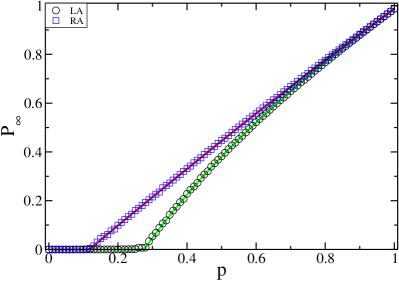
Figure 1: (Color online) Sizes of giant component, $P_{\infty}(p)$, as a function of $p$ for $\lambda_{1}=4$, $\lambda_{2}=12$ and $\alpha=0.7$. Here solid lines are theoretical predictions, from Eq. (13) for RA (red line) and Eq. (20) for LA (green line), and symbols are simulation results with network size $N=10^{4}$, where averages are taken over 10 realizations, under LA ($\bigcirc$) and RA ($\square$).

In order to determine $p_{c}$ explicitly, we first get $f_{c}$ from $f_{c}\equiv G^{-1}_{0}(p_{c})$, i.e., $f_{c}$ from $G_{0}(f_{c})=p_{c}$. Then from Eq. (19) $f_{c}$ must also satisfy $G^{{}^{\prime\prime}}_{0}(f_{c})=G^{{}^{\prime}}_{0}(1)$. In the general case, $p_{c}$ and $P_{\infty}$ must be obtained by solving numerically Eqs. (19) and (20). In certain limiting cases, however, one can derive explicit analytical expressions for $p_{c}$ that yield more physical insight. An example of a specific case is given in the next subsection.

II.1.1 Analytic solution of $p_{c}$ for bi-Poisson distribution with $\lambda_{2}=2\lambda_{1}$

For a bi-Poisson distribution, using its generating function and $G_{0}(f_{c})=p_{c}$, $f_{c}$ and $p_{c}$ satisfy the relation

$$G_{0}(f_{c})=\alpha[e^{(f_{c}-1)}]^{\lambda_{1}}+(1-\alpha)[e^{(f_{c}-1)}]^{\lambda_{2}}=p_{c}.$$ (21)

Assuming $\lambda_{2}=2\lambda_{1}$, we denote $e^{\lambda_{1}(f_{c}-1)}=y$ such that Eq. (21) reduces to $\alpha y+(1-\alpha)y^{2}=p_{c}$, which, for $\alpha\neq 1$, is a quadratic equation of $y$ and its positive solution is

$$y=\frac{\sqrt{\alpha^{2}+4p_{c}(1-\alpha)}-\alpha}{2(1-\alpha)}.$$ (22)

Plugging $f_{c}$ into Eq. (19) we get another quadratic equation of $y$,

$$\alpha\lambda_{1}^{2}y+(1-\alpha)\lambda_{2}^{2}y^{2}=\alpha\lambda_{1}+(1-\alpha)\lambda_{2},$$ (23)

for which the physical solution of $y$ is

$$y=\frac{\sqrt{\alpha^{2}\lambda_{1}^{4}+4(1-\alpha)\lambda_{2}^{2}[\alpha(\lambda_{1}-\lambda_{2})+\lambda_{2}]}-\alpha\lambda_{1}^{2}}{2(1-\alpha)\lambda_{2}^{2}}.$$ (24)

Because $f_{c}=ln(y)/\lambda_{1}+1$, to obtain $p_{c}$ we need to equate Eqs. (22) and (24). Thus we obtain

$$p_{c}=\frac{1}{64(1-\alpha)}[\beta+6\alpha\sqrt{\alpha^{2}+\beta}-6\alpha^{2}],$$ (25)

where $\beta=\frac{16(1-\alpha)(2-\alpha)}{\lambda_{1}}$. We use the relation of $\lambda_{2}=2\lambda_{1}$ for simplification. Plugging $\alpha=0$ into Eq. (25), we get $p_{c}={1}/{\lambda_{2}}$ as found in Ref. (Shao et al., 2015). For $\alpha\rightarrow 1$, employing the L’Hôpital rule we also get $\lim_{\alpha\to 1}p_{c}={1}/{\lambda_{1}}$, as found in the pure Poisson distribution described above.

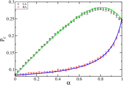
Figure 2: (Color online) Percolation thresholds $p_{c}$ of a single bi-Poisson network as a function of $\alpha$ under LA and RA with $\lambda_{1}=4$, $\lambda_{2}=12$. Here solid lines are theoretical predictions, from Eq. (11) for RA (blue line) and Eq. (19) for LA (green line) and symbols ($\square$ for RA and $\bigcirc$ for LA) with error bars are simulation results with network size of $N=10^{4}$ nodes, where averages and standard deviations are taken over 20 realizations.

It is impossible to derive $p_{c}$ explicitly for a Gaussian distribution. Even for a bi-Poisson distribution, other than special cases such as the one discussed above, deriving $p_{c}$ is also impossible because it requires solving first $f_{c}=G^{-1}_{0}(p_{c})$, i.e., $f_{c}$ from Eq. (21), which could be viewed as $\alpha y^{\lambda_{1}}+(1-\alpha)y^{\lambda_{2}}=p_{c}$, a polynomial equation of $y=e^{(f_{c}-1)}$. Because we also consider the cases of $\lambda_{2}>\lambda_{1}\geqslant 4$ using the Abel-Ruffini theorem, there is no general algebraic solution to the above equation except in some special cases. Hence we use the Newton method to solve $p_{c}$ and $P_{\infty}$ numerically.

II.2 Results

To test the analytical predictions above we conduct numerical calculations of analytic expressions, and compare the results with the simulation results on single networks with degrees following both bi-Poisson distributions and Gaussian distributions under both LA and RA. All the simulation results are obtained for networks of $N=10^{4}$ nodes.

II.2.1 Single bi-Poisson networks

Figure 1 shows the giant component $P_{\infty}(p)$ as a function of the occupation probability $p$ under LA and RA. Note that $p_{c}$ is larger for LA than for RA. The simulation results agree with the theoretical results obtained from Eqs. (13) and (20), and there is second-order percolation transition behavior in both attack scenarios. Note that when $\alpha=0$ or $1$, i.e., when node degrees follow a pure Poisson distribution as reported in Ref. Shao et al. (2015), the networks have the same critical value of $p_{c}$ under LA and RA and the same dependence of $P_{\infty}(p)$ on $p$. However when $\alpha=0.7$, $p_{c}(LA)>p_{c}(RA)$, indicating that the network is more fragile under LA than under RA, and that the giant components exhibit different behavior.

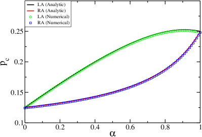
Figure 3: (Color online) Comparison between numerical results (symbols) and the analytic results (solid lines) for bi-Poisson distribution with $\lambda_{1}=4$ and $\lambda_{2}=8$. Note that they agree with each other well. Here, all the analytic results are obtained from Eq. (11) for RA (red line) and Eq. (25) for LA (black line) and the numerical results are attained by employing Newton’s Method on Eqs. (11) and (19) respectively.

Figure  2 shows how the broadness of the distribution, tuned by changing $\alpha$ with fixed $\lambda_{1}$ and $\lambda_{2}$, influences the robustness of the network under LA and RA. The solid lines are the numerical results obtained from the Newton method and the symbols with error bars are the simulation results. Note that only when $\alpha=0$ and $\alpha=1$ does $p_{c}(LA)=p_{c}(RA)$. In all other cases $p_{c}(LA)>p_{c}(RA)$, indicating that the network is always more vulnerable under LA than under RA if the degree distribution is bi-Poissonian. Note also that $p_{c}(LA)$ peaks at $\alpha=0.79$.

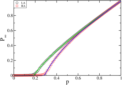
Figure 4: (Color online) Sizes of giant component as a function of $p$ of a single Gaussian network with $\mu=4$ and $\sigma^{2}=2$. Here solid lines are theoretical results, from Eq. (13) for RA (blue line) and Eq. (20) for LA (green line) and symbols are simulation results obtained from network size of $N=10^{4}$ where averages are taken over 10 realizations under LA ($\bigcirc$) and RA ($\square$).

For the special case of $\lambda_{2}=2\lambda_{1}$, we compare the analytical values of $p_{c}$ from Eqs. (11) and (25) using $\lambda_{1}=4$ and $\lambda_{2}=8$ with results obtained from the Newton method (see Fig. 3). For this combination of average degrees, $p_{c}(LA)$ peaks at $\alpha=0.91$. Note that the results agree, indicating that the Newton method produces satisfactory results and therefore, in the general case in which $\lambda_{2}\neq 2\lambda_{1}$ and in the cases of Gaussian distribution, it can be used to get $p_{c}(LA)$.

II.2.2 Single Gaussian Networks

Figure 4 shows the giant component $P_{\infty}(p)$ as a function of the occupation probability $p$ under LA and RA respectively for a single network with a Gaussian degree distribution. Note that the simulation results and the theoretical results obtained from Eqs. (13) and (20) agree, and that second-order phase transition behavior is present in both attack scenarios. Note also that $\mu=4$ and $\sigma^{2}=2$, and thus $p_{c}(LA)<p_{c}(RA)$, which indicates that the network is more robust under LA than under RA for this particular distribution.

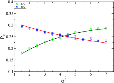
Figure 5: (Color online) Percolation thresholds $p_{c}$ as a function of $\sigma^{2}$ of networks with Gaussian degree distribution under LA and RA with $\mu=4$. Here solid lines are theoretical predictions, from Eq. (12) for RA (red line) and Eq. (19) for LA (black line) and symbols ($\square$ for RA and $\bigcirc$ for LA) with error bars are simulation results with network size of $N=10^{4}$ nodes, where averages and standard deviations are taken over 20 realizations. It is shown here that as $\sigma^{2}$ increases $p_{c}(LA)$ increases whereas $p_{c}(RA)$ decreases simultaneously and they intersect each other around $\sigma^{2}\approx\mu=4$.

We fix $\mu$ and find that when the Gaussian distribution gets broader, i.e., when $\sigma$ increases, $p_{c}(RA)$ decreases, but that $p_{c}(LA)$ increases with $\sigma$ (see Fig. 5). Note that when $\sigma^{2}<\mu$, $p_{c}(LA)<p_{c}(RA)$, and that the opposite is true when $\sigma^{2}>\mu$. Note also that when $\sigma^{2}\approx\mu$ there is a crossing point with $p_{c}(RA)\approx p_{c}(LA)$, which is analogous to a Poisson ER network with the same mean and variance and the robustness of the network under both LA and RA is the same, as reported in Ref. Shao et al. (2015).

Figure 6 shows a plot of $\sigma^{2}$ as a function of $\mu$ when this intersection point occurs, i.e., when $p_{c}(LA)=p_{c}(RA)$. Note that except for some minor deviations at small $\mu$ values, because $k\geq 0$ the Gaussian distribution is deformed, the region above the extrapolation curve corresponds to $p_{c}(LA)>p_{c}(RA)$, and the region below to $p_{c}(LA)<p_{c}(RA)$.

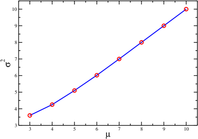
Figure 6: (Color online) $\sigma^{2}$ as a function of $\mu$ at the intersection point where $p_{c}(LA)=p_{c}(RA)$ for single networks where degrees follow a Gaussian distribution.

III RA and LA on Fully Interdependent Networks

III.1 Theory

We apply the formalism of RA on fully interdependent networks introduced in Ref. Buldyrev et al. (2010). Specifically, we consider two networks $A$ and $B$ with the same number of nodes $N$. Within each network the nodes are randomly connected with degree distributions $P_{A}(k)$ and $P_{B}(k)$ respectively. Every node in network $A$ depends on a random node in network $B$, and vice versa. We also assume that if a node $i$ in network $A$ depends on a node $j$ in network $B$ and node $j$ depends on node $l$ in network $A$, then $l=i$, which rules out the feedback condition Gao et al. (2013). This full interdependency means that every node $i$ in network $A$ has a dependent node $j$ in network $B$, and if node $i$ fails node $j$ will also fail, and vice versa.

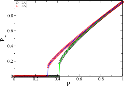
Figure 7: (Color online) Sizes of the mutually connected giant component of the fully interdependent bi-Poisson networks as a function of $p$ for $\lambda_{1}=4$, $\lambda_{2}=12$ and $\alpha=0.5$. Here solid lines are theoretical predictions, from Eq. (26) for RA (blue line) and similarly for LA (green line), and symbols are simulation results with network size $N=10^{4}$, where averages are taken over 10 realizations, under LA ($\bigcirc$) and RA ($\square$).

(I) Random Attack: We begin by randomly removing a fraction $1-p$ of nodes and their links in network $A$. All the nodes in network $B$ that are dependent on the removed nodes in network $A$ are also removed along with their connectivity links. As nodes and links are sequentially removed, each network begin to break down into connected components. Due to interdependency, the removal process iterates back and forth between the two networks until they fragment completely or produce a mutually connected giant component with no further disintegration. As in Ref. Buldyrev et al. (2010) we introduce the function $g_{A}(p)=1-G_{A0}[1-p(1-f_{A})]$, which is the fraction of nodes that belong to the giant component of network $A$, where $f_{A}$ is a function of $p$ that satisfies the transcendental equation $f_{A}=G_{A1}[1-p(1-f_{A})]$. Similar equations exist for network $B$. When the system of interdependent networks stops disintegrating, the fraction of nodes in the mutual giant component is $P_{\infty}$, satisfying

$$P_{\infty}=xg_{B}(x)=yg_{A}(y),$$ (26)

where $x$ and $y$ satisfy

$$x=pg_{A}(y),y=pg_{B}(x).$$ (27)

Excluding the trivial solution $x=0,y=0$ to the equation set above, we combine them into a single equation by substitution and obtain,

$$x=g_{A}[g_{B}(x)p]p.$$ (28)

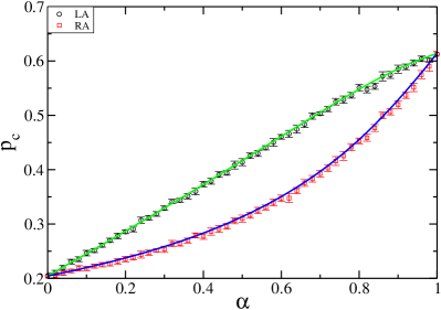
Figure 8: (Color online) Percolation thresholds $p_{c}$ of the fully interdependent bi-Poisson networks with $\lambda_{1}=4$, $\lambda_{2}=12$ as a function of $\alpha$ under LA and RA. Here solid lines are theoretical predictions, from Eq. (29) for RA (blue line) and similarly for LA (green line) and symbols ($\square$ for RA and $\bigcirc$ for LA) with error bars are simulation results with network size of $N=10^{4}$ nodes, where averages and standard deviations are taken from 20 realizations. When $\alpha$ is not 1 or 0, $p_{c}(LA)$ is always larger than $p_{c}(RA)$.

A nontrivial solution emerges in the critical case ($x=x_{c},p=p_{c}$) by equating the derivatives of both sides of Eq. (28) with respect to $x$

$$1=p^{2}\frac{dg_{A}[pg_{B}(x)]}{dx}\frac{dg_{B}(x)}{dx}\vline_{x=x_{c},p=p_{c}}$$ (29)

which, together with Eq. (27), gives the solution for $p_{c}$ and the critical size of the mutually connected component, $P_{\infty}(p_{c})=x_{c}g_{B}(x_{c})$.

(II) Localized Attack: When LA is performed on the one-to-one fully interdependent networks $A$ and $B$ described above, we can find an equivalent random network $E$ with generating function $G_{E0}(x)$ such that after a random attack in which $1-p$ nodes in network $E$ are removed, the generating function of the degree distribution of the remaining network is the same as $G_{p0}(x)$ (with the substitution of $G_{0}(x)$ by $G_{A0}(x)$). Then the LA problem on networks $A$ and $B$ can be mapped to a RA problem on networks $E$ and $B$. By using $G_{E0}(1-p+px)=G_{p0}(x)$ and from Eq. (15) we have

$$G_{E0}(x)=\frac{1}{G_{A0}(f)}G_{A0}[f+\frac{G^{{}^{\prime}}_{A0}(f)}{G^{{}^{\prime}}_{A0}(1)G_{A0}{(f)}}(x-1)].$$ (30)

Thus by mapping the LA problem on interdependent networks $A$ and $B$ to a RA problem on a transformed pair of interdependent networks $E$ and $B$, we can apply the mechanism of RA on interdependent networks to solve $p_{c}$ and $P_{\infty}(p)$ under LA.

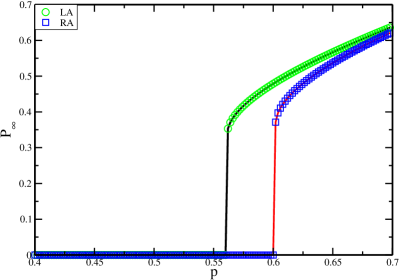
Figure 9: (Color online) Sizes of mutual giant component of the fully interdependent Gaussian networks as a function of $p$ with $\mu=4$ and $\sigma^{2}=2$. Here solid lines are theoretical predictions, from Eq. (26) for RA (red line)and similarly for LA (black line), and symbols are simulation results with network size $N=10^{4}$, where averages are taken over 10 realizations, under LA ($\bigcirc$) and RA ($\square$).

Note that for pure Poisson distributions, $f\equiv G^{-1}_{A0}(p)=\frac{ln(p)}{\lambda}+1$, and that by substituting $f$ into Eq. (30) we get $G_{E0}(x)=G_{A0}(x)$. Thus we find that pure Poisson distributions have exactly the same percolation properties for fully interdependent networks under LA as those under RA, as found in Ref. (Buldyrev et al., 2010). Because the extreme complexity of the above equations makes it difficult to obtain explicit expressions for $p_{c}$ and $P_{\infty}(p)$ except when degree distributions are simple, we resort to numerical calculations in general.

III.2 Results

III.2.1 Fully interdependent networks with bi-Poisson degree distribution

We start with two fully interdependent networks in which the degrees both follow the same bi-Poisson distribution and carry out a RA on one of the networks, initiating a cascading failure process that will continue until equilibrium is reached. We then do the same procedure with the same set-up but this time using a LA to initiate the cascading failure process. Figure 7 shows the size of the giant component $P_{\infty}(p)$ of the system as a function of the occupation probability $p$ under LA and under RA. Note that in both RA and LA scenarios the simulation results and the theoretical results obtained from Eq. (26) agree, indicating that our strategy of finding an equivalent network under LA works. The first-order phase transition that occurs in both attack scenarios indicates that the interdependency of the system makes it much more vulnerable to attack than single networks. When $\alpha=0.5$ the system is more fragile under LA than under RA with $p_{c}(LA)>p_{c}(RA)$, and the giant components exhibit different behaviors.

Figure 8 shows how the broadness of the distribution, tuned by changing $\alpha$ with fixed $\lambda_{1}$ and $\lambda_{2}$, influences the robustness of the network under both LA and RA. Solid lines are numerical results using the Newton method on Eq. (29) and symbols with error bars are simulation results. Note that only when $\alpha=0$ and $\alpha=1$ is $P(k)$ reduced to a pure Poisson, and we have $p_{c}(LA)=p_{c}(RA)=2.4554/\left\langle k\right\rangle$, as in Ref. Buldyrev et al. (2010). When $\alpha$ deviates from 0 or 1, i.e., when $P(k)$ deviates from a pure Poisson distribution and takes the form of a bi-Poisson distribution, $p_{c}(LA)>p_{c}(RA)$, indicating that the system is more vulnerable under LA than under RA.

Figure 10: (Color online) Percolation thresholds $p_{c}$ as a function of $\sigma^{2}$ of the fully interdependent Gaussian networks under LA and RA with $\mu=4$. Here solid lines are theoretical predictions, from Eq. (29) for RA (red line) and similarly for LA (black line) and symbols ($\square$ for RA and $\bigcirc$ for LA) with error bars are simulation results with network size of $N=10^{4}$ nodes, where averages and standard deviations are taken from 20 realizations. It is seen here that as $\sigma^{2}$ increases $p_{c}(LA)$ increases and $p_{c}(RA)$ has a tendency to decrease. As $\sigma^{2}$ approaches the value of $\mu$, $p_{c}(LA)\approx p_{c}(RA)$, which is manifested by the intersection point shown here.

III.2.2 Fully interdependent networks with Gaussian degree distribution

We construct two fully interdependent networks in which the degrees in each network follow the same Gaussian distribution and carry out a RA on one of the networks to initiate a cascading failure process that will continue until it reaches a steady state. We repeat the action, but this time using a LA. Figure 9 shows the sizes of the giant component $P_{\infty}(p)$ as a function of the occupation probability $p$ under both LA and RA. Note that simulation results and the theoretical results obtained from Eq. (26) agree. When $\mu=4$ and $\sigma^{2}=2$ the system is more fragile under LA than under RA with $p_{c}(LA)<p_{c}(RA)$, and the giant components exhibit different behaviors.

If we fix $\mu$, when the Gaussian distribution gets broader, i.e., when $\sigma$ increases, analogous to what we find in a single Gaussian network, the critical $p_{c}$ behavior of the system differs under LA from that under RA. Figure 10 shows the effect of $\sigma$ on $p_{c}$ in the fully interdependent Gaussian networks. When $\sigma^{2}<\mu$, $p_{c}(LA)<p_{c}(RA)$, and the opposite occurs when $\sigma^{2}>\mu$. The intersection point in Fig. 10 is located near $\sigma^{2}\approx\mu$, similar to that in Poisson distribution networks. Thus the system behaves the same under LA as under RA, confirming the results presented in the previous subsection. Note that our results show that in both attack scenarios, the interdependency of the system makes it much more vulnerable to RA and LA compared to single networks (compare Fig. 10 to Fig. 5).

IV Conclusions

In summary, we show that a LA on interdependent networks can be mapped to a RA problem by transforming the network under initial attack. We also show how the broadness of the degree distribution affects the robustness of networks against RA and LA respectively. We show that, in general, as the degree distribution broadens the network becomes more vulnerable to LA than RA. This finding holds for both single networks and interdependent networks.

References

- Watts and Strogatz (1998) D. J. Watts and S. H. Strogatz, Nature 393, 440 (1998).
- Albert et al. (2000) R. Albert, H. Jeong, and A.-L. Barabási, Nature 406, 378 (2000).
- Cohen et al. (2000) R. Cohen, K. Erez, D. Ben-Avraham, and S. Havlin, Phys. Rev. Lett. 85, 4626 (2000).
- Callaway et al. (2000) D. S. Callaway, M. E. Newman, S. H. Strogatz, and D. J. Watts, Phys. Rev. Lett. 85, 5468 (2000).
- Albert and Barabási (2002) R. Albert and A.-L. Barabási, Rev. Mod. Phys. 74, 47 (2002).
- Newman (2003) M. E. Newman, SIAM Rev. 45, 167 (2003).
- Song et al. (2005) C. Song, S. Havlin, and H. A. Makse, Nature 433, 392 (2005).
- Caldarelli and Vespignani (2007) G. Caldarelli and A. Vespignani, Large scale structure and dynamics of complex networks: from information technology to finance and natural science, vol. 2 (World Scientific, 2007).
- Rosato et al. (2008) V. Rosato et al., Int. J. Crit. Infrastruct. 4, 63 (2008).
- Arenas et al. (2008) A. Arenas, A. Díaz-Guilera, J. Kurths, Y. Moreno, and C. Zhou, Physics Reports 469, 93 (2008).
- Cohen and Havlin (2010) R. Cohen and S. Havlin, Complex networks: structure, robustness and function (Cambridge University Press, 2010).
- Newman (2010) M. Newman, Networks: An Introduction (Oxford University Press, 2010).
- Li et al. (2010) G. Li et al., Phys. Rev. Lett. 104, 018701 (2010).
- Schneider et al. (2011) C. M. Schneider et al., Proc. Natl. Acad. Sci. 108, 3838 (2011).
- Bashan et al. (2012) A. Bashan et al., Nature Commun. 3, 702 (2012).
- Dorogovtsev and Mendes (2013) S. N. Dorogovtsev and J. F. Mendes, Evolution of networks: From biological nets to the Internet and WWW (Oxford University Press, 2013).
- Ludescher et al. (2013) J. Ludescher et al., Proc. Natl. Acad. Sci. 110, 11742 (2013).
- Yan et al. (2013) X. Yan, Y. Fan, Z. Di, S. Havlin, and J. Wu, PloS one 8, e69745 (2013).
- Boccaletti et al. (2014) S. Boccaletti et al., Physics Reports 544, 1 (2014).
- Li et al. (2015) D. Li et al., Proc. Natl. Acad. Sci. 112, 669 (2015).
- Shao et al. (2015) S. Shao, X. Huang, H. E. Stanley, and S. Havlin, New J. Phys. 17, 023049 (2015).
- Berezin et al. (2015) Y. Berezin, A. Bashan, M. M. Danziger, D. Li, and S. Havlin, Scientific Reports 5, 8934 (2015).
- Buldyrev et al. (2010) S. V. Buldyrev, R. Parshani, G. Paul, H. E. Stanley, and S. Havlin, Nature 464, 1025 (2010).
- Huang et al. (2011) X. Huang et al., Phys. Rev. E 83, 065101 (2011).
- Peixoto and Bornholdt (2012) T. P. Peixoto and S. Bornholdt, Phys. Rev. Lett. 109, 118703 (2012).
- Baxter et al. (2012) G. Baxter, S. Dorogovtsev, A. Goltsev, and J. Mendes, Phys. Rev. Lett. 109, 248701 (2012).
- Dong et al. (2012) G. Dong, J. Gao, L. Tian, R. Du, and Y. He, Phys. Rev. E 85, 016112 (2012).
- Bashan et al. (2013) A. Bashan, Y. Berezin, S. V. Buldyrev, and S. Havlin, Nature Physics 9, 667 (2013).
- Radicchi and Arenas (2013) F. Radicchi and A. Arenas, Nature Physics 9, 717 (2013).
- Valente et al. (2004) A. X. Valente, A. Sarkar, and H. A. Stone, Phys. Rev. Lett. 92, 118702 (2004).
- Tanizawa et al. (2006) T. Tanizawa, G. Paul, S. Havlin, and H. E. Stanley, Phys. Rev. E 74, 016125 (2006).
- Pennock et al. (2002) D. M. Pennock, G. W. Flake, S. Lawrence, E. J. Glover, and C. L. Giles, Proc. Natl. Acad. Sci. 99, 5207 (2002).
- Newman (2002) M. E. Newman, Phys. Rev. E 66, 016128 (2002).
- Shao et al. (2009) J. Shao, S. V. Buldyrev, L. A. Braunstein, S. Havlin, and H. E. Stanley, Phys. Rev. E 80, 036105 (2009).
- Gao et al. (2013) J. Gao et al., Phys. Rev. E 88, 062816 (2013).