Relaxation in $N$-body simulations of spherical systems

Abstract

I present empirical measurements of the rate of relaxation in $N$-body simulations of stable spherical systems and distinguish two separate types of relaxation: energy diffusion that is largely independent of particle mass, and energy exchange between particles of differing masses. While diffusion is generally regarded as a Fokker-Planck process, it can equivalently be viewed as the consequence of collective oscillations that are driven by shot noise. Empirical diffusion rates scale as $N^{-1}$ in inhomogeneous models, in agreement with Fokker-Planck predictions, but collective effects cause relaxation to scale more nearly as $N^{-1/2}$ in the special case of a uniform sphere. I use four different methods to compute the gravitational field, and a 100-fold range in the numbers of particles in each case. I find the rate at which energy is exchanged between particles of differing masses does not depend at all on the force determination method, but I do find the energy diffusion rate is marginally lower when a field method is used. The relaxation rate in 3D is virtually independent of the method used because it is dominated by distant encounters; any method to estimate the gravitational field that correctly captures the contributions from distant particles must also capture their statistical fluctuations and the collective modes they drive.

1 Introduction

The topic of relaxation driven by stellar encounters in star systems has a long and distinguished history (e.g. Chandrasekhar, 1941; Binney & Tremaine, 2008) and has important implications for the evolution of star clusters (Spitzer, 1987) and of active galactic nuclei (Merritt, 2013). However, it is widely believed that relaxation through star-star encounters occurs at a negligible rate in the bulk of galaxies, and therefore $N$-body simulations of galaxies should mimic this collisionless property. The study presented here focuses on just one small aspect of the general problem of relaxation in simulations.

Although the computational power available to simulators has risen steadily over time, calculations with billions of particles are still not routinely possible and most simulations employ fewer, more massive particles. A rough estimate of the relaxation time $t_{\rm relax}$ in a simulation of $N$ equal mass particles is (e.g. Binney & Tremaine, 2008)

$$t_{\rm relax}/t_{\rm cross}\sim 0.1N/\ln N,$$ (1)

with $t_{\rm cross}$ being a typical crossing time. This, as other more precise expressions for Fokker-Planck diffusion, contains the Coulomb logarithm that arises from integration over impact parameters, implying that every decade of impact parameter makes an equal contribution to the integral. It should be noted that the approximate formula (1) applies for pressure-supported systems, not discs (Sellwood, 2013), and neglects collective effects. Furthermore, it was derived for nominally point mass particles, since the argument of the logarithm comes from the ratio of the system half-mass radius to the scale on which scattering causes large deflections, whose contributions would otherwise be overestimated. It therefore reflects spatial resolution, which is usually determined by other factors, such as particle softening or grid resolution in $N$-body codes. Therefore, $t_{\rm relax}$ should be simply proportional to $N$ when resolution is held fixed.

Numerical methods used to compute the gravitational field in simulations that aspire to be collisionless fall into three broad categories. The most popular direct method is some type of tree code (e.g. Barnes & Hut, 1986; Springel, 2005) that effectively sums the attraction of every particle pair, with a softening kernel to limit the magnitude of the acceleration at short range. The far more efficient (Sellwood, 2014) particle-mesh methods (PM, e.g. Hockney & Eastwood, 1981) determine the gravitational field on a raster of points that has some appropriate geometry; forces at the actual particle positions are computed by interpolation between grid points. Finally, the least popular are field methods (e.g. Clutton-Brock, 1972; Hernquist & Ostriker, 1992) that expand the density and potential in a basis set of functions that should be chosen such that truncating the expansion at low order yields an adequate approximation to the field.

Weinberg, in a series of papers (Weinberg, 1999; Holley-Bockelmann, Weinberg & Katz, 2005; Weinberg & Katz, 2007a, b) has argued that field methods are inherently superior to other $N$-body methods in their ability to hide the lumpiness of the potential from a set of point masses. In particular, Weinberg & Katz (2007b) assert that field methods have “relaxation times … orders of magnitude longer” than in tree codes. This claim was based on a lengthy calculation using Hamiltonian mechanics that I review below.

Since a well-chosen basis can yield an adequate approximation to the total field from a small number of terms, it may seem reasonable to expect the resulting potential to be smoother than that computed by other methods. However, this argument is beguiling for the following reasons. Only the lowest order monopole term has a large value about which shot noise fluctuations are small, while the amplitudes of the aspherical terms, which are oscillatory, depend on the almost-complete cancellation of the $N$ contributions, and are entirely noise-driven in a spherical model, for example. It is also true that the number of values that define the potential in PM codes is $n_{\rm grid}$ and, since each mesh point typically hosts $\sim N/n_{\rm grid}$ particles, each separate value will be subject to a greater degree of shot noise. In direct methods, there are $N$ separate contributions to the field. But note that the potential is the double integral of the density; in effect, the potential kernel, which is monotonic and has infinite range, implies the field at each point is the sum of contributions from all the sources. Thus potential variations are far smoother than could be supported by an arbitrary function defined by the same number of values.

Hernquist & Barnes (1990, hereafter HB90) used a King model for an experimental comparison between the relaxation rates in simulations when the gravitational field was determined by three different methods, and Hernquist & Ostriker (1992) extended their results to include a field method. They found that the rate of energy diffusion of particles was only mildly affected by the method used. While their evidence was quite strong, they generally employed only 4096 particles and gravity softening spoiled the equilibrium of some of their initial models. Sellwood (2008) showed that grid and field methods performed equally well in the specific problem of bar-halo friction.

Here I present a more general study of fully self-consistent equilibrium spheres that uses two distinct measures of the “relaxation” rate: the energy diffusion rate reported by HB90, and a measure of the rate of energy exchange between particle species of differing masses. The former measure includes all sources of relaxation, especially collective effects, while the latter is a more direct consequence of two-body encounters.

2 Models

In order to illustrate the importance of collective effects, I here report measurements in three different mass models. All three are spheres with ergodic (isotropic) distribution functions (DFs) that are therefore stable equilibria.

The mass models are:

1. Hernquist model Hernquist (1990) developed a simple spherical model having the centrally cusped density profile

   $$\rho(r)={Ma\over 2\pi r(r+a)^{3}},$$ (2)

   which has the potential $\Phi(r)=-GM/(a+r)$. Here $a$ is a length scale and $M$ the finite total mass integrated to infinity. Hernquist also gave the equilibrium isotropic DF for this density and potential. I truncate this model so that no particle has sufficient energy to stray beyond $r=10a$, which causes the density profile to taper smoothly to zero at that radius, and discards $\sim 26$% of the mass, but leaves the density profile as given by eq. (2) over the range $0\leq r/a\la 5$.

2. Plummer sphere Plummer (1911) introduced one of the most widely used spherical mass models in astronomy. It has the cored density profile

   $$\rho(r)={3M\over 4\pi a^{3}}(1+x^{2})^{-5/2},$$ (3)

   where $x=r/a$ and $M$ is the total mass. The potential is $\Phi(r)=-(GM/a)(1+x^{2})^{-1/2}$, and the isotropic DF is that of a polytrope of index 5 (see BT08). Applying an energy truncation so that no particle passes outside $r=10a$ discards only $\sim 3.4$% of the mass in this model with its lower density envelope.

3. Uniform sphere with density $\rho_{0}=3M/(4\pi a^{3})$, where $a$ is the outer radius. Polyachenko & Shukhman (1979) give the isotropic DF for a homogeneous sphere with a sharp outer boundary. The harmonic potential in the interior of this unusual model implies that all particles have the same orbital frequencies; this model, therefore, affords a dramatic illustration of the role of collective effects.

In all cases, I employ two equally numerous sets of particles drawn from the DF: the masses of particles, $m_{i}=\mu_{i}m_{*}$ are such that those of one sample have $\mu_{i}=9$ and the other have $\mu_{i}=1$, and $m_{*}$ is chosen such that the combined density profile is that given by the above expressions. Debattista & Sellwood (2000, appendix A) describe an optimal method of drawing particle coordinates from a DF in such a way as to reduce shot noise in the distribution of energies. Sellwood (2014) reports results that show the material benefit of this strategy.

The models are evolved for 100 dynamical times, where $t_{0}=(a^{3}/GM)^{1/2}$, with a timestep of $0.02t_{0}$ for the uniform sphere and Plummer models. The basic step for the Hernquist model is $0.0125$ but time steps are increased, in this case only, by four successive factors of 2 at appropriate radii. I save the instantaneous energy of a representative set of particles ($2\times 10^{4}$ or all, whichever is the less) after every dynamical time.

3 Methods

I employ four different numerical methods to determine the gravitational field from the particles:

1. BHT A tree code that uses the scheme first proposed by Barnes & Hut (1986). I include dipole terms and particle groupings are opened when they subtend an angle $>\theta_{\rm max}=0.5$ radians. Forces are softened at short range only using the kernel advocated by Monaghan (1992), with $\epsilon=0.05a$ for the uniform sphere and $\epsilon=0.1a$ for the other two models.

2. S3D A spherical grid, which is a hybrid PM expansion method that expands the non-spherically symmetric part in surface harmonics on a set of spherical shells (McGlynn, 1984; Sellwood, 2003). Force discontinuities, which arise when particle radii cross, are eliminated by adopting linear interpolation between radial shells. I tabulate the expansion coefficients at 100 logarithmically spaced radii, and expand in azimuth up to $l_{\rm max}=8$.

3. SFP A field method that employs a biorthonormal set of basis functions (Clutton-Brock, 1972; Hernquist & Ostriker, 1992), which I name SFP (for smooth field-particle) but is also known as SCF. I expand in azimuth up to $l_{\rm max}=8$ and employ radial functions up to $n_{\rm max}=10$. I use this method for the Plummer and Hernquist models only.

4. C3D I do not use the SFP method for the uniform sphere, but employ a PM method that uses 3D Cartesian grid (James, 1977), and I set $a=50$ mesh spaces. The grid has $129^{3}$ points, except for the lowest $N$ case where it was $257^{3}$ points in order to allow plenty of room for expansion of the particle distribution. Linear interpolation results in the inter-particle force given in Sellwood & Merritt (1994, appendix), which is well approximated by cubic density kernel with $\epsilon\approx 1.8$ grid spaces (Sellwood, 2014).

More details of all these methods are given in the on-line manual (Sellwood, 2014).

The choices of numerical parameters in each case are somewhat arbitrary, but values are typical of those used in practice and are not varied as the particle number is changed. The rate of relaxation will depend only weakly on spatial resolution, since only short range scattering is affected by changes to the softening length, for example, leading to a slight change in the value of the Coulomb logarithm.

Truncating the expansion at low order in field methods smooths the mass distribution, and more aggressive truncation will give rise to a smoother potential, which must reduce the relaxation rate; e.g. in the extreme case of a single term, the particles will be moving in an almost fixed potential, and no evolution and little relaxation could occur. Since the purpose of simulations is to compute the self-consistent evolution as the density changes, I include sufficient terms to be able to follow changes that might be expected in an evolving model.

The tree code uses explicit particle softening, while short-range forces are implicitly smoothed in the Cartesian grid. These methods therefore do not yield the exact Newtonian potential of the mass distribution. In order to ensure that the initial model is in equilibrium in the tree code, I use the largest $N$ simulation of each type to tabulate the difference between the spherically averaged central attraction of the particles at $t=0$ and the analytic central attraction at a 1D array of points; I then interpolate from this table a supplementary central attraction that is added to the tree-determined force on each particle before its motion is advanced. I use a similar procedure for the 3D Cartesian grid, but in order to avoid shot noise in the (very small) permanent part of central attraction, the numerical force is computed from a smooth density distribution assigned to the grid. These generally small corrections are not needed for S3D or SFP methods.

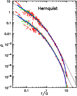
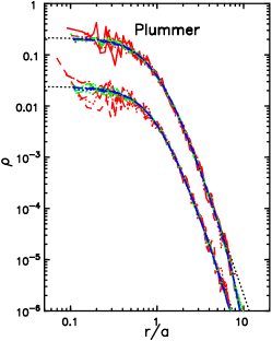
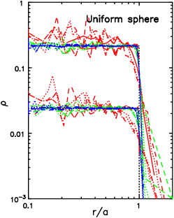
Figure 1: The final density profiles (coloured lines) measured from the different particle species that, in all 27 simulations, contribute 10% and 90% of the total density as indicated by the two groups of lines. In each panel, the colour indicates the number of particles: red is for $N=4\times 10^{3}$, green is for $N=4\times 10^{4}$ and blue is for $N=4\times 10^{5}$. The different methods for computing the field are distinguished by the line styles: solid is for S3D, dotted is for BHT, and dashed is for either SFP (Hernquist and Plummer) or C3D (uniform sphere). The black dotted curves indicate the expected density profile of each mass species; no particles in the left and middle panels started with enough energy to pass beyond $r=10a$.

With these fixed correction terms in C3D and BHT, and with a coordinate centre for the S3D and SFP methods, it is important to ensure that the initial set of particles is at rest and centred in this coordinate frame. After creating the initial set of particles, I therefore adjust the positions and speeds by a small amount to ensure the centre of mass is at the coordinate centre and the model has no net momentum. An alternative strategy that would achieve the same outcome would be to shift the grid (or expansion) centre at frequent intervals. I also experimented with inserting mirror pairs of particles having coordinates $(\;\kern-2.5pt\hbox{$\mit x$}\kern-5.2778pt\kern 0.50003pt\hbox{$\mit x$}\kern-5.2778pt\kern-0.24994pt\raise 0.43304pt\hbox{$\mit x$},\;\kern-2.5pt\hbox{$\mit v$}\kern-5.2778pt\kern 0.50003pt\hbox{$\mit v$}\kern-5.2778pt\kern-0.24994pt\raise 0.43304pt\hbox{$\mit v$})$ and $(-\;\kern-2.5pt\hbox{$\mit x$}\kern-5.2778pt\kern 0.50003pt\hbox{$\mit x$}\kern-5.2778pt\kern-0.24994pt\raise 0.43304pt\hbox{$\mit x$},-\;\kern-2.5pt\hbox{$\mit v$}\kern-5.2778pt\kern 0.50003pt\hbox{$\mit v$}\kern-5.2778pt\kern-0.24994pt\raise 0.43304pt\hbox{$\mit v$})$, in a step towards a quiet start, but this strategy had the undesirable (for this study) effects of eliminating any lop-sided, and emphasizing the bi-symmetric, contributions to the total field.

The instantaneous energy of the $i$th particle is approximately

$${\cal E}_{i}=m_{i}E_{i}(t)=m_{i}\left[\Phi(\;\kern-2.5pt\hbox{$\mit x$}\kern-5.2778pt\kern 0.50003pt\hbox{$\mit x$}\kern-5.2778pt\kern-0.24994pt\raise 0.43304pt\hbox{$\mit x$}_{i})+\textstyle{1\over 2}v_{i}^{2}\right],$$ (4)

where $E_{i}$ is the specific energy of the particle, or energy per unit mass, $\Phi$ is the estimated gravitational potential at the particle position, $\;\kern-2.5pt\hbox{$\mit x$}\kern-5.2778pt\kern 0.50003pt\hbox{$\mit x$}\kern-5.2778pt\kern-0.24994pt\raise 0.43304pt\hbox{$\mit x$}_{i}(t)$, and $v_{i}(t)$ is the scalar speed of the particle. This definition is exact only for a particle of infinitesimal mass, since a finite mass particle contributes to $\Phi$. The energy required to disperse a system of gravitating particles, the total energy, is ${\cal E}_{\rm tot}=T+W$, where $T=\sum_{i}{1\over 2}m_{i}v_{i}^{2}$ and $W={1\over 2}\sum_{i}m_{i}\Phi(\;\kern-2.5pt\hbox{$\mit x$}\kern-5.2778pt\kern 0.50003pt\hbox{$\mit x$}\kern-5.2778pt\kern-0.24994pt\raise 0.43304pt\hbox{$\mit x$}_{i})$, and the $W$ term is halved because the summation over the $\Phi$ values includes every pair of particles twice. The total energy, defined this way is very well conserved in the simulations, whereas the sum of the energies (eq. 4), $\sum_{i}{\cal E}_{i}=T+2W$, is clearly not the total energy, and is not conserved.

In order to test for virial equilibrium of an $N$-body simulation, it is better to measure the virial of Clausius, $W_{c}\equiv\sum_{i}m_{i}\;\kern-2.5pt\hbox{$\mit x$}\kern-5.2778pt\kern 0.50003pt\hbox{$\mit x$}\kern-5.2778pt\kern-0.24994pt\raise 0.43304pt\hbox{$\mit x$}_{i}\cdot\;\kern-2.5pt\hbox{$\mit a$}\kern-5.00002pt\kern 0.50003pt\hbox{$\mit a$}\kern-5.00002pt\kern-0.24994pt\raise 0.43304pt\hbox{$\mit a$}_{i}$, since the inter-particle forces are not perfectly Newtonian, especially at short range. It is easy to show that $W_{c}=W$ for precisely inverse-square law accelerations. The particle distribution is in equilibrium when $2T=|W_{c}|$.

It is convenient to chose units such that $G=M=a=1$, so that the dynamical time $t_{0}=(a^{3}/GM)^{1/2}=1$, for example. A convenient scaling to physical units for the inhomogeneous models is to choose $a=3\;$kpc and $t_{0}=10\;$Myr, which implies $M=6\times 10^{10}\;$M_⊙ and velocities scale as $(GM/a)^{1/2}\simeq 293\;$km/s.

4 Results

Figure 1 shows the final ($t=100t_{0}$) density profiles in all 27 simulations. The three panels show the different mass models. Within each panel the curves drawn in red are from the lowest $N=4\times 10^{3}$, those in green employ $4\times 10^{4}$ particles, and those in blue $4\times 10^{5}$, with $N/2$ in each mass species so that the initial densities from each species differ by factors of nine, as shown. The field is determined on the S3D grid for the full-drawn curves, the BHT method for the dotted curves, while the dashed curves are from either the SFP, for the Hernquist and Plummer models, or C3D for the uniform sphere.

The density profiles of the models evolve insignificantly for the largest $N$ (blue curves), confirming that the models are stable equilibria. As expected, relaxation drives the greatest changes in the simulations with the smallest $N$ (red curves) where, in a few cases, there are hints of some slight segregation of the particles of different masses over the time interval computed.

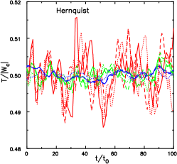
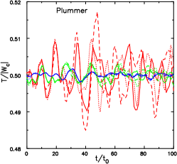
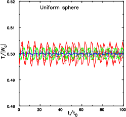
Figure 2: The time evolution of the virial ratio in all 27 simulations. As for Fig. 1, the colour indicates the number of particles while the different methods for computing the field are distinguished by the line styles.

4.1 Collective modes

Figure 2 shows the time evolution of the virial ratio, $T/|W_{c}|$ in all 27 simulations reported here. The three panels show the different mass models and the colours and line styles are used to distinguish the particle number and field determination method, as in Fig. 1.

It is clear from Figure 2 that the virial ratio $T/|W_{c}|$ remains close to $1\over 2$ for the duration of all these simulations, and the fluctuations around this ratio are largest for the lowest $N$ (red curves) and smallest for the highest $N$ (blue curves). The fluctuations are aperiodic for the inhomogeneous models, but are periodic in the uniform sphere, where they have very nearly the same period, $2\pi t_{0}$, in all nine simulations. Furthermore, the initial behaviour of the curves for models with the same $N$ (colour) is very similar for the different field determination methods, because the models were set-up using particles having the same positions and velocities. The red curves diverge quite noticeably, but the blue curves for the SCF and S3D methods remain barely distinguishable to the end; a slightly different value of $W_{c}$ arises in the BHT code because the forces differ due to softening and corrective terms, which is the reason the dotted curves remain distinct, particularly in the Hernquist model.

It is helpful to think of these fluctuations as the consequences of collective modes that are driven by shot-noise in the finite number of particles, as was recognized long ago by Rostoker & Rosenbluth (1960) in the context of collisionless plasmas, and has been studied in gravitating systems by Weinberg (1998) and others. The simplifying concept here is to distinguish the ideal collisionless system, which has a set of neutral and/or damped modes, from the noise spectrum arising from the particles that excites the modes. In principle, this approach would enable the evolution to be calculated by perturbation theory. Naturally, such an analysis should not differ in its predictions from the direct evolution of an $N$-body system composed of equal mass particles, which is exactly what the simulations compute. The results presented below reveal that relaxation is largely independent of particle mass, indicating that global modes are the dominant relaxation mechanism even when not every particle has the same mass.

The amplitudes of the modes should scale with the shot noise, and the rms scatter in $T/|W_{c}|$ about the value 0.5 indeed scales approximately as $N^{-1/2}$. The modes have essentially the same frequency in the uniform sphere where they appear to be almost undamped. Modes in collisionless systems can be damped only through resonant exchanges between the mode and the particles, and conditions for resonant damping are highly unfavorable because all particles have the same frequencies in this harmonic potential.

The aperiodic fluctuations in the inhomogeneous models (left and middle panels) reflect the broader range of frequencies among the particles in these models. Collective oscillations that are excited by shot noise in these cases are almost certainly quickly damped at resonances, yet the amplitudes fluctuate greatly with neither a clear decaying, nor a growing, trend.

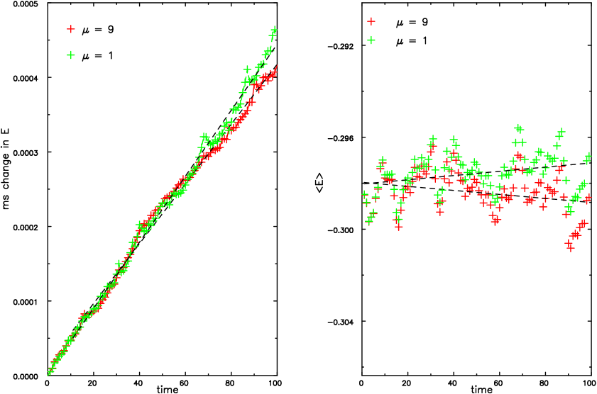
Figure 3: Results from a run of a Hernquist model with $N=2\times 10^{4}$ particles of each mass when forces are determined using the field method (SFP). The left panel shows the mean square change of energy of the particles, while the right panel shows the evolution of the mean specific energy (per unit mass) of the particles of each mass species.

4.2 Energy diffusion

The potential in a hypothetical simulation with infinitely many particles would be smooth and steady, assuming the model is a stable equilibrium, and the specific energy $E$ of each particle would be conserved. Therefore the time evolution of the rms changes in $E$ is one convenient measure of relaxation in a system with finite $N$.

Figure 3 presents a typical set of energy measurements from the particles in a simulation; values for heavy particles are drawn in red, while green is used for the light particles. The left panel gives the value of $\langle[E_{i}(t)-E_{i}(0)]^{2}\rangle$, the mean square change since the start in the measured specific energy of the particles. It can be seen that the value of this quantity rises roughly linearly with time, as HB90 found, indicating that the values are changing through a diffusive process. I fit a straight line to the last 90 values (i.e. ignoring the first 11, where the rise is often a little steeper), and henceforth report only this fitted slope as the mean square change of $E$ per dynamical time $t_{0}$, and its associated uncertainty.

The changes presented in Figure 3 are averages over all the particles. Naturally, the rms changes are larger for those particles whose orbit periods are shorter. As this trend is quite gradual in the inhomogeneous models and non-existent in the uniform models, the global averages I report in all cases are representative of those at intermediate radii where the bulk of the particles are located.

The total angular momentum, $L=|\;\kern-2.5pt\hbox{$\mit L$}\kern-6.25002pt\kern 0.50003pt\hbox{$\mit L$}\kern-6.25002pt\kern-0.24994pt\raise 0.43304pt\hbox{$\mit L$}|$, of each particle is also conserved in a smooth potential, and its changes afford another measure of relaxation. I have found that the mean-squared changes in $L$ also rise roughly linearly with time, but not quite as smoothly as the $E$ changes in the left panel of Figure 3. Furthermore, mass segregation is still less evident in the angular momentum changes. I therefore focus on the $E$ changes for the remainder of the paper.

4.3 Mass segregation

The right panel of Figure 3 gives the time evolution of the mean specific energy $\langle E_{i}(t)\rangle$ of the particles of the separate masses. The rapid variations have the same sign for each particle species because they arise from variations in $T+2W$, as discussed in §3, that are related to the virial fluctuations (Fig. 2). They result from evolving potential changes seeded by shot-noise driven fluctuations among the particles.

In addition to these fluctuations, the right panel of Figure 3 displays a slow divergence of the mean energies of the heavy and light particles, which represents the gradual exchange of energy that would in the long-run cause the heavy particles to settle to the centre and the lighter to populate the envelope of the model. The slopes of the straight lines fitted to these data should differ in magnitude by the ratio of the particle masses, since total energy conservation requires the energy lost by the heavy particles to be taken up by the light. In practice, this symmetry is imperfect because of the large measurement uncertainties. Henceforth, I report only the slopes, multiplied by $\mu$, and their statistical uncertainties.

In systems of gravitating particles, heavy particles lose energy to light particles through dynamical friction (Binney & Tremaine, 2008). Physically, a particle is braked by the attraction from its wake – i.e. the response of the surrounding sea of particles to its motion. In a system of equal mass particles, the frictional drag on each particle is balanced, on average, by the scattering accelerations (Hénon, 1973) and no secular changes occur. But differences between the braking and acceleration terms cause mass segregation when particle masses are unequal.

Were energy exchange between particles of the different mass species the only source of relaxation, the trends in the right panel of Figure 3 would not be strongly masked by short term oscillations. That short-term changes are larger than the gradual diverging trend is evidence that relaxation, measured in the left-hand panel, is being driven mostly by the collective oscillations of the model discussed above that are independent of particle masses.

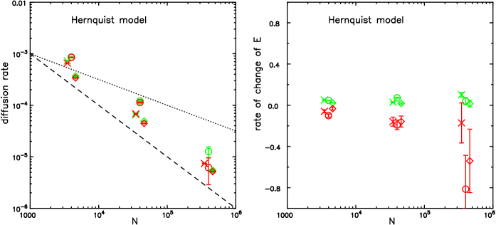
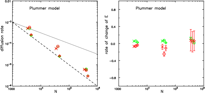
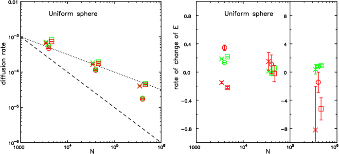
Figure 4: Summary of results from 27 simulations. The left column shows the $N$-dependence of the diffusion rate defined in eq. (5) and the right column shows $Nd\langle E_{i}(t)\rangle/dt$, with green points for the light particles and red for the nine times heavier particles. The top row is for the Hernquist model, the middle row for the Plummer model and the bottom row is for the uniform sphere. Crosses are from the tree code (BHT), circles from the spherical grid (S3D), diamonds from the field method (SFP) which was used for the Hernquist and Plummer models only, while squares are for a cubic Cartesian grid (C3D) which was used for the uniform sphere only. The error bars show $\pm\sigma$ uncertainties in the slopes, and the symbols from the different methods have been slightly shifted horizontally for clarity even though the same total numbers of particles, $N$, were used. Note that the vertical range is expanded by a factor of 10 for the points at the highest $N$ in the lower right panel.

4.4 Measures of relaxation rate

Figure 4 summarizes the relaxation measurements from all 27 simulations. The three rows show the three different mass models; within each panel there are three different numbers of particles, and for each case, the evolution was computed by three separate force determination methods. The measured rates from the heavy particles are shown in red, while those from the light particles are marked in green, and the uncertainties in the slopes are indicated by the error bars, that are often too short to be visible. The different force determination methods used are distinguished by the different symbol types as indicated in the figure caption, and offset horizontally from each other for clarity even though the particle numbers are the same. These conventions are the same in the left and right panels.

The left panels show the energy diffusion rate, defined as

$$\langle E_{i}(0)\rangle^{-2}\;{d\over dt}\langle[E_{i}(0)-E_{i}(t)]^{2}\rangle$$ (5)

in units of $t_{0}^{-1}$. The adopted values for $\langle E_{i}(0)\rangle$, which are $-0.3$, $-0.45$, $-0.9$ for the Hernquist, Plummer, and uniform sphere respectively, are the same for all nine simulations with each model. The straight dotted line has slope $-0.5$ while the slope of the dashed line is $-1$; these lines are not fits to the data and are for comparison only. The right panels show $Nd\langle E_{i}(t)\rangle/dt$, the factor $N$ for each sub-population is included for clarity – in reality, the slopes roughly decrease as $1/N$.

There are many conclusions to be drawn from these data.

First, the differences between the energy diffusion rates (left panels) for the heavy (red) and light (green) particles within one simulation are generally small. This is a further indication of the dominance of coherent potential variations, which cause deflections that are independent of particle mass, in driving this measure of relaxation.

Second, the energy diffusion rate declines roughly as $N^{-1/2}$ in the uniform sphere, whereas in the inhomogeneous models it declines more or less with the expected $N^{-1}$ dependence for collisional relaxation at fixed resolution (see §1). If two-body effects were dominant in all cases, the variation with $N$ should be the same in all three mass models.

Third, the rates of energy exchange shown in the right hand panels generally have opposite signs, and vary roughly as $N^{-1}$, since they are approximately constant when multiplied by $N$. The values from the highest $N$ experiments are quite uncertain, because the decreasing variation in the mean as $N$ rises is masked by short-term changes (see the right panel of Fig. 3) – i.e. the trends decrease into the noise. This is particularly problematic for the uniform sphere (bottom right panel), where the potential changes associated with pulsations of the model dominate over the energy exchange rate at the highest $N$, making an accurate measurement over the time interval simulated impossible.

Fourth, the different methods used to compute the gravitational field yield broadly similar behaviour in all three mass models, and the variation of the rates with $N$ in both the left and right panels is similar for each method in each of the different models.

Fifth, the energy diffusion rate (left panels) is consistently lower, but by a factor $<3$, for the SFP method (diamonds) than for the tree code (crosses) and the spherical grid (circles) in the Hernquist and Plummer models. This systematic difference is also present in the variations of $L$. Hernquist & Ostriker (1992) also reported a slightly lower energy diffusion rate when they used a field method, although it was unclear whether the more rapid diffusion in their tree code, for example, resulted mainly from the mild disequilbrium of their initial model caused by gravity softening. However, the mass segregation rate (right panels), which is a more direct consequence of two-body scattering, is no less for SFP than for the other methods.

Sixth, relaxation in the uniform sphere probably is completely dominated by the oscillatory modes excited by the shot noise in the particle distribution. The initial amplitudes of the modes should scale as $N^{-1/2}$, and the decline in relaxation rate with approximately this dependence in the uniform sphere is a direct indication of their dominance in this case. Collective modes are present in all models, but the different $N$-dependence in the inhomogeneous models is probably because modes are rapidly damped in those cases.

Seventh, short-range gravity softening appears to have little effect on the relaxation rate. There is no explicit softening in SFP, and the only smoothing on the spherical grid is linear interpolation in radius. Force softening is explicit in the tree code and implicit in the C3D grid, where forces are slightly sharper $\epsilon_{\rm eff}=0.036a$ while $\epsilon=0.05a$ for the BHT code for the uniform sphere. Yet the relaxation rates scarcely differ between the various codes. This emphasizes the dominance of distant encounters, enhanced by collective oscillations, in driving relaxation and that softening’s only value is to avoid large accelerations during close encounters between particles, which would require short time steps to integrate the motions accurately.

Once again, the quantities shown in Figure 4 are averages over all the particles, and these conclusions therefore apply to the particles in the bulk of the model. The small number of more tightly bound particles have the largest energy changes, but by factors of only a few, and therefore have little overall effect on the global average. Note also that their rate of energy change should be reckoned on the time-scale of their shorter orbit periods.

5 Discussion

5.1 Discrepancy with Weinberg & Katz (2007a, b)

The finding stated in point four above is in strong disagreement with that of Weinberg & Katz (2007a, b), who argued that the relaxation time-scale is orders of magnitude longer in field methods. It should be noted that their analysis addressed the more limited problem of resonant exchanges between particles and a perturbing bar potential, not the more general relaxation studied here. However, a discrepancy remains to be explained since Sellwood (2008), in a study that addressed their specific prediction, also found that field methods were not superior to grid methods.

Their calculation is highly technical but, in essence, they began by separating large- from small-scale noise and calculated separate contributions to the orbit deflections from both these “components” of the noise. Rather surprisingly, they found that deflections due to large-scale noise were much weaker than those from small-scale noise. They then argued that direct codes possess noise on both scales while field methods are affected only by large-scale noise, which led them to conclude that relaxation should be far slower in field methods. However, it is well-known that noise is present on all scales and, since every decade of impact parameter contributes equally to the Coulomb logarithm (Binney & Tremaine, 2008), there can be no clear distinction between large- and small-scale noise. This also implies that relaxation from large-scale noise should be comparable to that from small-scale noise.

5.2 More on collective effects

Vasiliev (2015) found good agreement between experimental relaxation rates and theoretical predictions from Fokker-Planck diffusion coefficients, suggesting that self-gravity of the collective modes does not boost the relaxation rate significantly. Furthermore, his predicted rate for the Plummer sphere is in good agreement with the value I find (Fig. 4, middle row, left panel).

However, such studies usually consider inhomogeneous models. The anomalous results presented here for the uniform sphere show that relaxation is greatly enhanced by collective modes in this unusual case where all orbits have the same period. Note that Rauch & Tremaine (1996) also found enhanced relaxation through collective effects in their study of a system of low-mass particles in near Keplerian motion about a central mass. In their case, it was important that particles with the same $L$ had the same period.

5.3 Mild dependence on method

The reason for the slightly lower diffusion rate in the field method (point five above) is unclear. Both the SFP and S3D methods employ an expansion in surface harmonics up to $l_{\rm max}=8$ to capture any angular variations, and the principal difference between them is radial resolution: the SFP method employs 11 radial functions ($0\leq n\leq 10$), while the S3D uses a grid of $\sim 100$ radial shells.

It therefore seemed that the marginally higher energy diffusion rate when the S3D grid was used was because that grid could support more oscillatory modes. However, increasing the number of radial functions used in the SFP method to 51, in order to enable the field method also to support more collective modes, led to little change in either measure of the relaxation rate, confounding this theory! Additional experiments with $l_{\rm max}=4$ and $l_{\rm max}=16$ caused very slight changes in the measured relaxation rates in the expected sense, but the systematic discrepancy between the two methods persisted.

While the puzzle remains, the negative outcome of these tests is further evidence of the unimportance of self-gravity for collective oscillations in inhomogeneous models.

6 Conclusions

The main result here confirms that previously found by Hernquist & Barnes (1990) and by Hernquist & Ostriker (1992) that the rate of relaxation in $N$-body simulations that aspire to be collisionless is very largely independent of the method used to compute the gravitational field. This is especially true when the relaxation rate is assayed as the rate of energy exchange between particles of different masses – see the right hand panels of Fig. 4. This result is physically reasonable, since relaxation is dominated by distant encounters and any method that correctly yields the field from distant particles must faithfully include their stochastic contributions.

The rate of relaxation arises from at least two distinguishable sources: a slow diffusion of the integrals caused by coherent potential oscillations of the system that are largely independent of particle mass, and mass segregation that is more directly caused by two-body encounters. The good agreement (§5.2) between Fokker-Planck diffusion and $N$-body experiment in the inhomogeneous models indicates that self-gravity of the collective modes adds little to the relaxation rate. The rate of energy exchange between particles of differing masses becomes more difficult to measure as $N$ rises because mean energies scatter with potential variations that scale as $N^{-1/2}$, while the trends in the mean energies of the different mass species diverge as $N^{-1}$.

The different $N$-dependence in the uniform sphere (bottom left panel of Fig. 4) is clear evidence that collective modes do dominate the relaxation in this special case. This model differs from the other two by having a harmonic potential throughout in which the orbit frequencies of all particles are the same; this difference permits undamped collective oscillations, whereas collective modes are damped in the other cases.

The slightly lower energy diffusion rates that result from use of the field method (diamonds in top left and middle left panels of Fig. 4) is bought at a high price. The leading term in the basis used for both cases was a perfect match to the equilibrium model, and the same basis would be less suited were the density to evolve, or were it used for any other model, requiring more terms to yield the correct total potential. Thus field methods lack the versatility to follow arbitrary changes to the distribution of mass within a model unless the expansion is taken to higher order, and their slightly better relaxation rate can be achieved in any of the more general methods simply by employing a few times more particles. A real advantage of field methods, featured by Weinberg & Katz (2007a, b), is that they offer an elegant comparison of simulations with perturbation theory when computing first order changes to an equilibrium model that could be unstable or externally perturbed.

The energy diffusion time-scale, the inverse of the rate defined in eq. (5) and plotted in Fig. 4, is $\ga 10^{5}$ dynamical times (i.e. $10^{12}$ yr for the suggested scaling) for only $N=4\times 10^{5}$ particles in the inhomogeneous models (it is shorter for the exotic case of the uniform sphere). By this measure, relaxation times in simulations of inhomogeneous 3D models using any valid code are already significantly longer than the ages of the galaxies being simulated, and relaxation considerations alone do not require much larger numbers of particles.

References

- (1)
- Barnes & Hut (1986) Barnes, J. & Hut, P. 1986, Nature, 324, 446
- Binney & Tremaine (2008) Binney, J. & Tremaine, S. 2008, Galactic Dynamics (2nd ed.; Princeton: Princeton University Press)
- Chandrasekhar (1941) Chandrasekhar, S. 1941, ApJ, 94, 511
- Clutton-Brock (1972) Clutton-Brock, M. 1972, Ap. Sp. Sci., 17, 292
- Debattista & Sellwood (2000) Debattista, V. P. & Sellwood, J. A. 2000, ApJ, 543, 704
- Hénon (1973) Hénon, M. 1973, in Dynamical Structure and Evolution of Stellar Systems, ed. L. Martinet & M. Mayor (Sauverny: Geneva Observatory) p. 182
- Hernquist (1990) Hernquist, L. 1990, ApJ, 356, 359
- Hernquist & Barnes (1990) Hernquist, L. & Barnes, J. E. 1990, ApJ, 349, 562
- Hernquist & Ostriker (1992) Hernquist, L. & Ostriker, J. P. 1992, ApJ, 386, 375
- Hockney & Eastwood (1981) Hockney, R. W. & Eastwood, J. W. 1981, Computer Simulation Using Particles , New York:McGraw Hill
- Holley-Bockelmann, Weinberg & Katz (2005) Holley-Bockelmann, K., Weinberg, M. & Katz, N. 2005, MNRAS, 363, 991
- James (1977) James, R. A. 1977, J. Comp. Phys., 25, 71
- McGlynn (1984) McGlynn, T. A. 1984, ApJ, 281, 13
- Merritt (2013) Merritt, D. 2013, Dynamics and Evolution of Galactic Nuclei (Princeton: Princeton University Press)
- Monaghan (1992) Monaghan, J. J. 1992, ARAA, 30, 543
- Plummer (1911) Plummer, H. C. 1911, MNRAS, 71, 460
- Polyachenko & Shukhman (1979) Polyachenko, V. L. & Shukhman, I. G. 1979, Astron. Zh. 56, 724; English translation: 1981, Sov. Astron., 25, 533
- Rauch & Tremaine (1996) Rauch, K. P. & Tremaine, S. 1996, New. Astron., 1, 149
- Rostoker & Rosenbluth (1960) Rostoker, N. & Rosenbluth, M. N. 1960, Phys. Fluids, 3, 1
- Sellwood (2003) Sellwood, J. A. 2003, ApJ, 587, 638
- Sellwood (2008) Sellwood, J. A. 2008, ApJ, 679, 379
- Sellwood (2013) Sellwood, J. A. 2013, ApJL, 769, L24
- Sellwood (2014) Sellwood, J. A. 2014, arXiv:1406.6606 (on-line manual: http://www.physics.rutgers.edu/sellwood/manual.pdf)
- Sellwood & Merritt (1994) Sellwood, J. A. & Merritt, D. 1994, ApJ, 425, 530
- Spitzer (1987) Spitzer, L. 1987, Dynamical Evolution of Globular Clusters (Princeton: Princeton University Press)
- Springel (2005) Springel, V. 2005, MNRAS, 364, 1105
- Vasiliev (2015) Vasiliev, E. 2015, MNRAS, 446, 3150
- Weinberg (1998) Weinberg, M. D. 1998, MNRAS, 297, 101
- Weinberg (1999) Weinberg, M. D. 1999, AJ, 117, 629
- Weinberg & Katz (2007a) Weinberg, M. D. & Katz, N. 2007a, MNRAS, 375, 425
- Weinberg & Katz (2007b) Weinberg, M. D. & Katz, N. 2007b, MNRAS, 375, 460