Projective classification of jets of surfaces in $3$-space

Abstract.

We present a local classification of smooth surfaces in $\mathbb{P}^{3}$ via projective transformations in accordance with singularity types of central projections with codimension $\leq 4$. We also discuss relations between our classification of Monge forms and bifurcations of parabolic curves and flecnodal curves.

1. Introduction

1.1. Normal forms

In projective differential geometry, local properties of a surface in $3$-space was intensively investigated by Darboux and others from the end of the 19th century to the early 20th century, while some new interests and ideas have recently been brought from singularity theory, generic differential geometry and applied mathematics such as computer-vison [1, 2, 4, 13, 14, 17, 18, 21, 25, 26]; for example, geometric features of a multi-parameter family of surfaces in $3$-space are of particular interest in application [26]. In the present paper, we deal with a classification of jets of surfaces in $\mathbb{P}^{3}$ via projective transformations, which gives a new insight of the classical subject from a singularity theoretic approach. We mainly work over $\mathbb{R}$. Throughout this paper, we identify $\mathbb{R}^{3}$ with an open chart of the projective space, $\{[x:y:z:1]\}\subset\mathbb{P}^{3}$, and consider germs of surfaces in $\mathbb{R}^{3}$ at the origin given by Monge forms $z=f(x,y)$ with $f(0)=0$ and $df(0)=0$. We say that two germs or jets of surfaces are projectively equivalent if there is a projective transformation on $\mathbb{P}^{3}$ sending one to the other. A classically well-known fact is that at a general hyperbolic point of a surface, the jet of the Monge form is projectively equivalent to

$$xy+x^{3}+y^{3}+\alpha x^{4}+\beta y^{4}+\cdots$$

where moduli parameters $\alpha,\beta$ are primary projective differential invariants (those should be compared with the Gaussian/mean curvatures in the Euclidean case and the Pick invariant in the equi-affine case, cf. [16, 24, 28]). Our aim is to present this kind of expression for degenerate Monge forms. Most interesting is the parabolic case.

Projective transformations preserving the origin and the $xy$-plane form a $10$-dimensional subgroup of $PGL(4)$, and it acts on the space of jets of Monge forms. We then give an invariant stratification of the jet space of Monge forms in accordance with singularity types of central projections, and describe the normal form of each stratum up to codimension $4$. This is a natural extension of results of Platonova [17] and Landis [14] (see also [1, 2, 12]) on the classification of jets of Monge forms for a generic surface, which corresponds to the case of codimension $\leq 2$ in our list. Our main theorem is stated as follows:

Theorem 1.1.

Let $M$ be a closed surface and $U$ an open neighborhood of the origin in $\mathbb{R}^{2}$ (parameter space). There is a residual subset $\mathcal{O}$ of the space of $2$-parameter families of smooth embeddings $\phi:M\times U\to\mathbb{P}^{3}$ equipped with $C^{\infty}$-topology so that each $\phi\in\mathcal{O}$ satisfies that for arbitrary point $(x_{0},u)\in M\times U$ the $p$-jet of Monge form of the surface $M_{u}(=\phi(M\times u))$ at $x_{0}$ is projectively equivalent to one of the normal forms at the origin given in Tables 1, 2, 3 with codimension $s\;(\leq 4)$.

In Tables, $\alpha,\beta,\cdots$ are moduli parameters and $\phi_{k}$ denotes arbitrary homogeneous polynomials of degree $k$. In our stratification, each stratum is determined by its projection type (i.e. singularity type of projection along the asymptotic line), that is explained in the next §1.2 and §2.2. This characterization is quite relevant – e.g. classes $\Pi^{p}_{{\rm I},k}$ can not be distinguished by using types of height functions, the parabolic curves and asymptotic curves, but can be so by the difference of singularity types of projection from a special isolated viewpoint. The same approach to the classification of surfaces in $\mathbb{P}^{4}$ is considered in [11].

$$\begin{array}[]{l | l | c c | l }\mbox{class}&\mbox{normal form}&\mbox{p}&\mbox{s}&\mbox{proj. }\\ \hline\cr\hline\cr\Pi^{p}_{{\rm I},1}&y^{2}+x^{3}+xy^{3}+\alpha x^{4}&4&1&{\rm I}_{2}\,({\rm I}_{3})\\ \Pi^{p}_{{\rm I},2}&y^{2}+x^{3}\pm xy^{4}+\alpha x^{4}+\beta y^{5}+x^{2}\phi_{3}&5&2&{\rm I}_{2}\,({\rm I}_{4})\\ \Pi^{p}_{c,1}&y^{2}+x^{2}y+\alpha x^{4}\;\;\;(\alpha\not=0,\frac{1}{4})&4&2&{\rm III}_{2}\,({\rm III}_{3})\\ \hline\cr\Pi^{p}_{c,2}&y^{2}+x^{2}y+\frac{1}{4}x^{4}+\alpha x^{5}+y\phi_{4}\;(\alpha\not=0)&5&3&{\rm III}_{2}\\ \Pi^{p}_{c,4}&y^{2}+x^{2}y+x^{5}+y\phi_{4}&5&3&{\rm IV}_{1}\\ \Pi^{p}_{{\rm I},3}&y^{2}+x^{3}+xy^{5}+\alpha x^{4}+\phi&6&3&{\rm I}_{2}\,({\rm I}_{5})\\ \Pi^{p}_{v,1}&y^{2}\pm x^{4}+\alpha x^{3}y+\beta x^{2}y^{2}\;\;(\beta\not=\pm\frac{3}{8}\alpha^{2})&4&3&{\rm V}_{1}\,({\rm VI})\\ \Pi^{p}_{c,3}&y^{2}+x^{2}y+\frac{1}{4}x^{4}+y\phi_{4}&5&4&{\rm III}_{3}\,({\rm III}_{4})\\ \Pi^{p}_{c,5}&y^{2}+x^{2}y\pm x^{6}+y(\phi_{4}+\phi_{5})&6&4&{\rm IV}_{2}\\ \Pi^{p}_{{\rm I},4}&y^{2}+x^{3}+\alpha x^{4}+\phi&6&4&{\rm I}_{2}\,({\rm I}_{6})\\ \Pi^{p}_{v,2}&y^{2}\pm x^{4}+\alpha x^{3}y\pm\frac{3}{8}\alpha^{2}x^{2}y^{2}&4&4&{\rm V}_{1}\,({\rm VI}_{1})\\ \Pi^{p}_{v,3}&y^{2}+x^{5}+y(\phi_{3}+\phi_{4})&5&4&{\rm V}_{2}\,({\rm VI}_{2})\\ \end{array}$$

Table 1. Parabolic case. In normal forms, $\phi_{k}$ denotes homogeneous polynomials of degree $k$ (that is also in Tables 2, 3). For $\Pi^{p}_{{\rm I},k}\;(k=3,4)$, we put $\phi=\beta y^{5}+\gamma y^{6}+x^{2}(\phi_{3}+\phi_{4})$ for short. Double-sign $\pm$ corresponds in same order for each of $\Pi^{p}_{v,1}$ or $\Pi^{p}_{v,2}$. For $\Pi^{p}_{c,1}$, if $\alpha=1$, the normal form of $4$-jet should be $y^{2}+x^{2}y+x^{4}+\beta x^{3}y$.

$$\begin{array}[]{l | l | c c | l }\mbox{class}&\mbox{normal form}&\mbox{p}&\mbox{s}&\mbox{proj. }\\ \hline\cr\hline\cr\Pi^{h}_{3,3}&xy+x^{3}+y^{3}+\alpha x^{4}+\beta y^{4}&4&0&{\rm II}_{3}/{\rm II}_{3}\\ \Pi^{h}_{3,4}&xy+x^{3}+y^{4}+\alpha xy^{3}&4&1&{\rm II}_{3}/{\rm II}_{4}\\ \Pi^{h}_{3,5}&xy+x^{3}+y^{5}+\alpha xy^{3}+x\phi_{4}&5&2&{\rm II}_{3}/{\rm II}_{5}\\ \Pi^{h}_{4,4}&xy+x^{4}\pm y^{4}+\alpha xy^{3}+\beta x^{3}y&4&2&{\rm II}_{4}/{\rm II}_{4}\\ \hline\cr\Pi^{h}_{3,6}&xy+x^{3}+y^{6}+\alpha xy^{3}+x(\phi_{4}+\phi_{5})&6&3&{\rm II}_{3}/{\rm II}_{6}\\ \Pi^{h}_{4,5}&xy+x^{4}+y^{5}+\alpha xy^{3}+\beta x^{3}y+x\phi_{4}&5&3&{\rm II}_{4}/{\rm II}_{5}\\ \Pi^{h}_{3,7}&xy+x^{3}+y^{7}+\alpha xy^{3}+x(\phi_{4}+\phi_{5}+\phi_{6})&7&4&{\rm II}_{3}/{\rm II}_{7}\\ \Pi^{h}_{4,6}&xy+x^{4}\pm y^{6}+\alpha xy^{3}+\beta x^{3}y+x(\phi_{4}+\phi_{5})&6&4&{\rm II}_{4}/{\rm II}_{6}\\ \Pi^{h}_{5,5}&xy+x^{5}+y^{5}+\alpha xy^{3}+\beta x^{3}y+xy\phi_{3}&5&4&{\rm II}_{5}/{\rm II}_{5}\end{array}$$

Table 2. Hyperbolic case. There are two projection types with respect to distinct asymptotic lines. Here ${\rm II}_{3}$ is of ordinary cusp.

$$\begin{array}[]{l | l | c c | l }\mbox{class}&\mbox{normal form}&\mbox{p}&\mbox{s}&\mbox{proj.}\\ \hline\cr\hline\cr\Pi^{e}&x^{2}+y^{2}&2&0&\mbox{\footnotesize\rm fold}\\ \hline\cr\Pi^{f}_{1}&xy^{2}\pm x^{3}+\alpha x^{3}y+\beta y^{4}&4&3&{{\rm I}_{2}^{\pm}}^{\dagger}\\ \Pi^{f}_{2}&xy^{2}+x^{4}\pm y^{4}+\alpha x^{3}y&4&4&{{\rm I}_{2}^{-}}^{\dagger}\\ \end{array}$$

Table 3. Umbilical case (elliptic and flat umbilic cases). For $\Pi^{e}_{k,j}\;(k,j\geq 4)$, we put $\phi=\beta x^{3}y+\gamma xy^{3}$ for short. $\dagger$: The projection type of $\Pi^{f}_{k}\;(k=1,2)$ are generically of type ${\rm I}_{2}$, see §2.3 for the detail.

Remark 1.2.

In the case over $\mathbb{C}$, the elliptic case and the sign difference in Tables are omitted. Theorem 1.1 can be restated in the algebro-geometric context by mean of a Beltini-type theorem for the linear system of projective surfaces of degree greater than $p$.

Remark 1.3.

In the normal forms listed in Tables, continuous moduli parameters $\alpha,\beta,\cdots$ and higher coefficients must be projective differential invariants in the sense of Sophus Lie; in fact, there is a similarity between our arguments and those in a modern theory of differential invariants due to Olver [16]. Besides, those leading parameters may have some particular geometric meanings. For instance, at a cusp of Gauss (that is a point of type $\Pi^{p}_{c,1}$ on the surface), the coefficient $\alpha$ of $x^{4}$ in the normal form coincides with the Uribe-Vargas cross-ratio invariant defined in [25]. Further, we will see that the coefficient of $x^{5}$ in the same Monge form corresponds to the position of a special viewpoint lying on the asymptotic line (§2.2). Also we discuss in the final section §4 a partial connection between our Monge forms and a topological classification of differential equations (BDE) defining nets of asymptotic curves (§1.3); indeed $\alpha,\beta,\cdots$ are related to initial moduli parameters of the BDE.

1.2. Singularities of projections

In singularity theory, map-germs are classified up to diffeomorphism-germs of source and target, that is called the $\mathcal{A}$-equivalence of map-germs; we denote by $f\sim_{\mathcal{A}}g$ for $\mathcal{A}$-equivalent map-germs $f$ and $g$. Given a surface $M\subset\mathbb{P}^{3}$, the restriction of linear projection $\pi_{p}:\mathbb{P}^{3}-p\to\mathbb{P}^{2}$ from arbitrary viewpoint $p$ not lying on $M$ is called the central projection; for each point $x\in M$, it locally presents a map-germ $\pi_{p}|_{M}:\mathbb{R}^{2},0\to\mathbb{R}^{2},0$ by taking local coordinates centered at $x$ and $\pi_{p}(x)$ of source and target, respectively. Obviously, if two germs of surfaces are projectively equivalent, then they admit the same $\mathcal{A}$-types of projections from arbitrary viewpoints. As a generalization of Arnold-Platonova’s result [18], Kabata studied in [13] central projections of generic families of surfaces in the context of $\mathcal{A}$-classification theory of plane-to-plane germs [12, 19, 20]. In particular, he showed that all $\mathcal{A}$-types of $\mathcal{A}$-codimension $\leq 6$ appear in central projections of generic $2$-parameter families of surfaces. We then use part of Kabata’s result and classify jets of degenerate Monge forms up to projective transformations. In particular, Platonova’s degenerate classes $\Pi_{*}^{(k)}\;(k\geq 1)$ in [17, Table 2] break into much finer classes in jet spaces of higher order.

($\mathcal{A}$-classification) Typical singularities are of fold and cusp types, whose normal forms are given by $(y,x^{2})$ and $(y,xy+x^{3})$, respectively. More complicated $\mathcal{A}$-types of plane-to-plane map-germs are classified by Rieger [19, 20]. We follow his notations; $\mathcal{A}$-types with codimension $\leq 6$ are named by $1,2,\cdots,19$ as in [19, Table 1 (p.352)]. Some $\mathcal{A}$-types are combined into a single topological-$\mathcal{A}$-type, that was studied in detail in [20]; they are characterized by some specified $p$-jets listed in Table 4 below, and called equisingularity types ${\rm I}_{k},\cdots,{\rm VI}$ (see [13]). For our convenience, provisionally we add two types of $4$-jets with codimension greater than $6$, which are adjacent to ${\rm VI}$ ($c\not=0$):

$${\rm VI}_{1}:\;(y,x^{4}+dxy^{3}),\quad{\rm VI}_{2}:(y,cx^{2}y^{2}+dxy^{3}).$$

$$\begin{array}[]{c | c |l | c | c }\mbox{type}&\mbox{$\mathcal{A}$-type}&\mbox{normal forms of $p$-jets}&p&\mbox{codim.}\\ \hline\cr{\rm I}_{k}&4_{k}^{\pm}&(y,x^{3}\pm xy^{k})&k+1&k+1\\ {\rm II}_{k}&5-10&(y,xy+x^{k})&k&k-1\\ {\rm III}_{k}&11_{2k+1}&(y,x^{2}y+x^{4}+x^{2k+1})&2k+1&k+2\\ {\rm IV}_{1}&12,13,14&(y,x^{2}y+x^{5})&5&5\\ {\rm IV}_{2}&15&(y,x^{2}y+x^{6})&6&6\\ {\rm V}_{1}&16,17&(y,xy^{2}+x^{4})&4&5\\ {\rm V}_{2}&18&(y,xy^{2}+dx^{3}y)&4&6\\ {\rm VI}&19&(y,x^{4}+cx^{2}y^{2}+dxy^{3})&4&6\end{array}$$

Table 4. Equisingularity types of plane-to-plane germs with $\mathcal{A}$-codimension $\leq 6$ [20]

(Projection type) The projection type in Tables means the $\mathcal{A}$-type of the central projection from arbitrary viewpoint lying on the asymptotic line. Here the entire Monge form is assumed to have appropriately generic higher terms of order $>p$ added to the prescribed normal forms of $p$-jet in Tables.

For instance, look at the class $\Pi^{p}_{c,1}$; the stratum has codimension $2$ in the jet space, thus the class appears at some isolated point on a generic surface, that is classically called an (ordinary) cusp of Gauss point. In Table 1 the corresponding projection type is written as “${\rm III}_{2}\,({\rm III}_{3})$”. That means that the central projection from almost all viewpoints lying on the asymptotic line has the Gulls singularity ${\rm III}_{2}$, while the projection from some exceptional isolated viewpoint is of type ${\rm III}_{3}$ worse than Gulls type. If $\alpha=0$, we have the degenerate class $\Pi^{p}_{c,4}$; it has codimension $3$, so it appears generically in $1$-parameter family of surfaces with the projection type ${\rm IV}_{1}$. In case that $\alpha=\frac{1}{4}$, there are two degenerate classes $\Pi^{p}_{c,2}$ and $\Pi^{p}_{c,3}$ according to whether the term $x^{5}$ in the $5$-jet remains or not. The latter type appears generically in a $2$-parameter family of surfaces, and the projection from any viewpoints on the asymptotic line is of type ${\rm III}_{3}$ or worse. See §2.2 for the detail.

1.3. Net of asymptotic curves

At each hyperbolic point of a surface in $\mathbb{P}^{3}$, there are exactly two asymptotic lines (lines tangent to the surface with more than $2$-point contact); they are invariants under projective transformations. The integral curves, called asymptotic curves, form a pair of foliations on the hyperbolic domain, which is classically named by the net of asymptotic curves. The parabolic curve is the locus of singular points of asymptotic curves, and in fact it is the locus of points on the surface whose Monge form is of type $\Pi^{p}_{{\rm I},1}$ or more degenerate ones. The flecnodal curve is the locus of inflection points of asymptotic curves; it is actually the closure of the locus of class $\Pi^{h}_{3,4}$. The parabolic and flecnodal curves meet each other tangentially at a cusp of Gauss, i.e. a point of class $\Pi^{p}_{c,k}\;(k\geq 1)$.

The net of asymptotic curves is defined by a binary differential equation (BDE). In a general setting, Davydov [9, 10] and Bruce-Tari [4, 5, 6, 22, 23] has presented the topological classification of (families of) BDE. We then compare our classification of parabolic Monge forms with degenerate parabolic points arising in the general classification of BDE (Propositions 4.1, 4.3, 4.4). In particular, we will see that the flat umbilic class $\Pi^{f}_{2}$ corresponds to a type of generic $3$-parameter family of BDE studied in Oliver [15]. Furthermore, we also compare our classification of hyperbolic Monge forms with bifurcations of flecnodal curves. In part of his dissertation [26] Uribe-Vargas presented a complete list of generic $1$-parameter bifurcations of flecnodal curves via a geometric approach using the dual surfaces. We give a precise characterization of moduli parameters in our corresponding Monge form for each type of Uribe-Vargas’ classification.

Acknowledgement

The authors would like to thank Takashi Nishimira and Farid Tari for organizing the JSPS-CAPES international cooperation project in 2014-2015. In fact, the second and third authors are supported by the project for their stays in ICMC-USP and Hokkaido University, respectively. The authors also thank Ricardo Uribe-Vargas for letting us know of his paper [26] and for his valuable comments. They are partly supported by JSPS grants no.24340007 and 15K13452.

2. Jets of Monge forms

2.1. Central projection

Assume that $\mathbb{R}^{4}$ is equipped with the standard inner product. Let $p=[\mbox{\boldmath$p$}]\in\mathbb{P}^{3}$, called a viewpoint, and let $W_{p}\subset\mathbb{R}^{4}$ denote the orthogonal complement to the vector $\mbox{\boldmath$p$}\in\mathbb{R}^{4}$. The central projection $\pi_{p}$ is the map from $\mathbb{P}^{3}-\{p\}$ to the projectivization $\mathbb{P}(W_{p})$ given by

$$\pi_{p}([\mbox{\boldmath$u$}])=\left[\mbox{\boldmath$u$}-\frac{(\mbox{\boldmath$u$}\cdot\mbox{\boldmath$p$})\mbox{\boldmath$p$}}{||\mbox{\boldmath$p$}||^{2}}\right]\in\mathbb{P}(W_{p})\subset\mathbb{P}^{3}.$$

Restrict $\pi_{p}$ to the open set $\mathbb{R}^{3}\subset\mathbb{P}^{3}$. For $\mbox{\boldmath$p$}=(a,b,c,1)\in\mathbb{R}^{4}$, set

$$A=\left(\begin{array}[]{rrrr}1&0&0&-a\\ 0&1&0&-b\\ 0&0&1&-c\\ -a&-b&-c&-1\end{array}\right)$$

and $\Phi_{A}:\mathbb{P}^{3}\to\mathbb{P}^{3}$ the projective transformation defined by $A$. Obviously, $\Phi_{A}(p)=0\in\mathbb{R}^{3}$ and $\Phi_{A}(W_{p})=\mathbb{P}^{2}$. We identify $\pi_{p}$ with

$$\Phi_{A}\circ\pi_{p}:\mathbb{R}^{3}-\{p\}\to\mathbb{P}^{2},\quad(x,y,z)\mapsto[x-a:y-b:z-c].$$

If the viewpoint is at infinity, i.e. $\mbox{\boldmath$p$}=(p,0)$ with $p=(a,b,c)\in\mathbb{R}^{3}$, then the projection is given by for $\mbox{\boldmath$u$}=(u,1)\in\mathbb{R}^{4}$

$$\pi_{p}([\mbox{\boldmath$u$}])=\left[\mbox{\boldmath$u$}-\frac{(\mbox{\boldmath$u$}\cdot\mbox{\boldmath$p$})\mbox{\boldmath$p$}}{||\mbox{\boldmath$p$}||^{2}}\right]=\left[u-\frac{(u\cdot p)p}{||p||^{2}}:1\right]\;\;\in\mathbb{P}(W_{p}).$$

Hence it induces the orthogonal projection (or parallel projection) in $\mathbb{R}^{3}$ along the line generated by the vector $p$; if $a\not=0$ and $v=b/a$, $w=c/a$, then we have by a linear transform on target $\mathbb{R}^{2}$

$$\pi_{p}:\mathbb{R}^{3}\to\mathbb{R}^{2},\quad\pi_{p}(x,y,z)=(y-vx,z-wx).$$

Let $M$ be a surface in $\mathbb{R}^{3}\;(\subset\mathbb{P}^{3})$ around the origin with the Monge form

$$z=f(x,y)=\sum_{i+j\geq 2}c_{ij}x^{i}y^{j}.$$

Take a viewpoint $p=(a,b,c)$ with $a\not=0$, and then the central projection from $p$ is locally written by

$$\varphi_{p,f}=\pi_{p}|_{M}:M\to\mathbb{R}^{2},\;\;\;(x,y)\mapsto\left(\frac{y-b}{x-a},\frac{f(x,y)-c}{x-a}\right)=(X,Y)$$

using local coordinates $(x,y)$ of $M$ and $[1:X:Y]$ of $\mathbb{P}^{2}$. If $p$ is chosen to be at infinity in $\mathbb{P}^{3}$, then

$$\varphi_{p,f}(x,y)=\left(y-vx,f(x,y)-wx\right).$$

Given a surface $M$ and a point $x\in M$, we are interested in the singularity types (as plane-to-plane map-germs) of central projections $\varphi_{p,f}:M,x\to\mathbb{R}^{2},0$ from arbitrary viewpoint $p\in\mathbb{P}^{3}-M$. We say two germs $\eta_{1},\eta_{2}:\mathbb{R}^{2},0\to\mathbb{R}^{2},0$ are $\mathcal{A}$-equivalent if there are diffeomorphism-germs $\sigma,\tau$ of source and target $\mathbb{R}^{2}$ at the origins such that $\eta_{2}=\tau\circ\eta_{1}\circ\sigma^{-1}$.

2.2. Criteria

Now, assume that the $x$-axis is an asymptotic line of $M$ at the origin and $p$ lies on it, i.e. $b=c=0$. Then, taking new coordinate $\bar{x}=x$ and $\bar{y}=y(x-a)^{-1}$, the projection is of the form

$$\varphi_{p,f}=\left(\bar{y},\frac{f(\bar{x},\bar{y}(\bar{x}-a))}{\bar{x}-a}\right).$$

According to Rieger’s classification [19] and useful criteria in [13] for $\mathcal{A}$-types of plane-to-plane germs, one can determine local types of singularities of $\varphi_{p,f}$. In fact, for each $\mathcal{A}$-type in Rieger’s list, Kabata explicitly described in [13] the necessary and sufficient condition on coefficients $c_{ij}$ so that the germ of $\varphi_{p,f}$ at the origin is $\mathcal{A}$-equivalent to the type. Elliptic case and umbilical case are easy, so we omit them. For the hyperbolic and parabolic cases, we may assume that $j^{2}f=xy$ and $j^{2}f=y^{2}$, respectively, by some linear transformation. In Tables 5 and 6, the middle column stands for Kabata’s closed condition on $c_{ij}$ and the right is the corresponding projection type, i.e. the $\mathcal{A}$-type of $\varphi_{p,f}$. The condition defines an invariant stratum named by class $\Pi^{*}_{*,*}$ (left). Notice that some open condition on $c_{ij}$ is implicitly imposed for each class in the list, e.g., in Table 5, we understand that $c_{40}\not=0$ for $\Pi^{h}_{3,4}$ to distinguish the type from others.

$$\begin{array}[]{l l l}&\mbox{\footnotesize cond.}&\mbox{\footnotesize type }\\ \hline\cr\Pi^{h}_{3,4}&c_{30}=0&{\rm II}_{4}\\ \Pi^{h}_{3,5}&c_{30}=c_{40}=0&{\rm II}_{5}\\ \Pi^{h}_{3,6}&c_{30}=c_{40}=c_{50}=0&{\rm II}_{6}\\ \Pi^{h}_{3,7}&c_{30}=c_{40}=c_{50}=c_{60}=0&{\rm II}_{7}\\ \end{array}$$

Table 5. Criteria of ($\mathcal{A}$-) equiangularity types for projections at a hyperbolic point [13]. It is assumed that $c_{11}\not=0$ and $c_{20}=c_{02}=0$. If $c_{30},c_{03}\not=0$, then it is a general hyperbolic point ($\Pi^{h}_{3,3}$), where the projection is of type cusp. The flecnodal curve consists of points of type $\Pi^{h}_{3,k}\;(k\geq 4)$, and its self-intersection points are of type $\Pi^{h}_{4,4}$ etc.

$$\begin{array}[]{l l l}&\mbox{\footnotesize cond.}&\mbox{\footnotesize type}\\ \hline\cr\Pi^{p}_{{\rm I},1}&c_{20}=0&{\rm I}_{2}\,({\rm I}_{3})\\ \Pi^{p}_{{\rm I},2}&c_{20}=P=0&{\rm I}_{2}\,({\rm I}_{4})\\ \Pi^{p}_{{\rm I},3}&c_{20}=P=Q=0&{\rm I}_{2}\,({\rm I}_{5})\\ \Pi^{p}_{{\rm I},4}&c_{20}=P=Q=R=0&{\rm I}_{2}\,({\rm I}_{6})\\ \hline\cr\Pi^{p}_{c,1}&c_{20}=c_{30}=0&{\rm III}_{2}\,({\rm III}_{3})\\ \Pi^{p}_{c,2}&c_{20}=c_{30}=B=0&{\rm III}_{2}\\ \Pi^{p}_{c,3}&c_{20}=c_{30}=A=B=0&{\rm III}_{3}\,({\rm III}_{4})\\ \Pi^{p}_{c,4}&c_{20}=c_{30}=c_{40}=0&{\rm IV}_{1}\\ \Pi^{p}_{c,5}&c_{20}=c_{30}=c_{40}=c_{50}=0&{\rm IV}_{2}\\ \hline\cr\Pi^{p}_{v,1}&c_{20}=c_{30}=c_{21}=0&{\rm V}_{1}\,({\rm VI})\\ \Pi^{p}_{v,2}&c_{20}=c_{30}=c_{21}=S=0&{\rm V}_{1}\,({\rm VI}_{1})\\ \Pi^{p}_{v,3}&c_{20}=c_{30}=c_{21}=c_{40}=0&{\rm V}_{2}\,({\rm VI}_{2})\\ \end{array}$$

Table 6. Criteria of ($\mathcal{A}$-) equiangularity types for projections at a parabolic point [13]. It is assumed that $c_{11}=0$ and $c_{02}\not=0$, and $A,B,P,\cdots,S$ are some polynomials in $c_{ij}$. A point of type $\Pi^{p}_{c,k}\;(k\geq 1)$ is an ordinary/degnerate cusp of Gauss point.

In Table 6 of the parabolic case, $A,B,P,\cdots$ are polynomials in $c_{ij}$ given as follows. They are defined by Kabata’s criteria for the appearance of singularity types ${\rm I}_{k}$, ${\rm III}_{k}$ and ${\rm VI}$ in central projections from special isolated viewpoints. We explain it below (see also [13]); it is always assumed that $c_{11}=0$, $c_{02}\not=0$ and $p=(a,0,0)$ with $a\not=0$ (possibly $a=\infty$).

(${\rm I}_{k}$)    $j^{3}\varphi_{p,f}\sim_{\mathcal{A}^{3}}(y,x^{3}+\delta xy^{2})$ for some $\delta$ if and only if $c_{20}=0$ and $c_{30}\not=0$.
Here $\delta$ is written by a non-zero scalar multiple of $Ca+D$ with

$$C=c_{21}^{2}-3c_{30}c_{12},\quad D=3c_{02}c_{30}\;\;(\not=0)$$

(if $p$ is at the infinity, that is, $\varphi_{p,f}$ is the parallel projection, $\delta=C/c_{30}^{2}$). The type ${\rm I}_{2}$ (lips/beaks) is just the case of $\delta\not=0$. Therefore, the projection is of type ${\rm I}_{2}$ from almost all viewpoints lying on the asymptotic line ($x$-axis), i.e. $Ca+D\not=0$, while there is a unique viewpoint $p=(-D/C,0,0)$ (or the infinity if $C=0$) so that the projection is of type ${\rm I}_{3}$ or worse. Let $p$ be the special viewpoint. Then the degenerate projection is written by $\varphi_{p,f}=(y,x^{3}+\sum_{i+j\geq 4}a_{ij}x^{i}y^{j})$ in some local coordinates; we put

$$\textstyle P=a_{13},\;\;Q=a_{14}-\frac{1}{3}a_{22}^{2},\;\;R=a_{15}-\frac{2}{3}a_{23}a_{22}+\frac{1}{3}a_{31}a_{22}^{2}.$$

It is shown in [13, Prop. 3.8] that

$\bullet$	$P\not=0$	$\Longleftrightarrow$	$\varphi_{p,f}\sim_{\mathcal{A}}{\rm I}_{3}$ (Goose type);
$\bullet$	$P=0,\;\;Q\not=0$	$\Longleftrightarrow$	$\varphi_{p,f}\sim_{\mathcal{A}}{\rm I}_{4}$;
$\bullet$	$P=Q=0,\;\;R\not=0$	$\Longleftrightarrow$	$\varphi_{p,f}\sim_{\mathcal{A}}{\rm I}_{5}$;
$\bullet$	$P=Q=R=0$	$\Longleftrightarrow$	$\varphi_{p,f}\sim_{\mathcal{A}}{\rm I}_{\geq 6}$.

Notice that $a_{ij}$ are polynomials in $c_{ij}$, hence $P,Q,R$ are so. These conditions define our classes $\Pi^{p}_{{\rm I},k}\;(1\leq k\leq 4)$.

Note that $C=D=0$ if and only if $c_{30}=c_{21}=0$, that is the case of $\Pi^{p}_{v,k}$, where the projection type becomes to be more degenerate, see $({\rm VI})$ below.

(${\rm III}_{k}$)    $j^{5}\varphi_{p,f}\sim_{\mathcal{A}^{5}}(y,x^{2}y+x^{4}+\delta x^{5})$ if and only if

$$c_{20}=c_{30}=0,\;\;c_{40}\not=0,\;\;c_{21}\not=0.$$

Here $\delta=0$ if and only if $Aa+B=0$ with

$$A=c_{21}^{2}c_{50}+4c_{12}c_{40}^{2}-2c_{21}c_{31}c_{40},\quad B=c_{21}^{2}c_{40}-4c_{02}c_{40}^{2}$$

(if $p$ is at the infinity, $\delta$ is a non-zero multiple of $A$). By the definition, the germ is of type ${\rm III}_{2}$ (Gulls) if and only if $\delta\not=0$, and the condition $\delta=0$ determines the special viewpoint for type ${\rm III}_{3}$ or worse. There are three cases:

• $\Pi^{p}_{c,1}$: In case of $B\not=0$, the projection is of type ${\rm III}_{2}$ from almost all viewpoints on the asymptotic line except for a unique viewpoint $p=(-B/A,0,0)$ (or at the infinity, if $A=0$);

• $\Pi^{p}_{c,2}$: In case of $B=0$ and $A\not=0$, there is no special viewpoint – the projection is of type ${\rm III}_{2}$ from any viewpoint on the line;

• $\Pi^{p}_{c,3}$: In case of $A=B=0$, the type ${\rm III}_{\geq 3}$ is observed from any viewpoint on the line.

(${\rm VI}$)    $j^{4}\varphi_{p,f}\sim_{\mathcal{A}^{4}}(y,\delta xy^{2}+c_{40}x^{4}+cx^{2}y^{2}+dxy^{3})$ if and only if

$$c_{20}=c_{30}=c_{21}=0,$$

where $\delta=c_{12}a-c_{02}$ and $c$ is a non-zero scalar multiple of

$$S=3c_{02}c_{31}^{2}+8c_{40}(c_{12}^{2}-c_{02}c_{22}).$$

In this case, for general viewpoint $p=(a,0,0)$ with $\delta\not=0$, if $c_{40}\not=0$, the projection $\varphi_{p,f}$ is of type ${\rm V}_{1}:(y,xy^{2}+x^{4})$, and if $c_{40}=0$, it is of type ${\rm VI}$. Let $\delta=0$, that is, $p=(c_{02}/c_{12},0,0)$ (possibly at the infinity) be the special viewpoint. Then, according to our convention of $\mathcal{A}$-types of codimension $\geq 6$,

• $\Pi^{p}_{v,1}$: If $\delta=0$, $S\not=0$ and $c_{40}\not=0$, $\varphi_{p,f}$ is of type ${\rm VI}$;

• $\Pi^{p}_{v,2}$: If $\delta=S=0$ and $c_{40}\not=0$, $\varphi_{p,f}$ is of type ${\rm VI}_{1}$;

• $\Pi^{p}_{v,3}$: If $\delta=c_{40}=0$, $\varphi_{p,f}$ is of type ${\rm VI}_{2}$.

The difference between $\Pi^{p}_{v,1}$ and $\Pi^{p}_{v,2}$ is clear geometrically. A simple computation shows that in the above case (i.e. $c_{11}=c_{20}=c_{30}=c_{21}=0$), the parabolic curve of the surface near the origin is defined by

$$6c_{02}c_{40}x^{2}+3c_{02}c_{31}xy+(c_{02}c_{22}-c_{12}^{2})y^{2}+h.o.t=0,$$

thus $S$ coincides with the Hessian determinant. Hence, for $\Pi^{p}_{v,1}$ (resp. $\Pi^{p}_{v,2}$), the parabolic curve has a Morse singularity (resp. a cusp singularity). For $\Pi^{p}_{v,3}$, the parabolic curve has a Morse singularity, but the hight function is more degenerate ($A_{4}$-singularity) than those for $\Pi^{p}_{v,1}$ and $\Pi^{p}_{v,2}$ ($A_{3}$-singularity).

Remark 2.1.

If we take attention in the difference of $\mathcal{A}$-types belonging to the same equisingularity type, it leads to a more finer stratification. For instance, look at a surface of type $\Pi^{h}_{3,5}$. We observe Butterfly $6:(y,xy+x^{5}+x^{7})$ from general viewpoints and Elder Butterfly $7:(y,xy+x^{5})$ from at most two special viewpoints, where these $\mathcal{A}$-types are of the same equiangularity type ${\rm II}_{5}$ – indeed they are distinguished in Platonova’s list [17]. More precisely, let $c_{11}\not=0$ and $c_{20}=c_{02}=0$, then $\Pi^{h}_{3,5}$ is characterized by $c_{30}=c_{40}=0$, and there is a quadric equation $A_{1}a^{2}+A_{2}a+A_{3}=0$, where $A_{i}$ are polynomials of $c_{ij}$, so that the solution $a$ gives the special position of points for viewing Elder Butterfly. Obviously, the number of such viewpoints ($0,1$ or $2$) is a projective invariant, so $\Pi^{h}_{3,5}$ can be divided into two open subsets and a closed subset of codimension $1$ in the stratum $\Pi^{h}_{3,5}$.

Remark 2.2.

It would be interesting to take the same approach for studying projections of singular surfaces in $3$-space, e.g. the image of a certainly ‘nice’ map-germ $\mathbb{R}^{2},0\to\mathbb{R}^{3},0$. Indeed West [27] studied parallel projections of a generic crosscap up to affine transformations of target $3$-space (see [29, 30] for non-generic crosscaps).

2.3. Flat umbilic points

For a flat umbilic point, any tangent line is asymptotic, thus for any viewpoint lying on the tangent plane, the projection type should be considered. Let $z=f(x,y)$ be the flat umbilic Monge form at the origin and $p=(a,b,0)$, and then the following are verified by Kabata’s criteria [13] (the argument below is also true for the case that $p$ is at the infinity).

First, consider the class $\Pi^{f}_{1}$ with codimension $3$. The sign in the normal form makes a difference. Let $f=xy^{2}+x^{3}+\cdots$. Then

• for general tangent lines ($a\not=\pm b$), $\varphi_{p,f}$ is of type ${\rm I}_{2}^{\pm}$;

• There are two exceptional tangent lines, $a=\pm b$, where $\varphi_{p,f}$ is of type ${\rm I}_{3}$ from almost all viewpoints on the line and of type ${\rm I}_{4}$ from some special points (it is of type ${\rm I}_{5}$ from special points for the case of codimension $4$).

Let $f=xy^{2}-x^{3}+\cdots$. Then

• for general tangent lines ($a\not=\pm b$), $\varphi_{p,f}$ is of type ${\rm I}_{2}^{-}$ (beaks only);

• If $a=\pm b$, $\varphi_{p,f}$ is of type ${\rm III}_{2}$ from almost all viewpoints on the line and of type ${\rm III}_{3}$ from some special points (type ${\rm III}_{4}$ from special points for the case of codimension $4$), besides, it also happen in codimension $4$ that $\varphi_{p,f}$ is of type ${\rm IV}_{1}$ from all points on the line.

The case of $\Pi^{f}_{2}$ is easier. Let $f=xy^{2}+x^{4}+\cdots$. From almost all viewpoint on the tangent plane ($b\not=0$), only ${\rm I}_{2}^{-}$ is observed. On the line $b=0$, only ${\rm V}_{1}$ is observed.

3. Proof of Theorem 1.1

3.1. Projective equivalence

Let $0\in\mathbb{R}^{3}\subset\mathbb{P}^{3}$. A projective transformation on $\mathbb{P}^{3}$ preserving the origin and the $xy$-plane defines a diffeomorphism-germ $\Psi:\mathbb{R}^{3},0\to\mathbb{R}^{3},0$ of the form

$$\Psi(x,y,z)=\left(\frac{q_{1}(x,y,z)}{p(x,y,z)},\frac{q_{2}(x,y,z)}{p(x,y,z)},\frac{q_{3}(x,y,z)}{p(x,y,z)}\right)$$

where

$$q_{1}=u_{1}x+u_{2}y+u_{3}z,\;\;q_{2}=v_{1}x+v_{2}y+v_{3}z,\;\;q_{3}=cz,$$

$$p=1+w_{1}x+w_{2}y+w_{3}z.$$

Note that there are 10 independent parameters $u_{1},\cdots,w_{3}$.

For Monge forms $z=f(x,y)$ and $z=g(x,y)$, we denote $j^{k}f\sim j^{k}g$ if $k$-jets of these surfaces at the origin are projectively equivalent. That is equivalent to that there is some projective transformation $\Psi$ of the above form so that

(1) $$F(x,y,g(x,y))=o(k)$$

where $F(x,y,z)=q_{3}/p-f(q_{1}/p,\,q_{2}/p)$ and $o$ means Landau’s symbol.

We shall simplify jets of the Monge forms via projective transformations. Let $f(x,y)=\sum_{i+j\geq 2}c_{ij}x^{i}y^{j}$. For a simplified form $g(x,y)$, the equation (1) yields a number of algebraic equations in $u_{1},\cdots,w_{3}$, and then our task is to find at least one solution in terms of $c_{ij}$ (we use the software Mathematica for the computation).

3.2. Parabolic case

Suppose $c_{11}=c_{20}=0$ and $c_{02}\not=0$.

($\Pi^{p}_{{\rm I},k}$): Let $c_{30}\not=0$, then we may assume that $j^{3}f=y^{2}+x^{3}$. Further,

$$j^{4}f\sim y^{2}+x^{3}+c_{40}x^{4}+c_{13}xy^{3}$$

by $\Psi$ with

$$\textstyle q_{1}=x-\frac{1}{3}c_{22}z,\;\;q_{2}=y+\frac{1}{2}c_{31}z,\;\;q_{3}=z,$$

$$\textstyle p=1+c_{31}y+(c_{04}+\frac{1}{4}c_{31}^{2})z.$$

Let $j^{4}f$ be of the form in the right hand side. Then $c_{21}=c_{12}=0$ in this form, thus $C=0$ and $D\not=0$ where $C$ and $D$ are polynomials in previous section, so the special viewpoint $p$ is at the infinity. Therefore $\varphi_{p,f}$ is the parallel projection and

$$\varphi_{p,f}\sim_{\mathcal{A}}(y,x^{3}+c_{40}x^{4}+c_{13}xy^{3}+h.o.t.).$$

For $c_{22}=0$, we have $P=c_{13}$, $Q=c_{14}$ and $R=c_{15}$. Thus the conditions on $P$, $Q$ and $R$ lead to the normal forms of $\Pi^{p}_{{\rm I},k}\;(1\leq k\leq 4)$.

($\Pi^{p}_{c,k}$): Let $c_{30}=0$ and $c_{21}\not=0$, then we may assume $j^{3}f=y^{2}+x^{2}y$. Then

$$j^{4}f\sim y^{2}+x^{2}y+c_{40}x^{4}+c_{31}x^{3}y$$

by $\Psi$ with

$$\textstyle q_{1}=x-\frac{1}{2}c_{13}z,\;\;q_{2}=y+c_{22}z,\;\;q_{3}=z,$$

$$\textstyle p=1+2c_{22}y+(c_{04}+c_{22}^{2})z.$$

Furthermore, the term $x^{3}y$ in the right hand side is killed by a new $\Psi$ with

$$\textstyle q_{1}=x-\frac{c_{31}}{4(1-c_{40})}y+\frac{c_{31^{2}}}{32(1-c_{40})^{2}}z,\;\;q_{2}=y+\frac{3c_{31}^{2}}{8(1-c_{40})}z,\;\;q_{3}=z,$$

$$\textstyle p=1-\frac{c_{31}}{2(1-c_{40})}y-\frac{c_{31}^{2}(12c_{40}-13)}{16(1-c_{40})^{2}}y-\frac{c_{31}^{4}(36c_{40}-37)}{256(1-c_{40})^{3}}z,$$

then we have the normal form of $4$-jet:

$$\Pi^{p}_{c,1}:\;\;y^{2}+x^{2}y+c_{40}x^{4}.$$

As for the $5$-jet, we define $\Pi^{p}_{c,2}$ by adding one more equation $B=0$ and $\Pi^{p}_{c,3}$ by $A=B=0$, where $A,B$ are given in the previous subsection. Notice that the conditions are invariant under projective transformations. Therefore we may assume that $f=y^{2}+x^{2}y+c_{40}x^{4}+h.o.t.$, and then $B=0$ implies $c_{40}=\frac{1}{4}$ and $A=c_{50}$. Hence we have the normal form for both classes:

$$\textstyle y^{2}+x^{2}y+\frac{1}{4}x^{4}+c_{50}x^{5}+y\phi_{4}\;(=(y+x^{2})^{2}+c_{50}x^{5}+y\phi_{4}).$$

Let $c_{30}=c_{40}=0$ and $c_{21}\not=0$, then we have $\Pi^{p}_{c,4}$ or $\Pi^{p}_{c,5}$ according to whether $c_{50}\not=0$ or $0$.

($\Pi^{p}_{v,k}$): Let $c_{30}=c_{21}=0$, then we may assume that $j^{3}f=y^{2}$. Further, if $c_{40}\not=0$, we may assume $c_{40}=\pm 1$. Then we have the normal form

$$\Pi^{p}_{v,1}:\;\;y^{2}\pm x^{4}+\alpha x^{3}y+\beta x^{2}y^{2}$$

for some $\alpha,\beta$ by $\Psi$ with $q_{1}=x+u_{1}y$, $q_{2}=y$, $q_{3}=z$ and

$$p=1+(\pm 1+c_{13}u_{1}+c_{22}u_{1}^{2}+c_{31}u_{1}^{3}\pm u_{1}^{4})z,$$

where $u_{1}$ satisfies $c_{13}+2c_{22}u_{1}+3c_{31}u_{1}^{2}\pm 4u_{1}^{3}=0$. As a degenerate type, $\Pi^{p}_{v,2}$ is defined by adding $S=0$, where $S$ is in $({\rm VI})$ of the previous section. For the above form of $\Pi^{p}_{v,1}$, $S=3c_{02}c_{31}^{2}+8c_{40}(c_{12}^{2}-c_{02}c_{22})=3\alpha^{2}\pm 8\beta$, hence $\Pi^{p}_{v,2}$ is the case that $\beta=\pm\frac{3}{8}\alpha^{2}$.

If $c_{40}=0$, we have $j^{4}f=y^{2}+y\phi_{3}$, that defines the class $\Pi^{p}_{v,3}$.

3.3. Hyperbolic case

Notice that normal forms in Table 2 are obtained by interchanging variables $x,y$ used in the following computation. Suppose $c_{11}\not=0$ and $c_{20}=c_{02}=0$.

($\Pi^{h}_{3,k}$): Let $c_{30},c_{03}\not=0$, then we may assume $j^{3}f=xy+x^{3}+y^{3}$. For the $4$-jet, we obtain the normal form

$$\Pi^{h}_{3,3}:\;xy+x^{3}+y^{3}+\alpha x^{4}+\beta y^{4}$$

by $\Psi$ with $q_{1}=x-\frac{c_{31}}{2}z$, $q_{2}=y-\frac{c_{13}}{2}z$, $q_{3}=z$ and $p=1-\frac{c_{13}}{2}x-\frac{c_{31}}{2}y+(c_{22}+\frac{c_{13}c_{31}}{4})z$.

Let $c_{30}=0$ and $c_{03}\not=0$. By a linear transformation, we may assume $j^{3}f=xy+y^{3}$. Then

$$j^{4}f\sim xy+y^{3}+c_{40}x^{4}+c_{31}x^{3}y$$

by $\Psi$ with

$$\textstyle q_{1}=x+c_{04}z,\;\;q_{2}=y-\frac{1}{2}c_{13}z,\;\;q_{3}=z,$$

$$\textstyle p=1-\frac{1}{2}c_{13}x+c_{04}y+(c_{22}-\frac{1}{2}c_{13}c_{04})z.$$

If $c_{40}\not=0$, we have

$$\Pi^{h}_{3,4}:\;xy+y^{3}+x^{4}+\alpha x^{3}y.$$

If $c_{30}=c_{40}=0$, we have the normal form of $\Pi^{h}_{3,k}\;(k=5,6,7)$ as in Table 1 according to whether $c_{50}$ and/or $c_{60}$ vanish or not.

($\Pi^{h}_{4,k}$): Let $c_{30}=c_{03}=0$. Then

$$j^{4}f\sim xy+c_{40}x^{4}+\alpha x^{3}y+\beta xy^{3}+c_{04}y^{4}$$

by $\Psi$ with

$$q_{1}=x-c_{12}z,\;\;q_{2}=y-c_{21}z,\;\;q_{3}=z,$$

$$p=1+(c_{22}-3c_{12}c_{21})z,\;\;\mbox{with}\;\;\alpha=c_{31}-c_{21}^{2},\;\;\beta=c_{13}-c_{12}^{2}.$$

This is the case that each of two asymptotic lines ($x$-axis and $y$-axis) has degenerate tangencies with the surface; the normal forms of $\Pi^{h}_{4,4}$, $\Pi^{h}_{4,5}$, $\Pi^{h}_{4,6}$ and $\Pi^{h}_{5,5}$ are immediately obtained.

3.4. Flat umbilic case

Suppose $c_{11}=c_{20}=c_{02}=0$. Cubic forms of variables $x,y$ are classified into $GL(2)$-orbits of $xy^{2}\pm x^{3}$, $xy^{2}$, $y^{3}$ and $0$. Let $D$ be the discriminant of the cubic form:

$$D=c_{12}^{2}c_{21}^{2}-4c_{03}c_{21}^{3}-4c_{12}^{3}c_{30}+18c_{03}c_{12}c_{21}c_{30}-27c_{03}^{2}c_{30}^{2}.$$

($\Pi^{f}$): If $D\not=0$, then we may assume $j^{3}f=x^{2}y\pm y^{3}$. Then the $4$-jet can be transformed to

$$\Pi^{f}_{1}:\;xy^{2}\pm x^{3}+\alpha x^{3}y+\beta y^{4}$$

by $\Psi$ with $q_{1}=x$, $q_{2}=y$, $q_{3}=z$, $p=1+\frac{1}{2}c_{22}x+\frac{1}{2}c_{13}y$. Here $\alpha=-c_{13}+c_{31}$ and $\beta=c_{04}$. We may take either of $\alpha$ or $\beta$ to be $1$ unless both are $0$ (however it does not matter for latter discussion in Proposition 4.3).

If $D=0$, then $j^{3}f\sim x^{2}y$ by some linear change. Furthermore, we may assume $c_{40},\,c_{04}(=\beta)\not=0$ generically. Then by the same $\Psi$ above and a linear change, we have

$$\Pi^{f}_{2}:\;xy^{2}+x^{4}\pm y^{4}+\alpha x^{3}y.$$

4. Nets of asymptotic curves and their bifurcations

4.1. Binary differential equations

In this section, we establish a relation between normal forms in Theorem 1.1 and local bifurcations of nets of asymptotic curves. These curves are defined by a differential equation of particular form on the surface, which had been studied in classical literatures (e.g. [24, 28]). Here we take a modern approach from dynamical system. First we recall some basic notions in a general setting. A binary differential equation (BDE) in two variables $x,y$ has the form

$$F:\quad a(x,y)dy^{2}+2b(x,y)dxdy+c(x,y)dx^{2}=0$$

with smooth functions $a,b,c$ of $x,y$. We can regard a BDE as a map $\mathbb{R}^{2}\to\mathbb{R}^{3}$ assigning $(x,y)\mapsto(a,b,c)$ and consider the $C^{\infty}$-topology. A BDE defines a pair of directions at each point $(x,y)$ in the plane where $\delta(x,y):=b(x,y)^{2}-a(x,y)c(x,y)>0$. Around a hyperbolic point, i.e. $\delta>0$, the BDE locally defines two transverse foliations, thus of our interest is the BDE around a point with $\delta=0$; such points form the discriminant of the BDE. At any point of the curve, the direction defined by BDE is unique, and any solution of BDE passing the point generically has a cusp. We say two germs of BDE’s $F$ and $G$ are topological equivalent if there is a local homeomorphism in the $xy$-plane sending the integral curves of $F$ to those of $G$.

One can separate BDE into two cases. The first case occurs when the functions $a,b,c$ do not vanish at the origin at once, then the BDE is just an implicit differential equation. The second case is that all the coefficients of BDE vanish at the origin. Stable topological models of BDEs belong to the first case; it arises when the discriminant is smooth (or empty). If the unique direction at any point of the discriminant is transverse to it (i.e. integral curves form a family of cusps), then the BDE is stable and smoothly equivalent to $dy^{2}+xdx^{2}=0$, that was classically known in Cibrario [7] and also Dara [8]. If the unique direction is tangent to the discriminant, then the corresponding point in the plane is called a folded singularity, and the BDE is stable and smoothly equivalent to $dy^{2}+(-y+\lambda x^{2})dx^{2}=0$ with $\lambda\neq 0,\frac{1}{16}$, as shown in Davydov [9, 10] – there are three models of folded singularity, see Figure 1: it is called a folded saddle if $\lambda<0$, a folded node if $0<\lambda<\frac{1}{16}$, and a folded focus if $\frac{1}{16}<\lambda$.

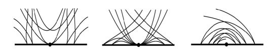
Figure 1. Folded saddle (left), node (center) and focus (right)

In both cases, the topological classification of generic $1$ and $2$-parameter families of BDEs have been established in Bruce-Fletcher-Tari [4, 6] and Tari [22, 23], respectively. We use those results below. Besides, we need a generic $3$-parameter family of BDE studied in Oliver [15].

4.2. BDE of asymptotic curves

Consider the surface locally given by Monge form $(x,y,f(x,y))$ around the origin. Then asymptotic lines are defined by

$$f_{yy}dy^{2}+2f_{xy}dxdy+f_{xx}dx^{2}=0,$$

which we call asymptotic BDE for short. The discriminant is the same as the parabolic curve. We first discuss bifurcations of asymptotic BDE around parabolic and flat umbilic points.

Note that asymptotic BDE’s form a particular class of general BDE’s; the classification of asymptotic BDE is intimately related to the singularity type of the height function (i.e. the Monge form). The parabolic curve can be seen as the locus where the height function has $A_{\geq 2}$-singularities; when the height function has a $A_{3}^{\pm}$-singularity, the surface has an ordinary cusp of Gauss, which corresponds to the type $\Pi^{p}_{c,1}$ – in this case the asymptotic BDE has a folded saddle singularity ($A_{3}^{-}$) and has a folded node or focus singularity ($A_{3}^{+}$). The transitions in $1$-parameter families occur generically in three ways at the following singularities of the height function: non-versal $A_{3}$, $A_{4}$ and $D_{4}$ (flat umbilic) [6]. For $2$-parameter families, $A_{3},$ $A_{4}$, $A_{5}$ and $D_{5}$ singularities of the height function generically appear.

Combining these results with our Theorem 1.1, the following propositions are immediately obtained.

Proposition 4.1.

The following classes in Table 1 correspond to structurally stable types of BDE given in [7, 8, 9].

• $\Pi^{p}_{{\rm I},k}\;(1\leq k\leq 4):$ the parabolic curve is smooth and the unique direction defined by $\delta=0$ is transverse to the curve; the BDE is smoothly equivalent to

  $$dy^{2}+x\,dx^{2}=0.$$

• $\Pi^{p}_{c,1},\;\Pi^{p}_{c,4},\;\Pi^{p}_{c,5}:$ the parabolic curve is smooth and the unique direction defined by $\delta=0$ is tangent to the curve, i.e. it is an ordinary/degenerate cusp of Gauss; the BDE is smoothly equivalent to

  $$dy^{2}+(-y+\lambda x^{2})dx^{2}=0$$

  with $\lambda=6c_{40}-\frac{3}{2}\not=0$, where $c_{40}$ is the coefficient of $x^{4}$ in the normal form.

Proof :  The results follow from the comments in section 4.1 above. If $j^{4}f=y^{2}+x^{2}y+c_{40}x^{4}$, the $2$-jet of the asymptotic BDE is transformed to the above form (below) via $x=\bar{x}$ and $y=-\frac{1}{2}\bar{x}^{2}-\bar{y}$. $\Box$

Remark 4.2.

As $c_{40}=0$ for $\Pi^{p}_{c,4}$ and $\Pi^{p}_{c,5}$, we see $\lambda=-\frac{3}{2}<0$, thus the BDE has a folded saddle at the origin. The folded saddle-node bifurcation (cf. Fig.2 in [22]) occurs at $\lambda=0$. That is the case of $c_{40}=\frac{1}{4}$, that corresponds to the classes $\Pi^{p}_{c,k}\;(k=2,3)$ dealt below. However, another exceptional value $\lambda=\frac{1}{16}$ does not relate to the projection type, i.e. the folded node-forcus bifurcation of asymptotic BDE occurs within the same class $\Pi^{p}_{c,1}$ (cf. Fig.3 in [22]).

Proposition 4.3.

The following classes in Table 1 correspond to some topological types of BDE with codimension $1$.

• $\Pi^{p}_{v,1}:$ the Monge form has an $A_{3}$-singularity at the origin, at which the parabolic curve has a Morse singularity; the BDE is topologically equivalent to the non-versal $A_{3}^{\pm}$-transitions with Morse type 1 in [6]

  $$dy^{2}+(\pm x^{2}\pm y^{2})dx^{2}=0.$$

• $\Pi^{p}_{c,2}:$ the Monge form has an $A_{4}$-singularity at the origin, at which the parabolic curve is smooth ; the BDE is topologically equivalent to the well-folded saddle-node type in [6, 10]

  $$dy^{2}+(-y+x^{3})dx^{2}=0,$$

  provided the coefficient of $x^{5}$ in the normal form $c_{50}\neq 0$.

• $\Pi^{f}_{1}:$ the Monge form has a $D_{4}^{\pm}$-singularity at the origin, at which the parabolic curve has a Morse singularity; the BDE is topologically equivalent to the bifurcation of star/$1$-saddle types in [4]

  $$D_{4}^{+}: ydy^{2}-2xdxdy-ydx^{2}=0\;\;\mbox{\rm(star)};$$

  $$D_{4}^{-}: ydy^{2}+2xdxdy+ydx^{2}=0\;\;\mbox{\rm($1$-saddle)}.$$

Proof :  For $\Pi^{p}_{v,1}$, our conditions $c_{30}=c_{21}=0$ in Table 6 appears in [6, p.501], and also $S\not=0$ if and only if the $2$-jet $j^{2}\delta(0)$ is non-degenrate, hence the normal form follows from Theorem 2.7 (and Prop. 4.1) in [6]. For $\Pi^{p}_{c,2}$, $c_{30}=B=0$ and $A\not=0$ in Table 6 completely coincide with the condition for $A_{4}$-transition in [6, p.502], and the normal form of BDE is immediately obtained (cf. [10]). For the class $\Pi^{f}_{1}$, the asymptotic BDE is given in [4, Cor. 5.3]: indeed, for the normal form of $\Pi^{f}_{1}$, the parabolic curve is defined by $3x^{2}-y^{2}+18\beta xy^{2}+\cdots=0$, hence it has a node at the origin for any parameters $\alpha,\beta$. $\Box$

Proposition 4.4.

The following classes in Table 1 correspond to some topological types of BDE with codimension $\geq 2$. Below $c_{ij}$ are coefficients of the normal form of each class in Table 1.

• $\Pi^{p}_{v,2}:$ the Monge form has an $A_{3}$-singularity at the origin, at which the parabolic curve has a cusp singularity; the BDE is topologically equivalent to the cusp type in [22]

  $$dy^{2}+(\pm x^{2}+y^{3})dx^{2}=0,$$

  provided $\lambda_{1}:=\pm 5c_{50}c_{31}^{3}+12c_{41}c_{31}^{2}\pm 24c_{32}c_{31}+32c_{23}\neq 0$.

• $\Pi^{p}_{v,3}:$ the Monge form has an $A_{4}$-singularity at the origin, at which the parabolic curve has a Morse singularity; the BDE is topologically equivalent to the non-transvese Morse type in [22]

  $$dy^{2}+(xy+x^{3})dx^{2}=0$$

  provided $\lambda_{2}:=c_{31}\neq 0$.

• $\Pi^{p}_{c,3}:$ the Monge form has an $A_{5}$-singularity at the origin, at which the parabolic curve is smooth; the BDE is topologically equivalent to the folded degenerate elementary type in [22]

  $$dy^{2}+(-y\pm x^{4})dx^{2}=0,$$

  provided $\lambda_{3}:=c_{60}-\frac{1}{2}c_{41}\neq 0$.

• $\Pi^{f}_{2}:$ the Monge form has a $D_{5}$-singularity at the origin, at which the parabolic curve has a cusp singularity; the BDE is topologically equivalent to a cusp type 2 in [15]

  $$x^{2}dx^{2}+2ydxdy+xdy^{2}=0.$$

Here $\lambda_{i}$ coincide moduli parameters appearing in the normal forms of jets of BDE studied in [22].

Proof :  For the first three classes, it suffices to check the condition for BDE in Proposition 4.1 of [22]. Indeed, for each of three classes, our condition described in Table 6 of §2.2 and additional conditions described above, $\lambda_{1},\lambda_{2},\lambda_{3}\not=0$, are found in [22, p.156], and the jets of BDE are given there (see Theorem 1.1 of [22] for the normal forms). For $\Pi^{f}_{2}$, as the $1$-jet of the asymptotic BDE is given by $j^{1}(a,b,c)(0)=(2x,2y,0)$ and the parabolic curve is defined by $-4y^{2}+24x^{3}+\cdots=0$, namely it has a cusp at the origin, the result follows from Theorem 3.4 in [15]. $\Box$

Remark 4.5.

In Oliver [15], BDE with the discriminant having a cusp are classified up to codimension $4$, that generalizes a result for cusp types of codimension $2$ in [23]. It is remarkable that the BDE for $\Pi^{f}_{2}$ in Proposition 4.4 is one of such BDE with codimension $3$ in the space of all BDE, while the stratum $\Pi^{f}_{2}$ has codimension $2$ in the space of all Monge forms as seen in Theorem 1.1.

4.3. Bifurcations of parabolic and flecnodal curves

Smooth and topological classifications of BDE do miss the geometry of flecnodal curves, although it is quite fruitful. In part of his dissertation [26] Uribe-Vargas presented 14 types of generic $1$-parameter bifurcations of parabolic and flecnodal curves and of special elliptic points on the surface. That was done by a nice geometric argument using projective duality, however explicit normal forms are not given there. Thus we try to detect substrata in our classification of Monge forms which correspond to Uribe-Vargas’ types.

Each type defines an invariant open subset of one of our class of codimension $3$, or a proper invariant subset of a class of less codimension, which should be characterized by some particular relation of moduli parameters in the normal form. In fact we have already seen 8 types of degenerate parabolic and flat umbilical points in Uribe-Vargas’ list as in all cases in Proposition 4.3 and an exceptional case in Proposition 4.1:

• $\Pi^{p}_{v,1}$ (4 types w.r.t. $\pm x^{4}$ and $\beta\lessgtr\frac{3}{8}\alpha^{2}$ in the normal form);

• $\Pi^{p}_{c,2}$ (the folded saddle-node type);

• $\Pi^{f}_{1}$ (star type and $1$-saddle type);

• $\Pi^{p}_{c,4}$ (degenerate cusp of Gauss).

Remark 4.6.

The corresponding strata in jet space have codimension $3$. Take a generic family of surfaces passing through each stratum. Around a point of class $\Pi^{p}_{v,1}$, Morse bifurcations of the parabolic curve happen, while bifurcations of the flecnodal curve can not be analyzed from the classification of BDE in [6]. Such bifurcations have been determined completely in [26] and can also be checked by direct computations from our Monge forms. For $\Pi^{p}_{c,2}$, two folded saddle points are cancelled at this point, called in [6, Prop. 4.2] the folded saddle-node bifurcation. For $\Pi^{f}_{1}$, there are two types of degenerate flat umbilic points. For $\Pi^{p}_{c,4}$, parabolic and flecnodal curves meet tangentially, and a butterfly point comes across at the cusp of Gauss point. As an additional remark, for $\Pi^{p}_{c,1}$ with $\lambda=\frac{1}{16}$, the folded node-forcus bifurcation of BDE appears as mentioned in Remark 4.2, but the parabolic and flecnodal curves do not bifurcate, so this case is not included.

The rest are divided into 5 types occurred at hyperbolic points and 1 type at an elliptic point; the normal forms for degenerate hyperbolic points are given below:

• $\Pi^{h}_{3,6}$ (degenerate butterfly type);

• $\Pi^{h}_{4,5}$ (swallowtail+butterfly);

• $\Pi^{h}_{3,5}$ with $\alpha=0$ (Morse bifurcation; ‘lips’ and ‘bec-à-bec’);

• $\Pi^{h}_{4,4}$ with $\alpha\beta=16$ (tacnode bifurcation).

In Table 2 (hyperbolic Monge forms), there are two strata of codimension $3$. For the normal form of $\Pi^{h}_{3,6}$, the flecnodal curve is smooth, and the $y$-axis is tangent to the surface with $6$-point contact. Through a generic bifurcation, two butterfly points ($\Pi^{h}_{3,5}$) are cancelled (or created) at this point. For $\Pi^{h}_{4,5}$, there are two irreducible components of the flecnodal curve, one of which has a butterfly at the origin. It bifurcates into one point of $\Pi^{h}_{4,4}$ and one butterfly point.

In strata of codimension $2$, generic bifurcations of flecnodal curves may occur at some particular values of parameters appearing in the normal forms. First consider the class $\Pi^{h}_{3,k}\;(k\geq 4)$: $f(x,y)=xy+x^{3}+\sum_{i+j\geq 4}c_{ij}\,x^{i}y^{j}$ ($\alpha=c_{13}$ in Table 2). We are now viewing the surface along lines close to the $y$-axis, so take parallel projection $\varphi:(x,y)\mapsto(x-uy,f(x,y)-vy)$. The flecnodal curve is just the locus of singular points $(x,y)$ at which the projection for some $(u,v)$ has the swallowtail singularities or more degenerate ones. Put $\lambda:=\det d\varphi$ and $\eta:=u\frac{\partial}{\partial x}+\frac{\partial}{\partial y}$ so that $\eta$ spans the kernel of $d\varphi$ over $\lambda=0$. Then the locus is defined to be the image via projection $(x,y,u,v)\mapsto(x,y)$ of curves given by three equations $\lambda=\eta\lambda=\eta\eta\lambda=0$ (cf. [13]). By $\lambda=0$ we eliminate $v$, and by $\eta\lambda=0$, we solve $u$ by implicit function theorem: $u=-c_{22}x^{2}-3c_{13}xy-6c_{04}y^{2}+o(2)$. Substitute them into $\eta\eta\lambda=0$; we have the expansion of the equation of flecnodal curve:

$$c_{13}x+4c_{04}y+c_{23}x^{2}+4c_{14}xy+10c_{05}y^{2}+h.o.t.=0.$$

The curve is not smooth at the origin when $c_{13}=c_{04}=0$, and it has a Morse singularity if $5c_{23}c_{05}-2c_{14}^{2}\not=0$. Thus, we conclude that Morse bifurcations of flecnodal curves occur at a point of the class $\Pi^{h}_{3,5}$ with $\alpha=0$ and generic homogeneous terms of order $5$ (those are regarded as normal forms for ‘lips’ and ‘bec-à-bec’ in [26]).

Next, consider the class $\Pi^{h}_{4,4}$: $f(x,y)=xy+x^{4}+y^{4}+\alpha xy^{3}+\beta x^{3}y+o(4)$. In entirely the same way as seen above, for each of projections $\varphi_{L}:(x,y)\mapsto(x-uy,f(x,y)-vy)$ and $\varphi_{R}:(x,y)\mapsto(y-ux,f(x,y)-vx)$, we take $\lambda$ and $\eta$, and solve $\lambda=\eta\lambda=\eta\eta\lambda=0$. We then obtain the equation of each component of the flecnodal curve:

$$\alpha x+4y+h.o.t=0,\quad 4x+\beta y+h.o.t=0.$$

Thus the tacnode bifurcation (tangency of two components) occurs at a point of the class $\Pi^{h}_{4,4}$ with $\alpha\beta=16$. The condition exactly coincides with the one in Table 3.2 in Landis [14]. It is also observed that in the elliptic domain, a similar bifurcation occurs at the class $\Pi^{e}_{4,4}$ with a particular value.

References

• [1] V. I. Arnold, Catastrophe Theory, 3rd edition, Springer (2004).
• [2] V. I. Arnold, V. V. Goryunov, O. V. Lyashko, V. A. Vasil’ev, Singularity Theory II, Classification and Applications, Encyclopaedia of Mathematical Sciences Vol. 39, Dynamical System VIII (V. I. Arnold (ed.)), (translation from Russian version), Springer-Verlag (1993).
• [3] J. W. Bruce and F. Tari, Dupin indicatrices and families of curve congruences. Trans. Amer. Math. Soc. 357 (2005), 267-ー85.
• [4] J. W. Bruce and F. Tari, On binary differential equations, Nonlinearity 8 (1995), 255–271.
• [5] J. W. Bruce and F. Tari, Generic $1$-parameter families of binary differential equations of Morse type, Discrete and continuous dynamical systems, 3 (1997), 79–90.
• [6] J. W. Bruce, G. J. Fletcher and F. Tari, Bifurcations of implicit differential equations, Proc. Royal Soc. Edinburgh, 130 A (2000), 485–506.
• [7] M. Cibrario, Sulla reduzione a forma delle equationi lineari alle derviate parziale di secondo ordine di tipo misto, Accademia di Scienze e Lettere, Instituto Lombardo Redicconti, 65, 889-906 (1932).
• [8] L. Dara, Singularités génériques des équations differentielles multiformes, Bol. Soc. Brasil Math. 6 (1975), 95–128.
• [9] A. A. Davydov, Normal form of a differential equation, not solvable for the derivative, in a neighborhood of a singular point, Funct. Anal. Appl. 19 (1985), 1–10.
• [10] A. A. Davydov and E. Rosales-Gonsales, Smooth normal forms of folded elementary singular points, Jour. Dyn. Control Systems 1 (1995), 463–482.
• [11] J. L. Deolindo-Silva, Y. Kabata, Projective classification of jets of surfaces in $\mathbb{P}^{4}$ and applications, preprint (2015).
• [12] V.V. Goryunov, Singularities of projections of complete intersections, J. Soviet Math. 27 (1984), 2785–2811.
• [13] Y. Kabata, Recognition of plane-to-plane map-germs, preprint (2015), ArXiv: 1503.08544.
• [14] E. E. Landis, Tangential singularities, Funt. Anal. Appl. 15 (1981), 103–114 (translation).
• [15] J. M. Oliver, Binary differential equations with discriminant having a cusp singularity, Jour. Dyn. Control Systems, 17 (2) (2011), 207–230.
• [16] P. J. Olver, Equivalence, Invariants and Symmetry, Cambridge Univ. Press (1995).
• [17] O. A. Platonova, Singularities of the mutual disposition of a surface and a line, Uspekhi Mat. Nauk, 36:1 (1981), 221–222.
• [18] O. A. Platonova, Projections of smooth surfaces, J. Soviet Math. 35 no.6 (1986), 2796–2808
• [19] J. H. Rieger, Families of maps from the plane to the plane, J. London Math. Soc. 36 (1987), 351–369.
• [20] J. H. Rieger, Versal topological stratification and the bifurcation geometry of map-germs of the plane, Math. Proc. Cambridge Phil. Soc. 107, no. 1, (1990), 127-147.
• [21] J. H. Rieger, The geometry of view space of opaque objects bounded by smooth surfaces, Artificial Intelligence. 44 (1990), 1-40.
• [22] F. Tari, Two parameter families of implicit differential equations, Discrete and continuous dynamical systems, 13 (2005), 139–262
• [23] F. Tari, Two parameter families of binary differential equations, Discrete and continuous dynamical systems, 22 (3) (2008), 759–789.
• [24] A. Tresse, Sur les invariants des groupes continus de transformations, Acta Math. 18 (1894), 1–88.
• [25] R. Uribe-Vargas, A projective invariant for swallowtails and godrons, and global theorems on the flecnodal curve, Mosc. Math. J., 6 (2006), 731–772.
• [26] R. Uribe-Vargas, Surface evolution, implicit differential equations and pairs of Legendrian fibrations, preprint.
• [27] J. West, The Differential Geometry of the Cross-Cap, Dissertation, University of Liverpool (1995).
• [28] E. J. Wilczynski, Projective Differential Geometry of Curved Surfaces, Trans. Amer. Math. Soc. 10 (1909), 279–296.
• [29] T. Yoshida, Y. Kabata and T. Ohmoto, Bifurcations of plane-to-plane map-germs of corank $2$, Quarterly J. Math. (2014) doi:10.1093/qmath/hau013.
• [30] T. Yoshida, Y. Kabata and T. Ohmoto, Bifurcations of plane-to-plane map-germs of corank $2$ of parabolic type, to appear in RIMS koukyuroku Bessatsu (2015).