Tunneling spectroscopy and Josephson current of superconductor-ferromagnet hybrids on the surface of a 3D TI

Abstract

We investigate the charge transport property of superconductor (S) /normal metal (N) / ferromagnet insulator (FI) /(normal metal) N’ and S/N/FI/N’/S Josephson junctions on a three-dimensional topological insulator surface. We find the asymmetric local density of states (LDOSs) in a S/N/FI/N’ junction and show that the N interlayer gives rise to subgap resonant spikes in the differential conductance and LDOSs. In a S/N/FI/N’/S junction, the Josephson current shows a non-sinusoidal current-phase relation and the N (or N’) interlayer decreases the magnitude of the critical current monotonically.

I I. Introduction

Three dimensional (3D) topological insulator (TI) is a phase of matter with topologically protected Dirac-type surface states on their time reversal invariant point Fu07prb ; Hsieh08 ; Hsieh09 ; Hasan09 ; ZSC09 ; Chen09 ; Xia09 ; Ando10 ; KaneReview ; MooreReview ; ZhangReview ; AndoReview . With coupling to a ferromagnet (F), Dirac fermions show many exotic properties such as magnetoelectric effect Qi08prb ; Qi08np ; Moore09 ; MacD10 ; Franz10 ; Nomura11 . By the proximity effect to a superconductor (S), the 3D TI surface states may become a topological superconductor Kane2008 . When F and S coexist on 3D TI surfaces, it is found that chiral Majorana edge states can be generated at the boundary between them Kane2008 ; Kane2009 ; Beenakker09 , which leads to the formation of zero-biased conductance peak (ZBCP) TK95 as experimental signaturesTanaka2009 ; BeenakkerReview ; AliceaReview ; Tanakareview ; Snelder15 . Intrinsic topological superconductivity has also been found in doped 3D TIs, e.g., Cu_xBi₂Se₃ hor10 ; 097001 ; Sasak11 ; Kriener11 ; levy13 .

On the other hand, a variety of interesting phenomena about Josephson effect in TI materials have been discovered Zhang11 ; Sacepe ; Brinkman ; Williams ; Wang12 ; Snelder14 ; Moler15 . Recently, a non-sinusoidal current-phase relation has been reported in the 3D TI HgTe junction Moler15 . In the 3D TI heterojunctions like Nb/Bi_1.5Sb_0.5Te_1.7Se_1.3/Nb, the temperature dependence of the critical current is almost linear in most of the range Snelder14 . Also, the novel Josephson effect involving Majorana fermions has been predicted theoretically Tanaka2009 ; Linderprl10 ; Linderprb10 ; Yokoyama12 ; Snelder13 , however, there has been no experimental report yet. The rapid development in experiments requires for a theoretical approach which can deal with realistic structures for Josephson junctions on 3D TI surface.

In this article, we address how to compose Green’s function by wave functions on superconducting 3D TI surface. Using the resulting formalism, one can analyze the spacial dependence of physical quantities, such as local density of states (LDOSs) and pair potentials. Also, this approach provides an efficient way to calculate Josephson current for realistic junctions on 3D TI surfaces. In this work, we consider the S/normal metal (N)/ferromagnetic insulator (FI)/N’ junction and S/N/FI/N’/S Josephson junction as examples. Since making direct contact between F and S regions is not easily accessible in actual experiments, the presence of N interlayer between S and F is a more realistic setup to study Majorana fermions. In the S/N/FI/N’ junction, we find that the conductance spectra and LDOSs have spikes as a function of bias voltage and quasiparticle energy $E$, respectively. The resulting LDOSs shows an asymmetric energy dependence around $E=0$ . For the S/N/FI/N’/S junction, we find that the distance of N interlayer (or N’ interlayer) decreases the critical current monotonically. The junctions with or without FI show a non-sinusoidal current-phase relation at low temperatures.

The paper is organized as follows: In section II, we introduce our model and construct the Green’s function. In section III, we show numerical results for S/N/FI/N’ and S/N/FI/N’/S junctions and discuss them. A conclusion remark is given in Section IV.

II II. Model

We consider the ballistic S/N/FI/N’ and S/N/FI/N’/S junctions which are shown in Fig.1.

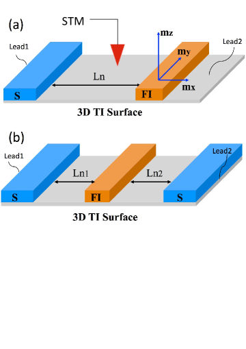
Figure 1: Schematics of the system: (a) S/N/FI/N’ and (b) S/N/FI/N’/S formed on the surface of a 3D topological insulator. The local density of states can be detected by the STM tip. The differential conductance and the suppercurrent can be obtained from the leads on the two sides.

The system can be described by the BdG Hamiltonian BdG ; Tanaka2009

$$\hat{H}=\left[\begin{array}[]{cc}h(k_{x},k_{y})+M&i\hat{\sigma}_{y}\Delta\\ -i\hat{\sigma}_{y}\Delta^{\ast}&-h^{\ast}(-k_{x},-k_{y})-M^{\ast}\end{array}\right],$$ (1)

in $\left(\Psi_{\uparrow},\Psi_{\downarrow},\Psi_{\uparrow}^{{\dagger}},\Psi_{\downarrow}^{{\dagger}}\right)^{T}$ basis, where $h(k_{x},k_{y})=v_{f}(k_{y}\hat{\sigma}_{x}-k_{x}\hat{\sigma}_{y})-\mu(\Theta\left(-x+L_{n\left(n1\right)}\right)+\Theta\left(x-L_{n\left(n1\right)}-L_{f}\right))$ for the S/N/FI/N’ (S/N/FI/N’/S) junction. $\hat{\sigma}_{i=x,y,z}$ are the Pauli matrices in the spin space and $\mu$ is the chemical potential. Throughout the paper, we set $\hbar=1$. The exchange field in F region is $M=\sum_{i=x,y,z}m_{i}\hat{\sigma}_{i}\Theta\left(x-L_{n\left(n1\right)}\right)\Theta\left(L_{n\left(n1\right)}+L_{f}-x\right)$ for the S/N/FI/N’ (S/N/FI/N’/S) junction. The pair potential $\Delta$ is given by $\Delta_{0}\Theta(-x)$ for the S/N/FI/N’ junction and $\Delta_{0}[\Theta(-x)+e^{-i\phi}\Theta(x-L_{n1}-L_{f}-L_{n2})]$ for the S/N/FI/N’/S junction, where $\phi$ is the macroscopic superconducting phase.

In this article, we use a standard formula of tunneling spectroscopy BTK ; TK95 as shown in Ref.Tanaka2009 to obtain differential conductance spectra of the S/N/FI/N’ junction. Here, we would like to present the way of constructing the retarded Green’s function which has recently been applied to relativistic system like Graphene Asano08 ; Burst10 , and 1D helical states on TI Pablo15 . In our system, the translational invariance along the $y$-axis is preserved, thus the retarded Green’s function with respect to Eq.1 has the form $\check{G}(x,x^{\prime},y,y^{\prime})=\sum\nolimits_{k_{y}}G^{k_{y}}(x,x^{\prime})e^{ik_{y}(y-y^{\prime})}$. The retarded Green’s function can be written as McMillan ; FT ; TanakaD ; Tanaka2000 ; Burst10

$$\begin{array}[]{r}G^{k_{y}}(x,x^{\prime})=\alpha_{1}\psi_{1}(x)\tilde{\psi}_{3}^{T}(x^{\prime})+\alpha_{2}\psi_{1}(x)\tilde{\psi}_{4}^{T}(x^{\prime})\\ +\alpha_{3}\psi_{2}(x)\tilde{\psi}_{3}^{T}(x^{\prime})+\alpha_{4}\psi_{2}(x)\tilde{\psi}_{4}^{T}(x^{\prime}),\end{array}$$ (2)

for $x>x^{\prime}$ and

$$\begin{array}[]{r}G^{k_{y}}(x,x^{\prime})=\beta_{1}\psi_{3}(x)\tilde{\psi}_{1}^{T}(x^{\prime})+\beta_{2}\psi_{4}(x)\tilde{\psi}_{1}^{T}(x^{\prime})\\ +\beta_{3}\psi_{3}(x)\tilde{\psi}_{2}^{T}(x^{\prime})+\beta_{4}\psi_{4}(x)\tilde{\psi}_{2}^{T}(x^{\prime}),\end{array}$$ (3)

for $x<x^{\prime}$. $\psi_{i=1\sim 4}\left(x\right)$ are wave functions of Eq.(1) with wave vector $k_{y}$. $\psi_{1(2)}(x)$ is the wave function for an incident electron-like (hole-like) particle from the left side. $\psi_{3(4)}(x)$ is the wave function for the incident electron-like (hole-like) particles from the right side. $\tilde{\psi}_{i=1\sim 4}(x^{\prime})$ are the wave functions corresponding to the conjugate processes under the Hamiltonian

$$\tilde{H}=\left[\begin{array}[]{cc}\tilde{h}(k_{x},k_{y})+M^{\ast}&i\sigma_{y}\Delta^{\ast}\\ -i\sigma_{y}\Delta&-\tilde{h}^{\ast}(-k_{x},-k_{y})-M\end{array}\right]$$ (4)

with wave vector $-k_{y}$ and $\tilde{h}(k_{x},k_{y})$ is given by $\tilde{h}(k_{x},k_{y})=v_{f}(-k_{y}\sigma_{x}-k_{x}\sigma_{y})-\mu[\Theta(-x+d_{n1})+\Theta(x-d_{n1}-d_{f})]$. For example, in the left S side, the wave functions are

$$\psi_{1}(x)=\hat{A}_{1}e^{ik_{+}x}+a_{1}\hat{A}_{4}e^{ik_{-}x}+b_{1}\hat{A}_{3}e^{-ik_{+}x},$$ (5a)

$$\psi_{2}(x)=\hat{A}_{2}e^{-ik_{-}x}+a_{2}\hat{A}_{3}e^{-ik_{+}x}+b_{2}\hat{A}_{4}e^{ik_{-}x},$$ (5b)

$$\psi_{3}(x)=c_{3}\hat{A}_{3}e^{-ik_{+}x}+d_{3}\hat{A}_{4}e^{ik_{-}x},$$ (5c)

$$\psi_{4}(x)=c_{4}\hat{A}_{4}e^{ik_{-}x}+d_{4}\hat{A}_{3}e^{-ik_{+}x},$$ (5d)

and

$$\tilde{\psi}_{1}(x^{\prime})=\hat{B}_{1}e^{ik_{+}x^{\prime}}+\tilde{a}_{1}\hat{B}_{4}e^{ik_{-}x^{\prime}}+\tilde{b}_{1}\hat{B}_{3}e^{-ik_{+}x^{\prime}},\newline$$ (6a)

$$\tilde{\psi}_{2}(x^{\prime})=\hat{B}_{2}e^{-ik_{-}x^{\prime}}+\tilde{a}_{2}\hat{B}_{3}e^{-ik_{+}x^{\prime}}+\tilde{b}_{2}\hat{B}_{4}e^{ik_{-}x^{\prime}},\newline$$ (6b)

$$\tilde{\psi}_{3}(x^{\prime})=\tilde{c}_{3}\hat{B}_{3}e^{-ik_{+}x^{\prime}}+\tilde{d}_{3}\hat{B}_{4}e^{ik_{-}x^{\prime}},\newline$$ (6c)

$$\tilde{\psi}_{4}(x^{\prime})=\tilde{c}_{4}\hat{B}_{4}e^{ik_{-}x^{\prime}}+\tilde{d}_{4}\hat{B}_{3}e^{-ik_{+}x^{\prime}}.$$ (6d)

The corresponding wave vectors are represented by $$k_{\pm}=\sqrt{(\mu\pm\sqrt{E^{2}-\Delta_{0}^{2}})^{2}/v_{f}^{2}-k_{y}^{2}}\equiv q_{e(h)}\cos\theta_{\pm} q_{e(h)}=(\mu\pm\sqrt{E^{2}-\Delta_{0}^{2}})/v_{f}$$ and . The spinors are given as

$$\hat{A}_{1}(\hat{B}_{3}) = [iu,\pm e^{\pm i\theta_{+}}u,\mp e^{\pm i\theta_{+}}v,iv]^{T},$$ (7a)

$$\hat{A}_{2}(\hat{B}_{4}) = [ie^{\pm i\theta_{-}}v,\mp v,\pm u,ie^{\pm i\theta_{-}}u]^{T},$$ (7b)

$$\hat{A}_{3}(\hat{B}_{1}) = [ie^{\pm i\theta_{+}}u,\mp u,\pm v,ie^{\pm i\theta_{+}}v]^{T},$$ (7c)

$$\hat{A}_{4}(\hat{B}_{2}) = [iv,\pm e^{\pm i\theta_{-}}v,\mp e^{\pm i\theta_{-}}u,iu]^{T},$$ (7d)

where $$u v u(v) = \sqrt{(E\pm\sqrt{E^{2}-\Delta_{0}^{2}})/2E} a_{i} b_{i} \tilde{a}_{i} \tilde{b}_{i} \psi_{i}(x=0_{+})=\psi_{i}(x=0_{-}) \psi_{i}(x=d_{n+})=\psi_{i,}(x=d_{n-}) \psi_{i}(x=d_{n}+d_{f+})=\psi_{i}(x=d_{n}+d_{f-}) \alpha_{i=1\sim 4} \beta_{i=1\sim 4}$$ and are given by . Other wave functions can be found in the Appendix. The coefficients , , and can be solved from the boundary condition for relativistic systems. For example, in S/N/FI/N’ junction, the boundary conditions are: , , , and similar to other processes. and can be determined by the boundary conditions of Green’s function

$$G^{k_{y}}(x+0,x)-G^{k_{y}}(x-0,x)=v_{f}^{-1}(i\hat{\tau}_{z}\hat{\sigma}_{y}),$$ (8)

where $\hat{\tau}_{i=x,y,z}$ are the Pauli matrices in the electron-hole space. In real materials, the magnitude of the superconducting gap is much smaller than the chemical potential $\Delta_{0}\sim 10^{-3}\mu$, so we can use the quasiclassical approximation as $q_{e}\sim q_{h}$ and $\theta_{+}\sim\theta_{-}\equiv\theta$. Then one can easily obtain the values of $\alpha_{i=1\sim 4}$ and $\beta_{i=1\sim 4}$,

$$\alpha_{1(4)} = [2iv_{f}\cos\theta(u^{2}-v^{2})(\tilde{d}_{3}\tilde{d}_{4}-\tilde{c}_{3}\tilde{c}_{4})]^{-1}\tilde{c}_{4(3)},$$ (9a)

$$\alpha_{2(3)} = [2iv_{f}\cos\theta(u^{2}-v^{2})(\tilde{c}_{3}\tilde{c}_{4}-\tilde{d}_{3}\tilde{d}_{4})]^{-1}\tilde{d}_{3(4)},$$ (9b)

$$\beta_{1(4)} = [2iv_{f}\cos\theta(u^{2}-v^{2})(d_{3}d_{4}-c_{3}c_{4})]^{-1}c_{4(3)},$$ (9c)

$$\beta_{2(3)} = [2iv_{f}\cos\theta(u^{2}-v^{2})(c_{3}c_{4}-d_{3}d_{4})]^{-1}d_{3(4)}.$$ (9d)

From the Green’s function, we can obtain the local density of states for electrons: $$\rho_{e}(x,E) \rho_{h}(x,E)$$ and that for holes: ,

$$\rho_{e\left(h\right)}(x,E)=\rho_{e\left(h\right),\uparrow}(x,E)+\rho_{e\left(h\right),\downarrow}(x,E),$$ (10)

where the spin-resolved LDOSs are given by

$$\rho_{e,\uparrow\left(\downarrow\right)}(x,E) = -\frac{1}{\pi}\sum_{k_{y}}\mathrm{Im}[G_{11\left(22\right)}^{k_{y}}(x,x,E)],$$ (11)

$$\rho_{h,\uparrow\left(\downarrow\right)}(x,E) = -\frac{1}{\pi}\sum_{k_{y}}\mathrm{Im}[G_{33\left(44\right)}^{k_{y}}(x,x,E)].$$ (12)

The dc Josephson current is determined by electric charge conservation rule

$$\partial_{t}P+\partial_{x}J_{x}+S=0,$$ (13)

where $P=\Psi_{\uparrow}^{{\dagger}}\Psi_{\uparrow}+\Psi_{\downarrow}^{{\dagger}}\Psi_{\downarrow}$, $J_{x}=iv_{f}(\Psi_{\uparrow}^{{\dagger}}\Psi_{\downarrow}-\Psi_{\downarrow}^{{\dagger}}\Psi_{\uparrow})$ and $S=2\mathrm{Im}[\Delta^{\ast}\Psi_{\downarrow}\Psi_{\uparrow}-\Delta^{\ast}\Psi_{\uparrow}\Psi_{\downarrow}]$ are electric charge density, electric current and source term, respectively. After straightforward calculations following Ref.FT ; Tanaka2000 , we find that the total Josephson current is

$$J_{x}=ek_{B}T\sum_{k_{y},\omega_{n}}\frac{\Delta}{2}\frac{\mathrm{sgn}(\omega_{n})}{\sqrt{\omega_{n}^{2}+\Delta^{2}}}\left[a_{1}(i\omega_{n})-a_{2}(i\omega_{n})\right],$$ (14)

where $\omega_{n}$ is the Matsubara frequency $\omega_{n}=\pi k_{B}T(2n+1),(n=0,\pm 1,\pm 2....)$. Eq.(14) shows that Furusaki-Tsukada’s formula FT can also be applicable to the ballistic Dirac-like electron systems on 3D TI surfaces Benj ; bYang . It enables us to directly calculate the dc Josephson current in even more complicated or long Josephson junctions on 3D TI surface without starting from the energy levels of Andreev bound states Tanaka2009 ; Tkachov .

III III. Numerical Results

III.1 A. S/N/FI/N’ junction

First, we show the conductance $\sigma_{s}$ (see Appendix) of S/N/FI/N’ junction in Fig.2. We normalized $\sigma_{s}$ by $\sigma_{n}$ which is the conductance when S is in normal state. We only consider the exchange field along $z-$ and $x-$axis since the magnetization along $y-$axis does not change the conductance Tanaka2009 . The length of the N layer between S and FI is denoted by $L_{n}$. The direct contact between S and FI means $L_{n}=0$. For sufficient large $m_{z}(m_{x})$, the normalized conductance has a ZBCP similar to that in chiral $p$-wave superconductor Tanaka2009 when magnetic field is along $z$-axis as shown in Fig.2(a). Also we can see from Fig.2(b), ZBCP appears when the magnetization is along $x-$axis. As $L_{n}$ increases, the sub-gap resonant peaks show up (Figs.2(c)$\sim$(f)). The number of such peaks grows with $L_{n}$.

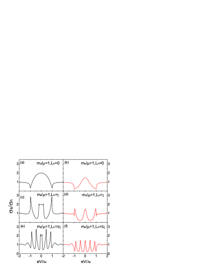
Figure 2: Normalized tunneling conductance as a function of bias voltage $(eV/\Delta_{0})$ for S/N/FI/N’ junctions. (a), (b): $L_{n}=0$, (c), (d): $L_{n}=\xi$ and (e), (f): $L_{n}=3\xi$. Black curve: $m_{z}/\mu=1$ and red curve: $m_{x}/\mu=1$. $\mu_{=}1$, $v_{f}$=1, $\Delta_{0}=0.001$ and $L_{f}=0.001\xi$ are chosen for all the panels.

This oscillatory phenomenon can also be seen in the local density of states $\rho_{e(h)}\left(x,E\right)$. We normalize $\rho_{e(h)}\left(x,E\right)$ to that of the electron density of states of the bulk normal metal $\rho_{n}$ at Fermi energy. Here, we choose the position in the middle of FI $x_{0}=L_{f}/2+L_{n}$ and show the density of states in Fig.3. When $L_{n}\neq 0$, we obtain the subgap peaks again as shown in Fig.3(c $\sim$ f). The formation of such peaks can be explained as follows. We know that the wave vector for electron (hole) is $k_{n}^{\pm}=\sqrt{(\mu\pm E)^{2}/v_{f}^{2}-k_{y}^{2}}$. The condition of forming the Andreev bound states in the N layer can be estimated from the Bohr-Sommerfeld quantization condition as

$$e^{i(k_{n}^{+}-k_{n}^{-})L_{n}}=1,$$ (15)

which shows that the number of peaks is proportional to $L_{n}$. Similar formation of Andreev bound states was also revealed in junctions with 1D helical edge statesCrepin .

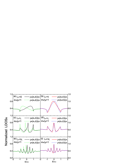
Figure 3: Local density of states in the middle of FI in the S/N/FI/N’ junctions as a function of energy $(E/\Delta_{0})$: (a), (b): $L_{n}=0$, (c), (d): $L_{n}=\xi$ and (e),(f):$L_{n}=3\xi$. Solid line for electron density of states and dashed line for hole density of states. Other parameters are chosen as the same as in Fig.2.

We also find the asymmetric $E$ dependence of LDOSs near the S/FI interface, e.g., $\rho_{e}\left(x_{0},E\right)$($\rho_{h}\left(x_{0},E\right)$) in Fig.3. The asymmetry becomes prominent when magnetization is along $z$ axis (Figs.3(a), (c) and (e)). We know that $\rho_{e}\left(x,E\right)$ and $\rho_{h}\left(x,E\right)$ are symmetric functions of $E$ for chiral $p$-wave superconductor when $\Delta_{0}$ is much smaller than $\mu$ Sigrist . In that case, the time-reversal symmetry is already broken in the bulk states of $p$-wave superconductor. On the other hand, the superconductor on TI is time-reversal invariant and can not support chiral edge mode without attaching ferromagnet. Therefore, we can imagine that the chiral edge mode studied here has a nature similar to Shiba-type bound states Yu ; Shiba ; Rusinov by magnetic impurity scattering.

In usual case, where the spin degree of freedom is degenerate, the emerging Shiba-states still follow the relation $\rho_{e\left(h\right)}(x,E)=\rho_{e\left(h\right)}(x,-E)$, although the decomposed LDOS in each spin sector $\rho_{e\left(h\right),\sigma}(x,E)$ does not satisfy $\rho_{e,\sigma}(x,E)=\rho_{e,\sigma}(x,-E)$. Since $\rho_{e\left(h\right),\sigma}(x,E)=\rho_{e\left(h\right),-\sigma}(x,-E)$ is satisfied, after summing up each spin component, $\rho_{e\left(h\right)}(x,E)=\rho_{e\left(h\right),\uparrow}(x,E)+\rho_{e\left(h\right),\downarrow}(x,E)=\rho_{e\left(h\right),\downarrow}(x,-E)+\rho_{e\left(h\right),\uparrow}(x,-E)=\rho_{e\left(h\right)}(x,-E)$ is satisfied. Then, the resulting LDOS is symmetric around $E=0$. On the other hand, if the spin degeneracy is lifted in the superconductor, it is possible that the LDOS becomes asymmetric. In the present case, there is a strong spin-momentum locking in the superconducting region by spin-orbit coupling. Then the asymmetric energy dependence of $\rho_{e\left(h\right)}(x,E)$ appears near the S/FI interface. In recent experiment of scanning tunneling spectroscopy (STS), similar asymmetric behavior of LDOSs has been observed in 1D S/F systemPerge2014 . We can regard our finding in Fig. 3 as another example of asymmetric LDOSs in planar S/F junction which can be detected in STS.

To see the spacial dependence of the Majorana states in such junctions, we show the zero energy density of states $\rho_{e}(x,E=0)$ throughout the junction. Because $\rho_{e}(x,E=0)$ is $0$ in both isolated S and FI region, significant enhancement of $\rho_{e}(x,E=0)$ in S/FI interface of S/FI/N junction can be regarded as the experimental signature of chiral Majorana fermion. In the S region, we can estimate that the characteristic length expressing the spatial change of $\rho_{e}(x,E=0)$ is the order of macroscopic length scale: $\xi$. This means a sufficient possibility to detect the presence of Majorana fermion experimentally by STS, since the manipulation of tip of STS just on the the S/N or S/F boundary with high resolution is not easy. Also, as seen in Fig.4(b), even if there is a normal layer between S and FI, the enhancement of $\rho_{e}(x,E=0)$ in both F and S is not affected. In the N layer between S and FI, $\rho_{e}(x,E=0)$ is almost constant. In the right N layer, we find oscillations of $\rho_{e}(x,E=0)$ on the scale of the inverse Fermi momenta. However, this oscillatory behavior may be difficult to be detected in actual experiment.

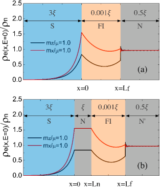
Figure 4: Spacial dependence of zero energy states in (a) S/FI/N junction and (b) S/N/FI/N’ junction. The width of F layer is $L_{f}=0.001\xi$ and that of the N layer in (b) is $L_{n}=\xi$. Other parameters are the same as in Fig.2. The scale of the horizontal axis is different in each region.

III.2 B. Josephson effect

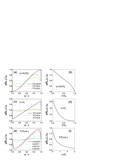
Figure 5: S/N/S Josephson junction: (a) Current-phase relation and (b) critical current for $L_{n}=0.01\xi$. (c) and (d) are those for $L_{n}=\xi$. Length dependence of $L_{n}$ for $T=0.1T_{c}$: (e) current-phase relation and (f) critical current. Other parameters are chosen as the same as in Fig.2.

Before discussing the S/N/FI/N’/S junction, let us first look at S/N/S junction. Using Eq.(14), we plot the dc Josephson current in Fig.5. It is normalized to $eR_{N}J/\Delta_{0}$ where $R_{N}$ is the interface resistance per unit area in the normal state. In panel (a), we can see that the current-phase relation is non-sinusoidal for short-junction in low temperature. This characteristic remains in the long-junction, as shown in panel (c). We notice that in recent experiment of Nb/3D-HgTe/Nb Josephson junctions, the current-phase relation is found to be non-sinusoidal Moler15 . The experimental condition corresponds to low temperature and long-junction in our calculation. We find a similar result in that limit as shown in (c). The temperature dependence of critical current $J_{c}$ for short and long circumstances are given in panel (b) and (d), respectively. We observe that for high temperature, $J_{c}$ is a concave function of $T$ at small $L_{n}$ while it becomes a convex function with large $L_{n}$. It is also interesting to notice that in the large area of low temperature, $J_{c}$ is nearly a linear function of $T$ in both short- and long-junction. This result is in good agreement with the recent experiments in long Nb/Bi_1.5Sb_0.5Te_1.7Se_1.3/Nb Josephson junction Snelder14 . In Figs.5(e) and (f), we plot the length dependence of Josephson current.

We now consider S/N/FI/N’/S Josephson junctions. The length of N layer on the two side of FI is denoted as $L_{n1}$ and $L_{n2}$. When $L_{n1}$ and $L_{n2}$ is on the superconducting coherence length scale, the junctions become long-junctions. The influence of N layer between FI and S is shown in Fig.6. From Figs.6(a) and (b), we can see that the current-phase relation still retains the non-sinusoidal shape for different values of $L_{n1}$ and $L_{n2}$ in low temperature limit. Throughout our study, we have not found the sawtooth behavior of current-phase relation involving magnetization in the long junction and low temperature limit, as shown in Fig.5(c). This is because the magnetization makes the Andreev bound states gapped for most values of $k_{y}$ Tanaka2009 . The derivative of energy dispersion which creates Josephson current will be a smoother function of phase than that in S/N/S junction. For the temperature dependence of the critical current, we can see that it behaves qualitatively different in low temperature limit for $m_{z}$ and $m_{x}$ as shown in Figs.6(c) and (d), respectively. For $m_{z}$ case, the critical current $J_{c}$ saturates at a constant value, which has been revealed by the previous work Linderprb10 . However, for the $m_{x}$ case, it shows a Kulik-Ome’lyanchuk type of critical current KO which has linear low-temperature behavior. We interpret it as a result of the enhanced zero-energy LDOSs for $m_{x}$ magnetization as illustrated in Figs.3(b)(d)(f). In the high temperature limit, it is shown that for both $m_{z}$ and $m_{x}$ cases, $J_{c}$ is a concave function while it crosses over to a convex function with increasing $L_{n1}$ (or $L_{n2}$). This behavior is similar to the S/N/S junction. Figures.6(e) and (f) represent the critical current as a function of the length $L_{n1}$ and $L_{n2}$, for different direction of magnetization.

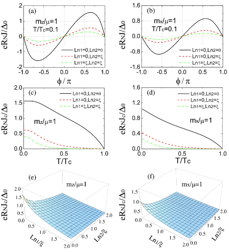
Figure 6: S/N/FI/N’/S junction: current-phase relation for 3 cases of the N layer length $L_{n1}$ and $L_{n2}$ for (a) $m_{z}/\mu=1$ and (b) $m_{x}/\mu=1$. (c)(d) Temperature dependence of critical current corresponding to (a) and (b), respectively. (e)(f) Critical Josephson current as a function of $L_{n1}$ and $L_{n2}$. The temperature is chosen as $T=0.1T_{c}$. Other parameters are chosen as the same as in Fig.5.

It is worth noting that, although the interlayer N in the S/N/FI/N’ junction could generate resonant spikes in the transport phenomena, e.g., spikes in Figs.2 and 3, we find no oscillatory behavior in either current-phase relation or critical current as a function of length N (or N’). The critical current decreases monotonically with the length $L_{n1}+L_{n2}$.

IV IV. SUMMARY

In summary, we theoretically studied the S/N/FI/N’, S/N/S and S/N/FI/N’/S junctions on the surface of 3D topological insulator. We have constructed a formula to obtain Green’s function. The conductance spectra and local density of states in S/N/FI/N’ junction show resonant spikes due to the Andreev bound states. The calculated current phase relation and temperature dependence of critical current in the Josephson junctions are consistent with recent experiments in S/N/S junction. We have also calculated current phase relation and temperature dependence of critical current in S/N/FI/N’/S junction. The non-sinusoidal current phase relation can be expected for short junctions. We hope the obtained results will be confirmed by experiments in the near future.

V ACKNOWLEDGEMENTS

We thank V.V. Ryazanov, A.A. Golubov, Y. Asano and M. Sato for valuable discussions. This work was supported in part by Grants-in-Aid for Scientific Research from the Ministry of Education, Culture, Sports, Science and Technology of Japan (Topological Quantum Phenomena No.22103005 and No.25287085), by the German-Japanese research unit FOR1483 on ”Topotronics”, and by the Ministry of Education and Science of the Russian Federation Grant No.14Y.26.31.0007.

VI APPENDIX: WAVE FUNCTIONS

The wave functions in the N interlayer are

$$\psi_{i}(x) = \sum\limits_{\lambda=1}^{4}s_{\lambda}^{i}\hat{N}_{\lambda}e^{ik_{n,\lambda}x},$$ (16)

$$\tilde{\psi}_{i}(x) = \sum\limits_{\lambda=1}^{4}\tilde{s}_{\lambda}^{i}\hat{N}_{\lambda}e^{ik_{n,\lambda}x},$$ (17)

where

$$\hat{N}_{1\left(2\right)} = \left[v_{f}\left(ik_{n,1\left(2\right)}+k_{y}\right),\mu+E,0,0\right]^{T},$$ (18)

$$\hat{N}_{3\left(4\right)} = \left[0,0,v_{f}\left(ik_{n,3\left(4\right)}-k_{y}\right),-\mu+E\right]^{T},$$ (19)

with

$$k_{n,1\left(2\right)} = \pm\sqrt{(\mu+E)^{2}/v_{f}^{2}-k_{y}^{2}}=\pm k_{n}^{+},$$ (20)

$$k_{n,3\left(4\right)} = \pm\sqrt{(\mu-E)^{2}/v_{f}^{2}-k_{y}^{2}}=\pm k_{n}^{-}.$$ (21)

For the FI interlayer, we find that

$$\psi_{i}(x) = \sum_{\lambda=1}^{4}f_{\lambda}^{i}\hat{F}_{\lambda}e^{ik_{\lambda}^{f}x},$$ (22)

$$\tilde{\psi}_{i}(x) = \sum_{\lambda=1}^{4}\tilde{f}_{\lambda}^{i}\hat{F}_{\lambda}e^{ik_{\lambda}^{f}x},$$ (23)

where

$$\hat{F}_{1} =\left[iv_{f}k_{1}^{f}+\left(v_{f}k_{y}+m_{x}\right),E-m_{z},0,0\right]^{T},$$ (24a)

$$\hat{F}_{2} =\left[E+m_{z},-iv_{f}k_{2}^{f}+\left(v_{f}k_{y}+m_{x}\right),0,0\right]^{T},$$ (24b)

$$\hat{F}_{3} =\left[0,0,-iv_{f}k_{3}^{f}+\left(v_{f}k_{y}-m_{x}\right),E+m_{z}\right]^{T},$$ (24c)

$$\hat{F}_{4} =\left[0,0,E-m_{z},iv_{f}k_{4}^{f}+\left(v_{f}k_{y}-m_{x}\right)\right]^{T},$$ (24d)

with

$$k_{1}^{f}=-\varsigma_{1}\sqrt{E^{2}-m_{z}^{2}-\left(v_{f}k_{y}+m_{x}\right)^{2}},\newline$$ (25a)

$$k_{2}^{f}=\varsigma_{1}\sqrt{E^{2}-m_{z}^{2}-\left(v_{f}k_{y}+m_{x}\right)^{2}},$$ (25b)

$$k_{3}^{f}=\varsigma_{2}\sqrt{E^{2}-m_{z}^{2}-\left(v_{f}k_{y}-m_{x}\right)^{2}},\newline$$ (25c)

$$k_{4}^{f}=-\varsigma_{2}\sqrt{E^{2}-m_{z}^{2}-\left(v_{f}k_{y}-m_{x}\right)^{2}},$$ (25d)

and $$\varsigma_{1\left(2\right)}=\mathrm{sgn}\left(v_{f}k_{y}\pm m_{x}\right)$$. The wave functions in the N’ region of S/N/FI/N’ are

$$\psi_{1}(x)=c_{1}\hat{C}_{1}e^{ik_{n}^{+}x}+d_{1}\hat{C}_{2}e^{-ik_{n}^{-}x},\newline$$ (26a)

$$\psi_{2}(x)=c_{2}\hat{C}_{2}e^{-ik_{n}^{-}x}+d_{2}\hat{C}_{1}e^{ik_{n}^{+}x},\newline$$ (26b)

$$\psi_{3}(x)=\hat{C}_{3}e^{-ik_{n}^{+}x}+a_{3}\hat{C}_{2}e^{-ik_{n}^{-}x}+b_{3}\hat{C}_{1}e^{ik_{n}^{+}x},\newline$$ (26c)

$$\psi_{4}(x)=\hat{C}_{4}e^{ik_{n}^{-}x}+a_{4}\hat{C}_{1}e^{ik_{n}^{+}x}+b_{4}\hat{C}_{2}e^{-ik_{n}^{-}x}.$$ (26d)

and

$$\tilde{\psi}_{1}(x)=\tilde{c}_{1}\hat{D}_{1}e^{ik_{n}^{+}x^{\prime}}+\tilde{d}_{1}\hat{D}_{2}e^{-ik_{n}^{-}x^{\prime}},\newline$$ (27a)

$$\tilde{\psi}_{2}(x)=\tilde{c}_{2}\hat{D}_{2}e^{-ik_{n}^{-}x^{\prime}}+\tilde{d}_{2}\hat{D}_{1}e^{ik_{n}^{+}x^{\prime}},\newline$$ (27b)

$$\tilde{\psi}_{3}(x^{\prime})=\hat{D}_{3}e^{-ik_{n}^{+}x^{\prime}}+\tilde{a}_{3}\hat{D}_{2}e^{-ik_{n}^{-}x^{\prime}}+\tilde{b}_{3}\hat{D}_{1}e^{ik_{n}^{+}x^{\prime}},$$ (27c)

$$\tilde{\psi}_{4}(x^{\prime})=\hat{D}_{4}e^{ik_{n}^{-}x^{\prime}}+\tilde{a}_{4}\hat{D}_{1}e^{ik_{n}^{+}x^{\prime}}+\tilde{b}_{4}\hat{D}_{2}e^{-ik_{n}^{-}x^{\prime}}.$$ (27d)

with

$$k_{n}^{\pm}\equiv\sqrt{(\mu\pm E)^{2}/v_{f}^{2}}\cos\theta_{n}^{\pm},$$ (28)

The spinors are given by

$$\hat{C}_{1}(\hat{D}_{3}) = [i,\pm e^{\pm i\theta_{n}^{+}},0,0]^{T},$$ (29a)

$$\hat{C}_{2}(\hat{D}_{4}) = [0,0,\pm 1,ie^{\pm i\theta_{n}^{-}}]^{T},$$ (29b)

$$\hat{C}_{3}(\hat{D}_{1}) = [ie^{\pm i\theta_{n}^{+}},\mp 1,0,0]^{T},$$ (29c)

$$\hat{C}_{4}(\hat{D}_{2}) = [0,0,\mp e^{\pm i\theta_{n}^{-}},i]^{T}.$$ (29d)

Also, the conductance can be given as

$$\sigma_{s}=\sigma_{0}\int dk_{y}\mathrm{Re}\left[1+\frac{k_{n}^{-}}{k_{n}^{+}}\left|a_{3}\right|^{2}-\left|b_{3}\right|^{2}\right]$$ (30)

where $\sigma_{0}$ is a constant parameter determined by the geometry of junctions.

References

• (1) L. Fu and C. L. Kane, Phys. Rev. B 76, 045302 (2007).
• (2) D. Hsieh, D. Qian, L. Wray, Y. Xia, Y. S. Hor, R. J. Cava, and M. Z. Hasan, Nature (London) 452, 970 (2008).
• (3) D. Hsieh, Y. Xia, L. Wray, D. Qian, A. Pal, J. H. Dil, J. Osterwalder, F. Meier, G. Bihlmayer, C. L. Kane, Y. S. Hor, R. J. Cava, and M. Z. Hasan, Science 323, 919 (2009).
• (4) Y. Xia, D. Qian, D. Hsieh, L. Wray, A. Pal, H. Lin, A. Bansil, D. Grauer, Y. S. Hor, R. J. Cava, and M. Z. Hasan, Nature Phys. 5, 398 (2009).
• (5) H. Zhang, C. X. Liu, X. L. Qi, X. Dai, Z. Fang, and S. C. Zhang, Nature Phys. 5, 438 (2009).
• (6) Y. L. Chen, J. G. Analytis, J.-H. Chu, Z. K. Liu, S.-K. Mo, X. L. Qi, H. J. Zhang, D. H. Lu, X. Dai, Z. Fang, S. C. Zhang, I. R. Fisher, Z. Hussain, and Z.-X. Shen, Science 325, 178 (2009).
• (7) D. Hsieh, Y. Xia, D. Qian, L. Wray, F. Meier, J. H. Dil, J. Osterwalder, L. Patthey, A. V. Fedorov, H. Lin, A. Bansil, D. Grauer, Y. S. Hor, R. J. Cava, and M. Z. Hasan, Phys. Rev. Lett. 103, 146401 (2009).
• (8) Z. Ren, A. A. Taskin, S. Sasaki, K. Segawa, and Y. Ando, Phys. Rev. B 82,241306 (2010).
• (9) M. Z. Hasan and C. L. Kane, Rev. Mod. Phys. 82, 3045 (2010).
• (10) J. E. Moore, Nature (London) 464, 194 (2010).
• (11) X. L. Qi and S. C. Zhang, Rev. Mod. Phys. 83, 1057 (2011).
• (12) Y. Ando, J. Phys. Soc. Jpn. 82, 102001 (2013).
• (13) X.L. Qi, T. L. Hughes, and S.C. Zhang, Phys. Rev. B 78,195424 (2008).
• (14) X.L. Qi, T. Hughes, and S.C. Zhang, Nature Phys. 4, 273(2008).
• (15) A. M. Essin, J. E. Moore, and D. Vanderbilt, Phys. Rev. Lett. 102, 146805 (2009).
• (16) W.-K. Tse and A. H. MacDonald, Phys. Rev. B 82, 161104 (2010)
• (17) M. M. Vazifeh and M. Franz, Phys. Rev. B 82, 233103 (2010).
• (18) K. Nomura and N. Nagaosa, Phys. Rev. Lett. 106, 166802 (2011).
• (19) Liang Fu and C. L. Kane, Phys. Rev. Lett. 100, 096407 (2008).
• (20) Liang Fu and C. L. Kane, Phys. Rev. Lett. 102, 216403 (2009).
• (21) A. R. Akhmerov, Johan Nilsson, and C. W. J. Beenakker, Phys. Rev. Lett. 102, 216404 (2009).
• (22) Y. Tanaka and S. Kashiwaya, Phys. Rev. Lett. 74 3451 (1995).
• (23) Y. Tanaka, T. Yokoyama, and N. Nagaosa, Phys. Rev. Lett. 103, 107002 (2009). In this paper, the momemtum spin locking term in Hamiltonian is chosen to be $h(k_{x},k_{y})=v_{f}(k_{x}\sigma_{x}+k_{y}\sigma_{y})$. Thus, the tunneling conductance is not influenced when the magnetization is along $x$-axis.
• (24) J. Linder, Y. Tanaka, T. Yokoyama, A. Sudbø, and N. Nagaosa, Phys. Rev. Lett. 104, 067001 (2010).
• (25) J. Linder, Y. Tanaka, T. Yokoyama, A. Sudbø, and N. Nagaosa, Phys. Rev. B 81, 184525 (2010).
• (26) T. Yokoyama, Phys. Rev. B 86, 075410 (2012).
• (27) M. Snelder, M. Veldhorst, A. A. Golubov, and A. Brinkman, Phys. Rev. B 87, 104507 (2013).
• (28) C. W. J. Beenakker, Annu. Rev. Con. Mat. Phys. 4, 113 (2013).
• (29) J. Alicea, Rep. Prog. Phys. 75, 076501 (2012).
• (30) Y. Tanaka, M. Sato, and N. Nagaosa, J. Phys. Soc. Jpn. 81,011013 (2012).
• (31) M. Snelder, A.A.Golubov, Y. Asano and A. Brinkman, preprint, arxiv:1503.06026 (2015).
• (32) Y.S. Hor, A.J. Williams, J.G. Checkelsky, P. Roushan, J. Seo, Q. Xu, H.W. Zandbergen, A. Yazdani, N.P. Ong, and R.J. Cava, Phys. Rev. Lett. 104, 057001 (2010).
• (33) L. Fu and E. Berg, Phys. Rev. Lett. 105, 097001(2010).
• (34) S. Sasaki, M. Kriener, K. Segawa, K. Yada, Y. Tanaka, M. Sato, and Y. Ando, Phys. Rev. Lett. 107, 217001 (2011).
• (35) M. Kriener, K. Segawa, Z. Ren, S. Sasaki, and Y. Ando, Phys. Rev. Lett. 106, 127004 (2011).
• (36) N. Levy, T. Zhang, J. Ha, F. Sharifi, A.A. Talin, Y. Kuk, and J.A. Stroscio, Phys. Rev. Lett. 110, 117001 (2013).
• (37) S. Nadj-Perge, I. K. Drozdov, J. Li, H. Chen, S. Jeon, J. Seo, A. H. MacDonald, B. A. Bernevig, and A. Yazdani, Science 346, 602 (2014).
• (38) L. Yu, Acta Phys. Sin. 21, 75 (1965).
• (39) H. Shiba, Prog. Theor. Phys. 40, 435 (1968).
• (40) A. I. Rusinov, Sov. Phys. JETP Lett. 29, 1101 (1969).
• (41) D. Zhang, J. Wang, A. M. DaSilva, J. S. Lee, H. R. Gutierrez, M. H. W. Chan, J. Jain, N. Samarth, Phys. Rev. B 84, 165120 (2011).
• (42) B. Sacepe, J.B. Oostinga, J. Li, A. Ubaldini, N.J.G. Couto, E. Giannini, A.F. Morpurgo, Nature Comm. 2, 575 (2011).
• (43) M. Veldhorst, M. Snelder, M. Hoek, T. Gang, V. K. Guduru, X. L. Wang, U. Zeitler, W. G. van der Wiel, A. A. Golubov, H. Hilgenkamp and A. Brinkman, Nature Mat. 11, 417 (2012).
• (44) J. R. Williams, A. J. Bestwick, P. Gallagher, S. S. Hong, Y. Cui, A. S. Bleich, J. G. Analytis, I. R. Fisher and D. Goldhaber-Gordon, Phys. Rev. Lett. 109, 056803 (2012).
• (45) M.-X. Wang, C. Liu, J.-P. Xu, F. Yang, L. Miao, M.-Y. Yao, C. L. Gao, C. Shen, X. Ma, X. Chen, Z.-A. Xu, Y. Liu, S.-C. Zhang, D. Qian, J.-F. Jia, Q.-K. Xue, Science 336, 52 (2012).
• (46) M. Snelder, C. G. Molenaar, Y. Pan, D. Wu, Y. K. Huang, A. de Visser, A. A. Golubov, W. G. van der Wiel, H. Hilgenkamp, M. S. Golden, A. Brinkman, Supercond. Sci. Technol. 27, 104001 (2014).
• (47) I. Sochnikov, L. Maier, C.A. Watson, J.R. Kirtley, C. Gould, G. Tkachov, E.M. Hankiewicz, C. Brune, H. Buhmann, L.W. Molenkamp, and K.A. Moler, Phys. Rev. Lett. 114, 066801 (2015).
• (48) W. L. McMillan, Phys. Rev. 175, 559 (1968).
• (49) A. Furusaki and M. Tsukada, Solid State Commun. 78, 299 (1991).
• (50) Y. Tanaka and S. Kashiwaya, Phys. Rev. B 56,892 (1997).
• (51) S. Kashiwaya and Y. Tanaka, Rep. Prog. Phys. 63, 1641 (2000).
• (52) G. E. Blonder, M. Tinkham, and T. M. Klapwijk, Phys. Rev. B 25, 4515 (1982).
• (53) P. G. De Gennes, Superconductivity of Metals and Alloys (Benjamin, New York, 1966).
• (54) Y. Asano, T. Yoshida, Y. Tanaka, and A. A. Golubov, Phys. Rev. B 78, 014514 (2008).
• (55) W. J. Herrera, P. Burset, and A. L. Yeyati, J. Phys.: Condens.Matter 22, 275304 (2010).
• (56) F. Crépin, Pablo Burset and B. Trauzettel, preprint, arxiv:1503.07784 (2015).
• (57) C. Benjamin, preprint, arxiv:1408.3574 (2014).
• (58) C. X. Bai and Y.L. Yang, Nanoscale Research Letters 9, 515(2014).
• (59) G. Tkachov and E. M. Hankiewicz, Phys. Rev. B 88, 075401 (2013).
• (60) F. Crépin, B. Trauzettel, F. Dolcini, Phys. Rev. B 89, 205115 (2014).
• (61) M. Matsumoto and M. Sigrist, J. Phys. Soc. Jpn. 68, 994 (1999).
• (62) I. O. Kulik and A. N. Ome’lyanchuk, Fiz. Nizk. Temp. 4, 296 (1978)[Sov. J. Low Temp. Phys. 4, 142 (1978)].