SN 2013ej - A type IIL supernova with weak signs of interaction

Abstract

We present optical photometric and spectroscopic observations of supernova 2013ej. It is one of the brightest type II supernovae exploded in a nearby ($\sim 10$ Mpc) galaxy NGC 628. The light curve characteristics are similar to type II SNe, but with a relatively shorter ($\sim 85$ day) and steeper ($\sim 1.7$ mag (100 d)^-1 in V) plateau phase. The SN shows a large drop of 2.4 mag in V band brightness during plateau to nebular transition. The absolute ultraviolet (UV) light curves are identical to SN 2012aw, showing a similar UV plateau trend extending up to 85 days. The radioactive ⁵⁶Ni mass estimated from the tail luminosity is $0.02$M_⊙ which is significantly lower than typical type IIP SNe. The characteristics of spectral features and evolution of line velocities indicate that SN 2013ej is a type II event. However, light curve characteristics and some spectroscopic features provide strong support in classifying it as a type IIL event. A detailed synow modelling of spectra indicates the presence of some high velocity components in H$\alpha$ and H$\beta$ profiles, implying possible ejecta-CSM interaction. The nebular phase spectrum shows an unusual notch in the H$\alpha$ emission which may indicate bipolar distribution of ⁵⁶Ni. Modelling of the bolometric light curve yields a progenitor mass of $\sim 14$M_⊙ and a radius of $\sim 450$R_⊙, with a total explosion energy of $\sim 2.3\times 10^{51}$ erg.

1. Introduction

Type II supernovae (SNe) originate from massive stars with $M_{ZAMS}>8\mbox{M${}_{\odot}$}$ (Burrows, 2013) which have retained substantial hydrogen in the envelope at the time of explosion. They belong to a subclass of core-collapse SNe (CCSNe), which collapse under their own gravity at the end of the nuclear burning phase, having insufficient thermal energy to withstand the collapse.

The most common subtype among hydrogen rich supernovae is type IIP. At the time of shock breakout almost the entire mass of hydrogen is ionized. Type IIP SNe have an extended hydrogen envelope, which recombines slowly over a prolonged duration sustaining the plateau phase. During this phase the SN light curve shows almost constant brightness lasting for 80-100 days. At the end of plateau phase the SN experiences a sudden drop in luminosity, settling onto the slow declining radioactive tail, also known as nebular phase, which is mainly powered by gamma rays released from the decay of ⁵⁶Co to ⁵⁶Fe, which in turn depends upon the amount of ⁵⁶Ni synthesized at the time of explosion.

The plateau slope of SN type II light curve primarily depends on the amount of hydrogen present in the ejecta. If hydrogen content is high, as in type IIP, the initial energy deposited from shock and decay of freshly produced ⁵⁶Ni  shall be released slowly over a longer period of time. On the other hand if hydrogen content is relatively low, the light curve will decline fast but with higher peak luminosity. Thus if hydrogen content is low enough, one would expect a linear decline in the light curve classifying it as type IIL. By the historical classification, type IIL (Barbon et al., 1979) shows linear decline in light curve over 100 days until it reaches the radioactive tail phase. Arcavi et al. (2012) claimed to find type IIP and IIL as to distinct group of events which may further indicate their distinct class of progenitors. However, recent studies by Anderson et al. (2014b) and Sanders et al. (2015) on large sample of type II SNe do not favor any such bi-modality in the diversity, rather they found continuum in light curve slopes as well as in other physical parameters. The continuous distribution of plateau slopes in type II events is rather governed by variable amount of hydrogen mass left in the envelope at the time of explosion. Based on a sample of 11 type IIL events, Faran et al. (2014) proposed that any event having decline of 0.5mag in V band light curve in first 50 days can be classified as type IIL. In light of these recent developments a large number of type IIP SNe classified earlier may now fall under IIL class. Thus many of the past studies collectively on samples of type IIP SNe, which we shall be referring in this work may include both IIP as well as IIL.

Extensive studies have been done to relate observable parameters and progenitor properties of IIP SNe (e.g., Litvinova & Nadezhin, 1985; Hamuy, 2003). Stellar evolutionary models suggest that these SNe may originate from stars with zero-age-main-sequence mass of 9-25M_⊙ (e.g., Heger et al., 2003). However, progenitors directly recovered for a number of nearby IIP SNe, using the pre-SN HST archival images, are found to lie within $8-17\mbox{M${}_{\odot}$}$ RSG stars (Smartt, 2009). Recent X-ray study also infers an upper mass limit of $<19\mbox{M${}_{\odot}$}$ for type IIP progenitors (Dwarkadas, 2014), which is in close agreement to that obtained from direct detection of progenitors.

The geometry of the explosion and presence of pre-existent circumstellar medium (CSM), often associated with progenitor mass loss during late stellar evolutionary phase, can significantly alter the observables even though originating from similar progenitors. There are number of recent studies of II SNe, like 2007od (Inserra et al., 2011), 2009bw (Inserra et al., 2012) and 2013by (Valenti et al., 2015) which show signature of such CSM interactions during various phases of evolution.

SN 2013ej is one of the youngest detected type II SN which was discovered soon after its explosion. The earliest detection was reported on July 24.125 UTC, 2013 by C. Feliciano in Bright Supernovae and subsequent independent detection on July 24.83 UTC by Lee et al. (2013) at V-band magnitude of $\sim$14.0. The last non-detection was reported on July 23.54 UTC, 2013 by All Sky Automated Survey for Supernovae (Shappee et al., 2013) at a V-band detection limit of $>16.7$ mag. Therefore, we adopt an explosion epoch (0d) of July 23.8 UTC (JD $=2456497.3\pm 0.3$), which is chosen in between the last non-detection and first detection of SN 2013ej. This being one of the nearest and brightest events, it provides us with an excellent opportunity to study the origin and evolution of type II SN. Some of the basic properties of SN 2013ej and its host galaxy are listed in Table 1.

Valenti et al. (2014) presented early observations of SN 2013ej and using temperature evolution for the first week, they estimated a progenitor radius of 400-600 R_⊙. Fraser et al. (2014) used high resolution archival images from HST to examine the location of SN 2013ej and identified the progenitor candidate to be a supergiant of mass $8-15.5\mbox{M${}_{\odot}$}$. Leonard et al. (2013) reported unusually high polarization using spectropolarimetric observation for the week old SN, as implying substantial asymmetry in the scattering atmosphere of ejecta. X-ray emission has also been detected by Swift XRT (Margutti et al., 2013), which may indicate SN 2013ej has experienced CSM interaction.

In this work we present photometric and spectroscopic observation of SN 2013ej, and carry out qualitative as well as quantitative analysis of the various observables through modelling and comparison with other archetypal SNe. The paper is organized as follows. In section 2 we describe photometric and spectroscopic observations and data reduction. The estimation of line of sight extinction is discussed in section 3. In section 4 we analyze the light curves, compare absolute magnitude light curves and color curves. We also derive bolometric luminosities and estimate nickel mass from the tail luminosity. Optical spectra are analyzed in section 5, where we model and discuss evolution of various spectral features and compare velocity profile with other type II SNe. In section 7, we model the bolometric light curve of SN 2013ej and estimate progenitor and explosion parameters. Finally in section 8, we summarize the results of this work.

Table 1Relevant parameters for the host galaxy NGC 0628 and SN 2013ej.

Parameters	Value	Ref.a
NGC 0628:
Alternate name	M74	2
Type	Sc	2
RA (J2000)	$\alpha=01^{\rm h}36^{\rm m}41\fs 77$	2
DEC (J2000)	$\delta=15\arcdeg 46\arcmin 59\farcs 8$	2
Abs. Magnitude	$M_{B}=-20.72$ mag	2
Distance	$D=9.6\pm 0.7$ Mpc	1
Distance modulus	$\mu=29.90\pm 0.16$ mag
Heliocentric Velocity	$cz_{\rm helio}=658\pm 1\mbox{$\rm{\,km\,s^{-1}}$}$	2
SN 2013ej:
RA (J2000)	$\alpha=01^{\rm h}36^{\rm m}48\fs 16$	3
DEC (J2000)	$\delta=15\arcdeg 45\arcmin 31\farcs 3$
Galactocentric Location	1′33″E, 2′15″S
Date of explosion	$t_{\rm 0}$ =23.8 July 2013 (UT)	1
	(JD $2456497.3\pm 0.3$)
Reddening	$E(B-V)$ $=0.060\pm 0.001$ mag	1

(1) This paper; (2) HyperLEDA - http://leda.univ-lyon1.fr; (3) Kim et al. (2013)

2. Observation and data reduction

2.1. Photometry

Broadband photometric observations in UBVRI filters have been carried out from 2.0m IIA Himalayan Chandra Telescope (HCT) telescope at Hanle and ARIES 1.0m Sampurananand (ST) and 1.3m Devasthal Fast Optical (DFOT) telescopes at Nainital. Additionally SN 2013ej has been also observed with Swift Ultraviolet/optical (UVOT) telescope in all six bands.

Photometric data reductions follows the same procedure as described in Bose et al. (2013). Images are cleaned and processed using standard procedures of IRAF software. DAOPHOT routines have been used to perform PSF photometry and extracting differential light-curves. To standardize the SN field, three Landolt standard fields (PG 0231, PG 2231 and SA 92) were observed on October 27, 2013 with 1.0-m ST under good photometric night and seeing (typical FWHM $\sim$2″.1 in V band) condition. For atmospheric extinction measurement, PG 2231 and PG 0231 were observed at different air masses. The SN field has been also observed in between standard observations. The standardization coefficients derived are represented in the following transformation equations,

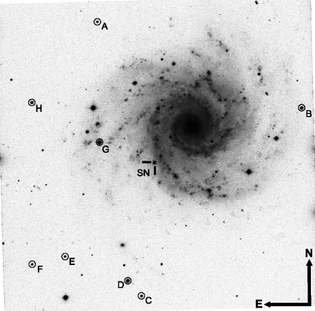
Figure 1.— SN 2013ej in NGC 0628. The $BR$-band composite image taken from 104-cm Sampurnanad telescope, covering an area of about 13′$\times$13′  is shown. Eight local field standards and SN are marked in the image.

Table 2Eight local standards in the field of SN 2013ej with corresponding coordinates ($\alpha,\delta$) calibrated magnitudes in UBVRI. Errors quoted here, include both photometric and calibration errors.

Star	$\alpha_{\rm J2000}$	$\delta_{\rm J2000}$	$U$	$B$	$V$	$R$	$I$
ID	(h m s)	(° ′ ″)	(mag)	(mag)	(mag)	(mag)	(mag)
A	1:36:57.9	+15:51:19.4	16.773 $\pm$ 0.0325	16.867 $\pm$ 0.0259	16.297 $\pm$ 0.0193	15.939 $\pm$ 0.0163	15.567 $\pm$ 0.0207
B	1:36:23.0	+15:47:45.3	15.102 $\pm$ 0.0289	15.109 $\pm$ 0.0302	14.580 $\pm$ 0.0234	14.253 $\pm$ 0.0183	13.888 $\pm$ 0.0260
C	1:36:50.4	+15:40:01.9	16.588 $\pm$ 0.0318	16.525 $\pm$ 0.0277	15.798 $\pm$ 0.0200	15.372 $\pm$ 0.0157	14.925 $\pm$ 0.0187
D	1:36:52.7	+15:40:39.4	14.811 $\pm$ 0.0318	14.561 $\pm$ 0.0265	13.817 $\pm$ 0.0184	13.384 $\pm$ 0.0167	12.976 $\pm$ 0.0196
E	1:37:03.4	+15:41:39.2	17.140 $\pm$ 0.0386	17.064 $\pm$ 0.0251	16.407 $\pm$ 0.0200	16.008 $\pm$ 0.0160	15.601 $\pm$ 0.0206
F	1:37:09.0	+15:41:20.4	18.804 $\pm$ 0.1537	17.800 $\pm$ 0.0282	16.769 $\pm$ 0.0249	16.146 $\pm$ 0.0167	15.583 $\pm$ 0.0205
G	1:36:57.6	+15:46:22.7	13.934 $\pm$ 0.0272	13.756 $\pm$ 0.0219	12.991 $\pm$ 0.0160	12.555 $\pm$ 0.0161	12.155 $\pm$ 0.0240
H	1:37:09.0	+15:48:00.6	16.974 $\pm$ 0.0434	16.172 $\pm$ 0.0249	15.175 $\pm$ 0.0157	14.598 $\pm$ 0.0170	14.062 $\pm$ 0.0194

Table 3Photometric evolution of SN 2013ej. Errors denote $1\sigma$ uncertainty.

UBVRI photometry
UT Date JD Phase^a $U$ $B$ $V$ $R$ $I$ Tel^b (yyyy-mm-dd) 2456000+ (day) (mag) (mag) (mag) (mag) (mag) 2013-08-04.82 509.32 12.02 12.026 $\pm$ 0.061 12.633 $\pm$ 0.020 12.612 $\pm$ 0.013 12.434 $\pm$ 0.017 12.349 $\pm$ 0.018 HCT 2013-08-31.93 536.43 39.13 14.576 $\pm$ 0.251 14.208 $\pm$ 0.020 13.125 $\pm$ 0.011 12.670 $\pm$ 0.015 12.436 $\pm$ 0.011 HCT 2013-09-29.77 565.27 67.97 16.088 $\pm$ 0.027 14.991 $\pm$ 0.020 13.569 $\pm$ 0.012 13.056 $\pm$ 0.016 12.750 $\pm$ 0.016 HCT 2013-09-30.72 566.22 68.92 16.207 $\pm$ 0.109 14.956 $\pm$ 0.020 13.595 $\pm$ 0.008 12.992 $\pm$ 0.015 12.741 $\pm$ 0.016 ST 2013-10-02.87 568.37 71.07 16.223 $\pm$ 0.028 15.017 $\pm$ 0.020 13.640 $\pm$ 0.012 13.053 $\pm$ 0.015 12.750 $\pm$ 0.017 HCT 2013-10-13.70 579.20 81.90 16.823 $\pm$ 0.054 15.291 $\pm$ 0.015 13.864 $\pm$ 0.010 13.222 $\pm$ 0.017 — ST 2013-10-15.85 581.35 84.05 17.026 $\pm$ 0.061 15.365 $\pm$ 0.021 13.884 $\pm$ 0.012 13.273 $\pm$ 0.011 12.978 $\pm$ 0.017 ST 2013-10-16.71 582.21 84.91 17.036 $\pm$ 0.089 15.406 $\pm$ 0.013 13.939 $\pm$ 0.010 13.288 $\pm$ 0.018 12.986 $\pm$ 0.025 ST 2013-10-21.73 587.23 89.93 17.292 $\pm$ 0.057 15.611 $\pm$ 0.017 14.126 $\pm$ 0.017 13.446 $\pm$ 0.016 13.147 $\pm$ 0.018 ST 2013-10-24.70 590.20 92.90 17.405 $\pm$ 0.035 15.743 $\pm$ 0.016 14.233 $\pm$ 0.021 13.540 $\pm$ 0.014 13.253 $\pm$ 0.014 ST 2013-10-25.72 591.22 93.92 17.365 $\pm$ 0.023 15.732 $\pm$ 0.014 14.340 $\pm$ 0.008 13.592 $\pm$ 0.011 13.322 $\pm$ 0.011 DFOT 2013-10-26.74 592.24 94.94 17.442 $\pm$ 0.020 15.795 $\pm$ 0.014 14.431 $\pm$ 0.007 13.672 $\pm$ 0.010 13.384 $\pm$ 0.011 DFOT 2013-10-27.76 593.26 95.96 17.515 $\pm$ 0.033 15.985 $\pm$ 0.022 14.453 $\pm$ 0.016 13.750 $\pm$ 0.016 13.447 $\pm$ 0.021 ST 2013-11-09.63 606.13 108.83 18.440 $\pm$ 0.039 17.611 $\pm$ 0.015 16.108 $\pm$ 0.012 15.144 $\pm$ 0.015 14.783 $\pm$ 0.016 HCT 2013-11-11.72 608.22 110.92 18.655 $\pm$ 0.106 17.725 $\pm$ 0.020 16.358 $\pm$ 0.012 15.357 $\pm$ 0.016 14.978 $\pm$ 0.016 ST 2013-11-12.67 609.17 111.87 — 17.700 $\pm$ 0.021 16.379 $\pm$ 0.014 15.358 $\pm$ 0.017 15.004 $\pm$ 0.014 ST 2013-11-14.65 611.15 113.85 — 17.764 $\pm$ 0.031 16.405 $\pm$ 0.011 15.402 $\pm$ 0.010 15.031 $\pm$ 0.013 ST 2013-11-19.69 616.19 118.89 18.515 $\pm$ 0.133 17.865 $\pm$ 0.023 16.493 $\pm$ 0.015 15.480 $\pm$ 0.016 15.133 $\pm$ 0.019 ST 2013-11-23.69 620.19 122.89 19.144 $\pm$ 0.408 17.945 $\pm$ 0.021 16.533 $\pm$ 0.009 15.529 $\pm$ 0.010 15.203 $\pm$ 0.011 ST 2013-11-24.62 621.12 123.82 18.973 $\pm$ 0.128 17.911 $\pm$ 0.019 16.552 $\pm$ 0.012 15.544 $\pm$ 0.015 15.205 $\pm$ 0.016 ST 2013-12-06.72 633.22 135.92 19.292 $\pm$ 0.171 18.113 $\pm$ 0.028 16.771 $\pm$ 0.014 15.719 $\pm$ 0.016 15.420 $\pm$ 0.017 ST 2013-12-08.73 635.23 137.93 19.286 $\pm$ 0.175 18.139 $\pm$ 0.018 16.815 $\pm$ 0.017 15.766 $\pm$ 0.022 15.486 $\pm$ 0.024 ST 2013-12-09.69 636.19 138.89 — 18.167 $\pm$ 0.022 16.832 $\pm$ 0.011 15.779 $\pm$ 0.017 15.488 $\pm$ 0.017 ST 2013-12-10.61 637.11 139.81 — 18.209 $\pm$ 0.034 16.863 $\pm$ 0.019 15.796 $\pm$ 0.020 15.490 $\pm$ 0.022 ST 2013-12-14.74 641.24 143.94 — 18.015 $\pm$ 0.093 16.892 $\pm$ 0.034 15.856 $\pm$ 0.020 15.597 $\pm$ 0.023 ST 2013-12-15.63 642.13 144.83 — 18.223 $\pm$ 0.041 16.974 $\pm$ 0.019 15.914 $\pm$ 0.025 15.603 $\pm$ 0.026 ST 2013-12-16.70 643.20 145.90 — 18.109 $\pm$ 0.053 16.943 $\pm$ 0.025 15.903 $\pm$ 0.019 15.596 $\pm$ 0.126 ST 2013-12-19.61 646.11 148.81 — 18.249 $\pm$ 0.043 17.009 $\pm$ 0.015 15.932 $\pm$ 0.019 15.661 $\pm$ 0.023 ST 2013-12-24.62 651.12 153.82 19.474 $\pm$ 0.061 18.265 $\pm$ 0.027 17.138 $\pm$ 0.014 16.003 $\pm$ 0.015 15.743 $\pm$ 0.016 ST 2013-12-25.66 652.16 154.86 — 18.321 $\pm$ 0.016 17.101 $\pm$ 0.010 16.012 $\pm$ 0.009 15.722 $\pm$ 0.012 ST,DFOT 2013-12-28.62 655.12 157.82 19.368 $\pm$ 0.058 18.325 $\pm$ 0.019 17.161 $\pm$ 0.009 16.041 $\pm$ 0.015 15.760 $\pm$ 0.016 DFOT 2013-12-29.59 656.09 158.79 19.436 $\pm$ 0.060 18.315 $\pm$ 0.024 17.180 $\pm$ 0.011 16.061 $\pm$ 0.010 15.791 $\pm$ 0.011 DFOT 2014-01-19.62 677.12 179.82 — 18.676 $\pm$ 0.025 17.458 $\pm$ 0.011 16.370 $\pm$ 0.014 16.128 $\pm$ 0.015 ST 2014-01-25.62 683.12 185.82 19.703 $\pm$ 0.071 18.638 $\pm$ 0.013 17.526 $\pm$ 0.009 16.424 $\pm$ 0.011 16.164 $\pm$ 0.012 DFOT 2014-01-30.62 688.12 190.82 19.797 $\pm$ 0.596 18.785 $\pm$ 0.027 17.602 $\pm$ 0.014 16.501 $\pm$ 0.013 16.282 $\pm$ 0.015 ST 2014-01-31.58 689.08 191.78 — 18.787 $\pm$ 0.030 17.618 $\pm$ 0.019 16.522 $\pm$ 0.017 16.273 $\pm$ 0.025 ST 2014-02-02.62 691.12 193.82 — 18.813 $\pm$ 0.035 17.623 $\pm$ 0.031 16.546 $\pm$ 0.020 16.323 $\pm$ 0.024 ST 2014-02-17.59 706.09 208.79 — 19.218 $\pm$ 0.079 17.814 $\pm$ 0.022 16.682 $\pm$ 0.012 16.470 $\pm$ 0.017 ST
Swift UVOT photometry
UT Date JD Phase^a $uvw2$ $uvm2$ $uvw1$ $uvu$ $uvb$ $uvv$ Tel^b (yyyy/mm/dd) 2456000+ (day) (mag) (mag) (mag) (mag) (mag) (mag) /Inst 2013-07-30.98 504.48 7.18 12.369 $\pm$ 0.040 12.023 $\pm$ 0.040 11.711 $\pm$ 0.039 — — 12.689 $\pm$ 0.042 Swift 2013-07-31.50 505.00 7.70 12.455 $\pm$ 0.040 12.097 $\pm$ 0.040 11.755 $\pm$ 0.039 — — 12.614 $\pm$ 0.040 Swift 2013-07-31.83 505.33 8.03 12.577 $\pm$ 0.035 12.204 $\pm$ 0.033 11.814 $\pm$ 0.032 — — — Swift 2013-08-03.06 507.56 10.26 13.044 $\pm$ 0.037 12.695 $\pm$ 0.041 — 11.675 $\pm$ 0.029 12.619 $\pm$ 0.029 — Swift 2013-08-03.18 507.68 10.38 13.056 $\pm$ 0.035 — — — 12.622 $\pm$ 0.029 — Swift 2013-08-04.85 509.35 12.05 13.374 $\pm$ 0.040 13.155 $\pm$ 0.053 — 11.812 $\pm$ 0.029 12.608 $\pm$ 0.029 — Swift 2013-08-04.98 509.48 12.18 13.385 $\pm$ 0.037 — — — — — Swift 2013-08-07.24 511.74 14.44 13.907 $\pm$ 0.041 — 12.948 $\pm$ 0.042 — — — Swift 2013-08-07.55 512.05 14.75 13.968 $\pm$ 0.050 — — — — — Swift 2013-08-08.02 512.52 15.22 14.039 $\pm$ 0.052 14.058 $\pm$ 0.070 13.131 $\pm$ 0.038 12.185 $\pm$ 0.031 12.749 $\pm$ 0.029 12.477 $\pm$ 0.030 Swift 2013-08-08.22 512.72 15.42 14.126 $\pm$ 0.045 — — 12.266 $\pm$ 0.029 — — Swift 2013-08-09.25 513.75 16.45 14.387 $\pm$ 0.055 14.305 $\pm$ 0.112 13.379 $\pm$ 0.041 12.333 $\pm$ 0.029 12.906 $\pm$ 0.029 12.535 $\pm$ 0.031 Swift 2013-08-09.31 513.81 16.51 — 14.406 $\pm$ 0.065 — — — — Swift 2013-08-11.78 516.28 18.98 15.210 $\pm$ 0.118 15.114 $\pm$ 0.109 13.907 $\pm$ 0.052 12.659 $\pm$ 0.029 12.983 $\pm$ 0.029 12.581 $\pm$ 0.031 Swift 2013-08-13.85 518.35 21.05 15.652 $\pm$ 0.082 15.964 $\pm$ 0.068 14.446 $\pm$ 0.059 12.982 $\pm$ 0.031 13.109 $\pm$ 0.029 12.599 $\pm$ 0.032 Swift 2013-08-15.00 520.50 23.20 16.209 $\pm$ 0.090 — 14.905 $\pm$ 0.069 13.308 $\pm$ 0.033 13.221 $\pm$ 0.030 12.573 $\pm$ 0.032 Swift 2013-08-17.65 522.15 24.85 16.588 $\pm$ 0.098 17.109 $\pm$ 0.195 15.201 $\pm$ 0.072 13.602 $\pm$ 0.035 13.293 $\pm$ 0.030 12.656 $\pm$ 0.032 Swift 2013-08-19.73 524.23 26.93 16.824 $\pm$ 0.105 17.554 $\pm$ 0.221 15.493 $\pm$ 0.076 13.964 $\pm$ 0.039 13.476 $\pm$ 0.030 12.692 $\pm$ 0.032 Swift 2013-08-22.54 527.04 29.74 17.245 $\pm$ 0.120 18.047 $\pm$ 0.250 15.890 $\pm$ 0.075 14.338 $\pm$ 0.045 13.663 $\pm$ 0.032 12.816 $\pm$ 0.033 Swift 2013-08-23.14 527.64 30.34 17.170 $\pm$ 0.117 — 15.866 $\pm$ 0.083 14.366 $\pm$ 0.045 13.627 $\pm$ 0.031 12.892 $\pm$ 0.034 Swift 2013-08-27.74 532.24 34.94 17.746 $\pm$ 0.146 18.569 $\pm$ 0.214 16.356 $\pm$ 0.095 14.844 $\pm$ 0.058 13.915 $\pm$ 0.033 12.965 $\pm$ 0.034 Swift 2013-09-06.16 541.66 44.36 18.133 $\pm$ 0.124 19.137 $\pm$ 0.190 16.793 $\pm$ 0.084 15.573 $\pm$ 0.067 — — Swift 2013-09-06.41 541.91 44.61 — — — 15.674 $\pm$ 0.087 14.367 $\pm$ 0.036 13.231 $\pm$ 0.035 Swift 2013-09-16.71 552.21 54.91 18.687 $\pm$ 0.158 19.486 $\pm$ 0.236 17.292 $\pm$ 0.096 16.229 $\pm$ 0.090 14.750 $\pm$ 0.039 13.470 $\pm$ 0.038 Swift 2013-09-26.45 561.95 64.65 18.793 $\pm$ 0.166 — 17.562 $\pm$ 0.123 16.585 $\pm$ 0.128 14.922 $\pm$ 0.042 13.604 $\pm$ 0.039 Swift 2013-10-06.88 572.38 75.08 19.241 $\pm$ 0.231 19.883 $\pm$ 0.333 17.919 $\pm$ 0.133 17.055 $\pm$ 0.094 — — Swift 2013-10-16.77 582.27 84.97 19.294 $\pm$ 0.247 — 18.127 $\pm$ 0.170 17.286 $\pm$ 0.164 15.464 $\pm$ 0.055 14.029 $\pm$ 0.045 Swift 2013-10-26.95 592.45 95.15 — — 18.248 $\pm$ 0.190 17.514 $\pm$ 0.171 — — Swift 2013-11-06.16 602.66 105.36 — — — 18.774 $\pm$ 0.304 — — Swift 2013-11-13.21 609.71 112.41 — — 19.523 $\pm$ 0.351 19.058 $\pm$ 0.306 — — Swift 2013-11-13.68 610.18 112.88 — — — 18.816 $\pm$ 0.263 17.974 $\pm$ 0.210 16.512 $\pm$ 0.148 Swift 2013-11-20.43 616.93 119.63 — — — 18.977 $\pm$ 0.214 17.889 $\pm$ 0.090 16.718 $\pm$ 0.080 Swift 2013-11-25.40 621.90 124.60 — — — 19.162 $\pm$ 0.323 — — Swift 2013-11-30.43 626.93 129.63 — — 19.726 $\pm$ 0.313 19.342 $\pm$ 0.280 18.155 $\pm$ 0.101 16.834 $\pm$ 0.082 Swift 2013-12-09.75 636.25 138.95 — — 19.807 $\pm$ 0.327 19.343 $\pm$ 0.274 18.196 $\pm$ 0.102 16.928 $\pm$ 0.085 Swift

^a with reference to the explosion epoch JD 2456497.30

^b ST : 104-cm Sampurnanand Telescope, ARIES, India; DFOT : 130-cm Devasthal fast optical telescope, ARIES, India; HCT: 2m Himalyan Chandra Telescope, Hanle, India; Swift: Swift UVOT

Note: Data observed within 5 Hrs, are represented under single epoch observation.

$$u = U+(7.800\pm 0.005)-(0.067\pm 0.009)\cdot(U-B)$$

$$b = B+(5.269\pm 0.007)-(0.060\pm 0.009)\cdot(B-V)$$

$$v = V+(4.677\pm 0.004)-(0.056\pm 0.005)\cdot(B-V)$$

$$r = R+(4.405\pm 0.005)-(0.038\pm 0.010)\cdot(V-R)$$

$$i = I+(4.821\pm 0.006)-(0.048\pm 0.006)\cdot(V-I)$$

where $u$, $b$, $v$, $r$ and $i$ are instrumental magnitudes corrected for time, aperture and airmass; $U$, $B$, $V$, $R$ and $I$ are standard magnitude. The standard-deviation of the difference between the calibrated and the standard magnitudes of the observed Landolt stars are found to be $\sim$ 0.03 mag in $U$, $\sim$ 0.02 mag in $BR$ and $\sim$ 0.01 mag in $VI$. The transformation coefficients were then used to generate eight local standard stars in the field of SN 2013ej, which are verified to be non-variable and have brightness similar to SN. These stars are identified in Fig.1 and the calibrated UBVRI magnitudes are listed in Table 2. These selected eight local standards were further used to standardize the instrumental light curve of the SN. One of these stars (star B) is common to that used in the study by Richmond (2014), and its BVRI magnitudes are found to lie within 0.03 mag of our calibrated magnitudes. Our calibrated magnitudes for SN 2013ej are also found to be consistent within errors to that presented in earlier studies of the event (Valenti et al., 2014; Richmond, 2014). The standard photometric magnitudes of SN 2013ej are listed in Table 3.

This supernova was also observed with the Ultra-Violet/Optical Telescope (UVOT; Roming et al., 2005) in six bands (viz. uvw2, uvm2, uvw1, uvu, uvb, uvv) on the Swift spacecraft (Gehrels et al., 2004). The UV photometry was obtained from the Swift Optical/Ultraviolet Supernova Archive (SOUSA; Brown et al., 2014). The reduction is based on that of Brown et al. (2009), including subtraction of the host galaxy count rates and uses the revised UV zeropoints and time-dependent sensitivity from Breeveld et al. (2011). The UVOT photometry is listed in Table. 3. The first month of UVOT photometry was previously presented by Valenti et al. (2014).

2.2. Spectroscopy

Spectroscopic observations have been carried out at 10 phases during 12 to 125d. Out of these, nine epochs of low resolution spectra are obtained from Himalaya Faint Object Spectrograph and Camera (HFOSC) mounted on 2.0m HCT. Spectroscopy on the HCT/HFOSC was done using a slit width of 1.92 arcsec, and grisms with resolution $\lambda/\Delta\lambda=1330$ for Gr7 and $2190$ for Gr8, and bandwidth coverage of $0.38-0.64$ $\mu m$ and $0.58-0.84$ $\mu m$ respectively. One high resolution spectrum is obtained from the ARC Echelle Spectrograph (ARCES) mounted on 3.5m ARC telescope located at Apache Point Observatory (APO). ARCES is a high resolution cross-dispersion echelle spectrograph, the spectrum is recorded in 107 echelle orders covering a wavelength range of $\lambda\sim$ 0.32-1.00$\mu{\rm m}$, at resolution of $R\sim 31500$ (Wang et al., 2003). Summary of spectroscopic observations is given in Table. 4.

Table 4Summary of spectroscopic observations of SN 2013ej. The spectral observations are made at 10 phases during 12d to 125d.

UT Date	JD	Phasea	Telescopec	Rangeb	Exposure
(yy/mm/dd.dd)	2456000+	(days)		$\mu{\rm m}$	(s)
2013-08-04.86	509.36	12.1	HCT	0.38-0.68	900
2013-08-27.76	532.26	35.0	HCT	0.38-0.68	1200
			HCT	0.58-0.84	1200
2013-09-03.90	539.40	42.1	HCT	0.38-0.68	1500
			HCT	0.58-0.84	1500
2013-09-29.78	565.28	68.0	HCT	0.38-0.68	1800
			HCT	0.58-0.84	2400
2013-10-02.89	568.39	71.1	HCT	0.38-0.68	1500
			HCT	0.58-0.84	1500
2013-10-11.28	576.78	79.5	APO	0.32-1.00	1200
2013-10-27.87	593.37	96.1	HCT	0.38-0.68	2400
2013-10-28.79	594.29	97.0	HCT	0.58-0.84	2400
2013-11-09.65	606.15	108.9	HCT	0.38-0.68	2100
			HCT	0.58-0.84	3900
2013-11-25.75	622.25	125.0	HCT	0.38-0.68	2400
			HCT	0.58-0.84	2400

^a With reference to the adopted explosion time JD 2456497.30

^b For transmission $\geq$50%

^c HCT : HFOSC on 2 m Himalyan Chandra Telescope, India; APO : Echelle spectrograph on 3.5 m ARC telescope at Apache Point Observatory, U.S.

^d At 0.6 $\mu{\rm m}$

Spectroscopic data reduction was done under the IRAF environment. Standard reduction procedures are followed for bias subtraction and flat fielding. Cosmic ray rejections are done using a Laplacian kernel detection algorithm for spectra, L.A.Cosmic (van Dokkum, 2001). One dimensional low resolution spectra were extracted using the apall task. Wavelength calibration was done using the identify task applied on FeNe and FeAr (for HCT) arc spectra taken during observation. Wavelength calibration was crosschecked against the [ O I ] $\lambda 5577$ sky line in the sky spectrum, and it was found to lie within 0.3 to 4.5 Å of the actual value. Spectra were flux calibrated using standard, sensfunc and calibrate tasks in IRAF. For flux calibration, spectrophotometric standards were used which were observed on the same nights as the SN spectra were recorded. All spectra were tied to absolute flux scale using the observed flux from UBVRI photometry of SN. To perform the tying, individual spectrum is multiplied by a wavelength dependent polynomial, which is convolved with UBVRI filters and then the polynomial is tuned to match the convolved flux with observations. The one dimensional calibrated spectra were corrected for heliocentric velocity of host galaxy (658 $\rm{\,km\,s^{-1}}$; Table 1) using dopcor task.

3. Distance and Extinction

We adopt a distance of $9.57\pm 0.70$ Mpc which is a mean value of four different distance estimation techniques used for NGC 0628, viz., 9.91 Mpc applying Standard Candle Method (scm) to SN 2003gd by Olivares et al. (2010); 10.19 Mpc using the Tully-Fisher method (HyperLeda); 9.59 Mpc using brightest supergiant distance estimate by Hendry et al. (2005); and planetary nebula luminosity function distance 8.59 Mpc (Herrmann et al., 2008). Although for each of these methods number of distance estimates exists in literature, we tried to select only most recent estimates. Richmond (2014) estimated a distance of $9.1\pm 0.4$ Mpc by applying Expanding Photosphere Method (EPM) to SN 2013ej, which we find consistent to that we adopted.

One of the most reliable and well accepted method for SNe line-of-sight reddening estimation is using the Na i  D absorption feature. The equivalent width (EW) of Na i  D doublet ($\lambda\lambda$ 5890, 5896) is found to be correlated with the reddening, estimated from the tail color curves of type Ia SNe (Barbon et al., 1990; Turatto et al., 2003). However, Poznanski et al. (2011) suggested that although Na i  D EW is weakly correlated with $E(B-V)$, the EWs estimated from low resolution spectra is a bad estimator of $E(B-V)$. Poznanski et al. (2012) used a larger sample of data and presented a more precise and rather different functional form of the correlation than that was derived earlier. Our high resolution echelle spectra at 79.5d provided an excellent opportunity to investigate the line-of-sight extinction.

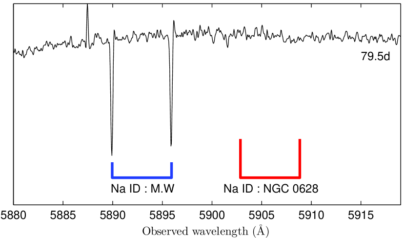
Figure 2.— Echelle spectra at 79.5d showing the Na i  D doublet for Milky-way while no impression for NGC 0628 is detected.

The resolved Na i  D doublet for Milky-way is clearly visible in the high-resolution spectra (recorded on 79.5d) as shown in Fig.2. Whereas no impression of Na i  D for NGC 0628 is detected at the expected redshifted position relative to Milky-way. This indicates that the reddening due to host is negligible, only Galactic reddening will contribute to the total line of sight extinction. A similar conclusion has also been inferred by Valenti et al. (2014) from their high resolution spectra obtained at 31d. Thus, we adopt a total $\mbox{$E(B-V)$}=0.060\pm 0.001$ mag, which is entirely due to Galactic reddening (Schlafly & Finkbeiner, 2011) and assuming total-to-selective extinction at V band as $R_{V}=3.1$, it translates into $A_{V}=0.185\pm 0.004$ mag.

4. Light curve

4.1. Light curve evolution and comparison

The optical light curves of SN 2013ej in UBVRI and six UVOT bands are shown in Fig. 3. UBVRI photometric observations were done at 38 phases during 12 to 209d (from plateau to nebular phase). The duration of plateau phase is sparsely covered, while denser follow-up initiated after 68d. The plateau phase lasted until $\sim 85$d with an average decline rate of 6.60, 3.57, 1.74, 1.07 and 0.74 mag (100 d)^-1 in UBVRI bands respectively. Since 95d, the light curve declines very fast until 115d, after which it settles to a relatively slow declining nebular phase. During this phase the decline rates for UBVRI bands are 0.98, 1.22, 1.53, 1.42 and 1.55 mag (100 d)^-1 respectively.

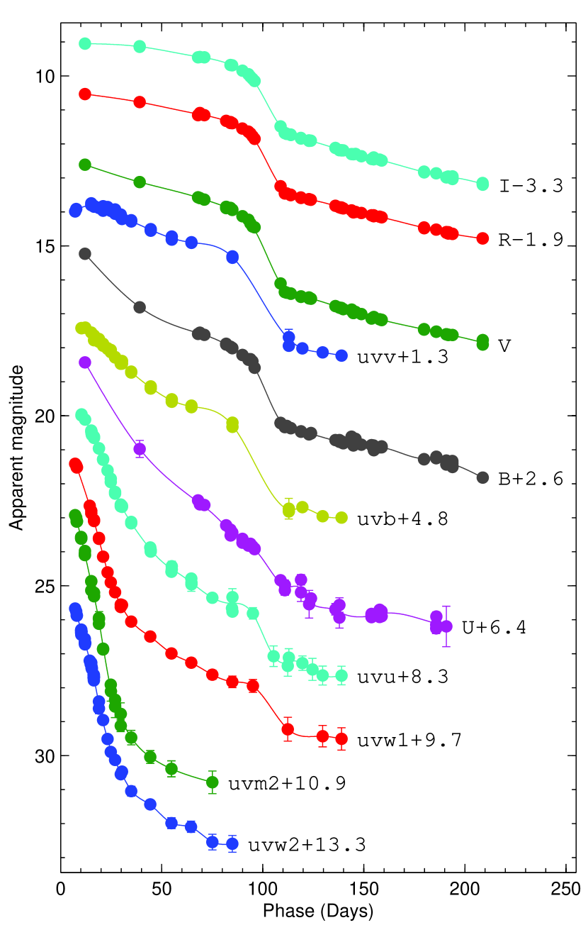
Figure 3.— The photometric light curves in Johnson-Cousins UBVRI and Swift UVOT bands. The light curves are vertically shifted for clarity. The line joining the data points of light curves is for visualization purpose only.

SN 2013ej has been also observed by Swift UVOT at 35 phases during 7 to 139d. The UVOT UV band light curves declines steeply during the first 30d at a rate of 0.182, 0.213, 0.262 mag d^-1 in uvw1, uvw2 and uvm2 bands respectively, thereafter settling into a slow declining phase until it reaches the end of plateau.

SN 2013ej experience a steeper plateau decline than that observed for SN 1999em (Leonard et al., 2002c), SN 1999gi (Leonard et al., 2002b), SN 2012aw (Bose et al., 2013) and SN 2013ab (Bose et al., 2015). For example, SN 2012aw plateau declines at a rate of 5.60, 1.74, 0.55 mag (100 d)^-1 in $UBV$-bands, similarly for SN 2013ab decline rates in UBVRI are 7.60, 2.72, 0.92, 0.59 and 0.30 mag (100 d)^-1 and 0.169, 0.236, 0.257 mag d^-1 in UVOT uvw1, uvw2 and uvm2 bands (during first 30d).

The absolute V-band ($M_{V}$) light curve of SN 2013ej is plotted in Fig. 4 and is compared with other well studied type II SNe (after correcting for extinction and distance). In Table 5 we list the plateau slope of all compared type II events. The comparison shows that the decline rate of SN 2013ej during this phase is highest (1.74 mag (100 d)^-1) among most other SNe, except three type IIL SNe 1980K, 2000dc and 2013by, where SN 1980 is among the very first observed prototypical type IIL event. The early plateau ($<40$d) light curve of SN 2013ej is identical to SN 2009bw. However, unlike most other IIP SNe, e.g. 2009bw and 2013ab, which becomes flatter during late plateau, SN 2013ej continues to decline almost at a steady rate until the end of plateau ($\sim$ 85d). The mid-plateau $M_{V}=-14.7$ mag for SN 2013ej, which places it in the class of normal luminous type II events. SN 2013ej is comparable with fast declining and short plateau SNe in the sample of Anderson et al. (2014b). Following the plateau phase, $V$-band light drops very fast to reach slow declining nebular phase (1.53 mag (100 d)^-1), which is powered by the radioactive decay of ⁵⁶Co to ⁵⁶Fe. The fall of $M_{V}$ during the plateau nebular transition is $\sim 2.4$ mag, which is on the higher side of the compared events. The closest comparison is SNe 2009bw and 2012A which exhibits a drop of $\sim$2.4 mag and $\sim$2.5 mag respectively. This also indicates low amount of ⁵⁶Ni mass synthesized during the explosion which we shall further discuss in the next section.

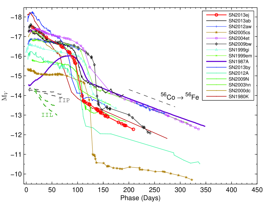
Figure 4.— The M_V light curve of SN 2013ej is compared with other type II SNe. The exponential decline of the tail light curve following the radioactive decay law for ⁵⁶Co$\rightarrow$⁵⁶Fe is shown with a dashed line. On the bottom left side, pair of dotted lines in each gray and green colors represent the slope range for type IIP and IIL SNe templates as given by Faran et al. (2014). The adopted explosion time in JD-2400000, distance in Mpc, $E(B-V)$ in mag and the reference for observed V-band magnitude, respectively, are : SN 1980K – 44540.5, 5.5, 0.30; Barbon et al. (1982), NED database; SN 1987A – 46849.8, 0.05, 0.16; Hamuy & Suntzeff (1990); SN 1999em – 51475.6, 11.7, 0.10; Leonard et al. (2002a); Elmhamdi et al. (2003); SN 1999gi – 51522.3, 13.0, 0.21; Leonard et al. (2002b); SN 2000dc – 51762.4, 49.0, 0.07; Faran et al. (2014), NED database; SN 2003hn – 52866.5, 17.0, 0.19; Krisciunas et al. (2009); Anderson et al. (2014b); SN 2004et – 53270.5, 5.4, 0.41; Sahu et al. (2006); SN 2005cs – 53549.0, 7.8, 0.11; Pastorello et al. (2009); SN 2009N – 54848.1, 21.6, 0.13; Takáts et al. (2014); SN 2009bw – 54916.5, 20.2, 0.31; Inserra et al. (2012); SN 2012A – 55933.5, 9.8, 0.04; Tomasella et al. (2013); SN 2012aw – 56002.6, 9.9, 0.07; Bose et al. (2013); SN 2013ab – 56340.0, 24.0, 0.04; Bose et al. (2015); SN 2013by – 56404.0, 14.8, 0.19; Valenti et al. (2015).

Table 5Parameters estimated from V band light cruve

SN Name	Plateau slopea	Transition dropb	Transition timec
	mag (100 d)-1	mag	days
SN1980K	3.63 $\pm$ 0.04	2.0$\pm$0.04	37 $\pm$ 5
SN2000dc	2.56 $\pm$ 0.06i	–	–
SN2013by	2.01 $\pm$ 0.02	2.2$\pm$0.03	19 $\pm$ 5
SN 2013ej	1.74 $\pm$ 0.08	2.4$\pm$0.02	21 $\pm$ 3
SN2003hn	1.41 $\pm$ 0.04	2.0$\pm$0.04	19 $\pm$ 4
SN2012A	1.12 $\pm$ 0.03	2.5$\pm$0.02	23 $\pm$ 4
SN2009bw	0.93 $\pm$ 0.04	2.4$\pm$0.03	14 $\pm$ 3
SN2004et	0.73 $\pm$ 0.02	2.1$\pm$0.04	27 $\pm$ 6
SN2013ab	0.54 $\pm$ 0.02	1.7$\pm$0.02	25 $\pm$ 2
SN2012aw	0.51 $\pm$ 0.02	–	–
SN1999gi	0.47 $\pm$ 0.02	2.0$\pm$0.02	29 $\pm$ 3
SN2005cs	0.44 $\pm$ 0.03	4.0$\pm$0.03	24 $\pm$ 3
SN2009N	0.36 $\pm$ 0.03	2.0$\pm$0.04	26 $\pm$ 3
SN1999em	0.31 $\pm$ 0.02	1.9$\pm$0.02	28 $\pm$ 4

Note: Objects are sorted in order of plateau slope.

^a Plateau slope during the linear decline phase, starting after first minima until plateau end.

^b Drop in magnitude during the plateau to nebular transition.

^c Duration of plateau to nebular transition.

ⁱ Slope is calculated up to the available range of data, as plateau end is not observed.

Swift UVOT absolute magnitude light curves of SN 2013ej are shown in Fig. 5 and compared with other well observed type II SNe. The sample is selected in such a way that SNe have at least a month of observations. Most SNe are not followed for more than a month by Swift, mainly because of the large distances or high extinction values. However, both these factors work in favor of SN 2013ej  making it possible to have about four months of observations. Moreover, the location of the SN being in the outskirt of a spiral arm of NGC 0628, the background flux contamination is also negligible. The comparison shows that the SN 2013ej UV light curves are identical to SN 2012aw. SN 2013ej also shows a similar UV plateau trend as observed in SN 2012aw (Bayless et al., 2013), which is although expected but rarely detected for IIP/L SNe.

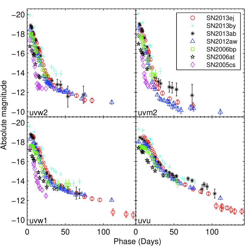
Figure 5.— Comparison of the Swift UVOT UV absolute light curves of SN 2013ej, with other well observed II SNe from UVOT. For the compared SNe, references for UVOT data, extinction and distance are: SN 2005cs – Brown et al. (2009); Pastorello et al. (2009), SN 2006at – Brown et al. (2009); Distance 65 Mpc; $\mbox{$E(B-V)$}=0.031$ mag (only Galactic reddening Schlafly & Finkbeiner, 2011), SN 2006bp – Dessart et al. (2008), SN 2012aw – Bayless et al. (2013); Bose et al. (2013), SN 2013ab – Bose et al. (2015), SN 2013by – Brown et al. (2014); Valenti et al. (2015). Some late data points for SN 2013ab with large errors has been omitted from the plot.

Broadband color provides important information to study the temporal evolution of SN envelope. In Fig. 6, we plot the intrinsic colors U-B, B-V, V-R and V-I for SN 2013ej and compare its evolution with type II-pec SN 1987A, and type IIP SNe 1999em, 2004et, 2012aw and 2013ab. All the colors show generic signature of fast cooling ejecta until the end of plateau ($\sim 110$d). With the start of the nebular phase it continues to cool at a much slower rate in V-I and V-R colors, whereas U-V and B-V shows a bluer trend. This is because, as the SN enters the nebular phase, the ejecta become depleted of free electrons, thereby making the envelope optically thin, and so unable to thermalize the photons from radioactive decay of ⁵⁶Co to ⁵⁶Fe.

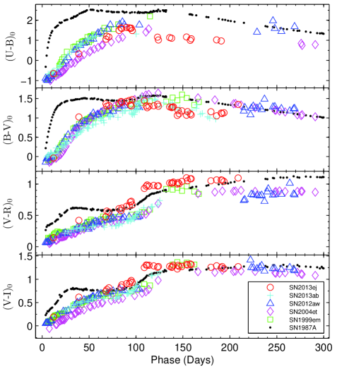
Figure 6.— The intrinsic colors evolution of SN 2013ej is compared with other well-studied type IIP SNe 1987A, 1999em, 2004et, 2012aw and 2013ab. The reference for the data is same as in Fig. 4.

4.2. Bolometric light-curve

We compute the pseudo-bolometric luminosities following the method described in Bose et al. (2013); which include SED integration over the semi-deconvolved photometric fluxes after correcting for extinction and distance. Supernova bolometric luminosities during early phases ($\leq 30$d) are dominated by ultraviolet fluxes, while after mid-plateau ($\sim 50$d) UV contribution becomes insignificant as compared to optical counterpart (e.g., as seen in SNe 2012aw, 2013ab; Bose et al., 2013, 2015). Similarly, during late phases $>100$d NIR becomes dominant over optical fluxes. However, during most of the light curve evolution, optical fluxes still provide significant contribution. We compute pseudo-bolometric luminosities in the wavelength range of U to I band (3335-8750Å). We also computed UV-optical pseudo-bolometric light curve with wavelength starting from uvw2 band (wavelength range of 1606-8750Å). The UV contribution enhances the luminosity significantly during early phases, whereas it is almost negligible after mid-plateau.

In Fig. 7, we plot pseudo bolometric light curve for SN 2013ej and compare it with other SNe light curves computed using the same technique. We also include UV-optical bolometric light curve for SNe 2012aw and 2013ab along with SN 2013ej for comparison. Although the UV-optical light curve is initially brighter than the optical light curve, they completely coincide by the end of plateau phase (85d). It is evident from the comparison that SN 2013ej experienced a steep decline during the plateau phase, but with a much shorter duration. This is consistent with the anti-correlation observed between plateau slope and duration for type II SNe (Blinnikov & Bartunov, 1993; Anderson et al., 2014b). The UV-optical bolometric light decreases by 0.83 dex during plateau phase (from 12 to 85d), followed by an even faster drop by 0.76 dex in a short duration of 21 days (from 90 to 111d). Thereafter, the SN settles in a slow declining nebular phase. The tail luminosities are significantly lower than other normal luminosity IIP events, e.g., SN 2013ej luminosities are lower by $\sim 0.5$ dex (at 200d) than that of type II SNe 1987A, 1999em, 2004et and 2012aw, but higher than subluminous events like SN 2005cs. Another noticeable dissimilarity of the tail light curve is its high decline rate. SN 2013ej tail luminosity declines at a rate of 0.55 dex 100 d^-1, which is much higher than that expected from radioactive decay of ⁵⁶Co to ⁵⁶Fe. This is possibly because of inefficient gamma-ray trapping in the ejecta, and thus incomplete thermalization of the photons. We shall further explore this in §7 in context of modeling the light curve.

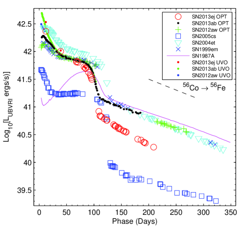
Figure 7.— The UBVRI bolometric light-curve of SN 2013ej is compared with other well studied supernovae. Light curves with added UVOT UV contributions are also shown for SNe 2013ej, 2013ab and 2012aw (labeled as UVO). The adopted values of distances, reddening and explosion time are same as in Fig. 4. The exponential decline of the tail light curve following the radioactive decay law is shown with a dashed line.

4.3. Mass of nickel

During the explosive nucleosynthesis of silicon and oxygen, at the time of shock-breakout in CCSNe, radioactive ⁵⁶Ni is produced. The nebular-phase light-curve is mainly powered by the radioactive decay of ⁵⁶Ni to ⁵⁶Co and ⁵⁶Co to ⁵⁶Fe with half-life times of 6.1d and 77.1d respectively emitting $\gamma$-rays and positrons. Thus the tail luminosity will be proportional to the amount of radioactive ⁵⁶Ni synthesized at the time of explosion. We determine the mass of ⁵⁶Ni using following two methods.

For SN 1987A, one of the most well studied and well observed event, the mass of ⁵⁶Ni produced in the explosion has been estimated quite accurately, to be $0.075\pm 0.005$ M_⊙ (Arnett, 1996). By comparing the tail luminosities of SN 2013ej and SN 1987A at similar phases, it is possible to estimate the ⁵⁶Ni mass for SN 2013ej. In principle true bolometric luminosities (including UV, optical and IR) are to be used for this purpose, which are available for SN 1987A, whereas for SN 2013ej we have only UV and optical observations. Thus, in order to have uniformity in comparison, we used only the UBVRI bolometric luminosities for both SNe and computed using the same method and wavelength range. We estimate the tail UBVRI luminosity at 175d, by making a linear fit over 155 to 195d, to be $2.90\pm 0.43\times 10^{40}$ erg s^-1. Likewise, SN 1987A luminosity is estimated to be $9.60\pm 0.06\times 10^{40}$ erg s^-1 at similar phase. Thus, the ratio of SN 2013ej to SN 1987A luminosity is $0.302\pm 0.044$, which corresponds to a ⁵⁶Ni mass of $0.023\pm 0.003\mbox{M${}_{\odot}$}$ for SN 2013ej.

Assuming the $\gamma$-photons emitted from radioactive decay of ⁵⁶Co thermalize the ejecta, ⁵⁶Ni mass can be independently estimated from the tail luminosity as described by Hamuy (2003).

$$M_{\rm Ni}=7.866\times 10^{-44}\times L_{t}\exp\left[\frac{(t_{t}-t_{0})/(1+z)-6.1}{111.26}\right]\mbox{M${}_{\odot}$}$$

where $t_{0}$ is the explosion time, 6.1d is the half-life time of ⁵⁶Ni and 111.26d is the e-folding time of the ⁵⁶Co decay. We compute tail luminosity $L_{t}$ at 6 epochs within 153 to 185d from the $V$ band data corrected for distance, extinction and bolometric correction factor of $0.26\pm 0.06$ mag during nebular phase (Hamuy, 2003). The weighted mean value of $L_{\rm t}$ is found to be $5.45\pm 0.35\times 10^{40}\,$$\rm{\,erg\,s^{-1}}$corresponding to mean phase of 170d. This tail luminosity corresponds to a value of $M_{\rm Ni}=0.019\pm 0.002$M_⊙.

We take the weighted mean of the estimated values from above two methods, and adopt a ⁵⁶Ni mass of $0.020\pm 0.002\mbox{M${}_{\odot}$}$ for SN 2013ej.

Hamuy (2003) found a strong correlation between the ⁵⁶Ni mass and the mid plateau (at 50d) $V$ band absolute magnitude for type II SNe and this correlation was further confirmed by Spiro et al. (2014) specifically for low luminous events. Fig. 8 shows the correlation of mid plateau M_V versus ⁵⁶Ni mass for 34 events, including SN 2013ej. The SN lies within the scatter relation, but towards the lower mass range of ⁵⁶Ni than where most of the events cluster around (top right).

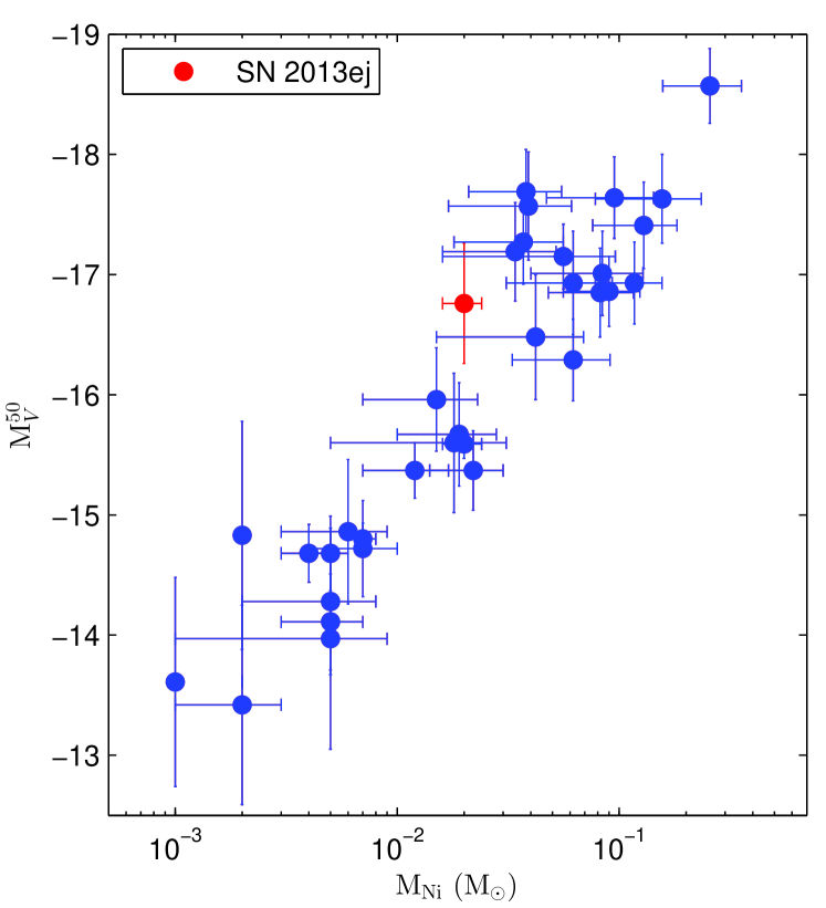
Figure 8.— The plot of absolute $V$ band magnitude at 50 day versus ⁵⁶Ni mass for 34 type II SNe. Data taken from Hamuy (2003) and Spiro et al. (2014). The position of SN 2013ej on the correlation is shown with filled red circle.

5. Optical spectra

5.1. Key spectral features

The spectroscopic evolution of SN 2013ej is presented in Fig. 9. Preliminary identifications of spectral features has been done as per previously studied type IIP SNe (e.g., Leonard et al., 2002a; Bose et al., 2013). The spectrum at 12d shows broad H$\alpha$, H$\beta$ and He i  features on top of a hot blue continuum. The 35d spectrum shows a relatively flat continuum with well developed features of H$\alpha$, H$\beta$, Fe ii  along with blends of other heavier species Ti ii  and Ba ii . He i  line is no longer detectable, instead Na i  D features start to appear at similar location. The spectra from 35 to 80d represent the cooler photospheric phase, where the photosphere starts to penetrate deeper layers rich in heavier elements like Fe ii  and Sc ii . During these phases we see the emergence and development of various other heavy atomic lines and their blends like Ti ii , Ba ii , Na i  D and Ca ii . Fig. 10 shows the comparison of three plateau phase spectra, viz. 12, 35 and 68d with other well studied type IIP SNe at similar epochs. The comparison shows the spectra of SN 2013ej is broadly identical to others in terms of observable line features and their evolution. A notable feature during early spectrum (12d) is the dip on the bluer wing of H$\alpha$ profiles near 6170 Å  which can be attributed as the Si ii  feature. Leonard et al. (2013) also identified this feature at $\sim 9$d spectra of SN 2013ej  however, due to unlikeliness of such a strong Si ii  feature at such early epochs, a possiblity of non-standard red supergiant envelope or CSM interaction was suggested. However, such dips are detectable in 35 and 42d spectra, which we identify as Si ii  feature in synow modeling.

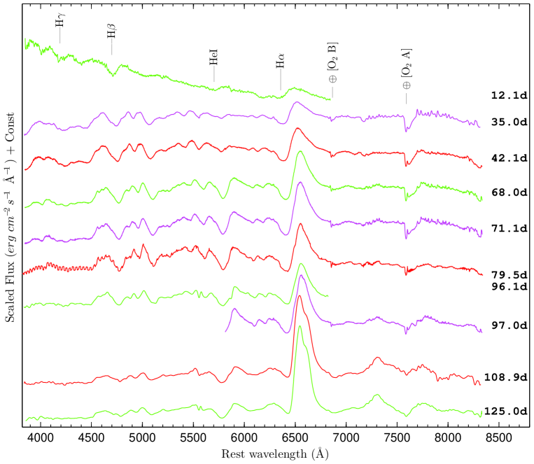
Figure 9.— The redshift corrected spectra of SN 2013ej are plotted for 10 phases during 12d to 125d. The prominent P-Cygni profiles of hydrogen (H$\alpha$, H$\beta$, H$\gamma$) and helium ( He i  $\lambda$5876) are marked. The telluric absorption features of O₂ are marked with $\oplus$, symbol. Portion of spectra in extreme blue or red ends have low SNR. Individual spectra with with overall low SNR has been binned for better visualization.

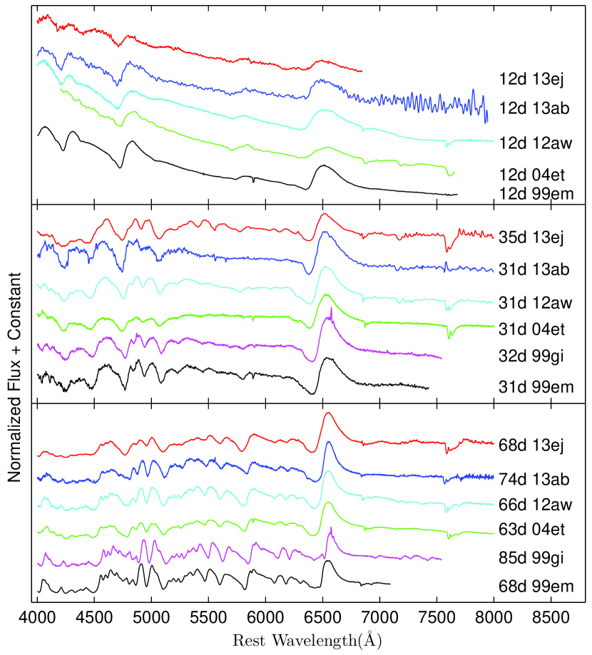
Figure 10.— Comparison of early (12d) and plateau (35d, 68d) phase spectra of SN 2013ej with other well-studied type IIP SNe 1999em (Leonard et al., 2002a), 1999gi (Leonard et al., 2002b), 2004et (Sahu et al., 2006; Maguire et al., 2010), 2012aw (Bose et al., 2013) and 2013ab (Bose et al., 2015). All comparison spectra are corrected for extinction and redshift (adopted values are same as in Fig. 4).

The spectra at 96 and 97d represents the plateau-nebular transition phase. Thereafter, spectra at 109 and 125d represents the nebular phase, where the ejecta has become optically thin. These spectra shows the emergence of some emission features from forbidden lines of [ O i ] $\lambda\lambda$ 6300, 6364 and [ Ca ii ] $\lambda\lambda$ 7291, 7324Å, as well as previously evolved permitted lines of H i , and the Na i  $\lambda$5893 doublet (see Fig. 11).

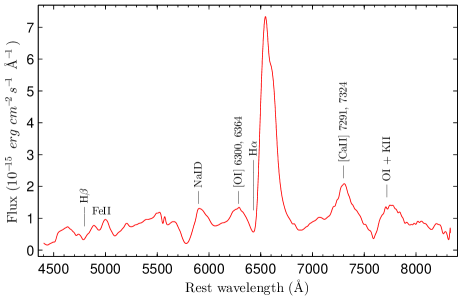
Figure 11.— The nebular phase spectrum of SN 2013ej at 125d. Prominent emission and absorption features are marked and labeled.

Gutiérrez et al. (2014) found correlations between H$\alpha$ absorption to emission strengths and light curve parameters, i.e. plateau slope and duration of optically thick phase. Following their selection criteria for choosing phase of SN spectra, i.e. ten days after start of recombination, we selected 42d spectrum as the closet available phase to the criteria. The H$\alpha$ absorption to emission ratio of equivalent widths for SN 2013ej is found to be $0.23\pm 0.02$, the optically thick phase is $\sim 85$d and B-band late plateau (40 to 85d) slope is $\sim 0.27$ mag (100 d)^-1. The correlation for optically thick phase duration is found to follow that presented by Gutiérrez et al. (2014). For the plateau slope, the correlation also hold true, but here SN 2013ej lies in the border line position of the scattered relation. However, it may be noted that H$\alpha$ profiles are possibly contaminated by high velocity features as we describe in next sections, which may result in deviation from correlation.

5.2. SYNOW modelling of spectra

SN 2013ej spectra has been modeled with synow (Fisher et al., 1997, 1999; Branch et al., 2002) for line identification and its velocity estimation. synow is a highly parametrized spectrum synthesis code which employs the Sobolev approximation to simplify radiation transfer equations assuming a spherically symmetric supernova expanding homologously. The strength of the synow code is its capability to reproduce P-Cygni profiles simultaneously in synthetic spectra for a given set of atomic species and ionization states. The applicability of synow is well tested in various core-collapse SNe studies (e.g. Inserra et al., 2012; Bose et al., 2013; Milisavljevic et al., 2013; Bose & Kumar, 2014; Takáts et al., 2014; Marion et al., 2014) for velocity estimation and analysis of spectral lines.

To model the spectra we tried various optical depth profiles (viz. gaussian, exponential and power law) with no significant difference among them, however we find exponential profile ($\tau\propto exp[-v/v_{e}]$) marginally better suited to match the absorption trough of observed spectra, where $v_{e}$ the e-folding velocity, is a fitted parameter. While modeling spectra, H i  lines are always dealt as detached scenario. This implies the velocity of hydrogen layer is significantly higher and is thus detached from photospheric layer, close to which most heavier atomic lines form, as assumed in synow code. As a consequence to this, the H$\alpha$ lines in synthetic spectrum, which are highly detached, has flat topped emissions with blue shifted absorption counter parts.

SN 2013ej spectra are dereddened and approximate blackbody temperature is supplied in the model to match the spectral continuum. For early spectrum (12d), local thermodynamic equilibrium (LTE) assumption holds good and thus synow could fit the continuum well, whereas at later epochs it fails to fit properly. The set of atomic species incorporated to generate the synthetic model spectrum are H i , He i ; Fe ii ; Ti ii ; Sc ii ; Ca ii ; Ba ii ; Na i  and Si ii . The photospheric velocity $v_{\rm ph}$ is optimized to simultaneously fit the Fe ii  ($\lambda\lambda$ 4924, 5018, 5169) P-Cygni profiles and H i  lines are treated as detached. The optical depths and optical depth profile parameters, e-folding velocity are varied for individual species to fit respective line profiles. In Fig. 12 we show the model fit of 71d spectrum. Most of the observable spectral features are reproduced well and are identified in the figure.

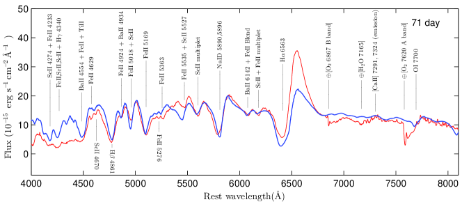
Figure 12.— synow modelling of SN 2013ej spectrum at 71d. Model spectrum is shown with thick solid line (blue), while the observed one is shown with thin solid line (red). Observed fluxes are corrected for extinction.

Similarly all spectra during 12 to 97d are modeled with synow. The model fits for Fe ii  ($\lambda\lambda$ 4924, 5018, 5169), H$\beta$ and H$\alpha$ spectral sections are shown in Fig. 13. The atomic species which are important to model these features are H i , Fe ii , Ba ii , Ti ii , Sc ii  and Na i . In addition to these Si ii  is also used to model the dips in the blue wing of H$\alpha$ P-Cygni during 12 to 42d. While modeling the H$\alpha$ and H$\beta$ profiles, synow was unable to properly fit the broad and extended P-Cygni absorption troughs with single regular component. In order to fit these extended troughs, we invoke high-velocity (HV) component of H i . Although no separate dip is seen, possibly due to low spectral resolution and overlapping of broad P-Cygni profiles, the HV component can well reproduce the observed features in synthetic model spectrum. The implication and interpretation of these HV components are further discussed in §5.4. The synow-derived velocities for Fe ii , H$\alpha$, H$\beta$ lines and corresponding HV components are listed in Table 6. The nebular spectra during 109 to 125d have not been modeled primarily due to limitations of the LTE assumption of synow, and also because nebular phase spectra are dominated by emission lines rather than P-Cygni profiles.

Table 6The line velocities of H$\alpha$, H$\beta$, Fe ii  ($\lambda\lambda$ 4924, 5018, 5169) and He i  $\lambda$5876 as estimated by modelling the observed spectra of SN 2013ej with synow. Fe ii  or He i  lines velocities are taken to represent photospheric velocity ($v_{\rm phm}$).

UT Date	Phasea	$v$( He i )	$v$( Fe ii )	$v$(Hα)	$v$(Hα) HVb	$v$(Hβ)	$v$(Hβ) HVb
(yyyy-mm-dd)	(day)	$10^{3}$ $\rm{\,km\,s^{-1}}$	$10^{3}$$\rm{\,km\,s^{-1}}$	$10^{3}$$\rm{\,km\,s^{-1}}$	$10^{3}$$\rm{\,km\,s^{-1}}$	$10^{3}$$\rm{\,km\,s^{-1}}$	$10^{3}$$\rm{\,km\,s^{-1}}$
2013-08-04.86	12.1	8.8	–	9.6	–	9.7	–
2013-08-27.76	35.0	–	6.7	7.9	–	6.6	–
2013-09-03.90	42.1	–	5.8	7.2	8.5	5.4	6.4
2013-09-29.78	68.0	–	3.6	5.8	7.4	4.0	5.8
2013-10-02.89	71.1	–	3.3	5.4	7.3	3.8	5.8
2013-10-11.28	79.5	–	3.3	5.2	6.3	3.6	4.8
2013-10-27.87	96.1	–	2.7	4.9	6.3	3.5	4.8
2013-10-28.79	97.0	–	2.7	4.8	6.3	–	–

^a With reference to the time of explosion JD 2456497.30

^b High velocity component used to fit the broad H$\alpha$ and H$\beta$ profile.

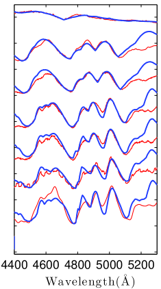
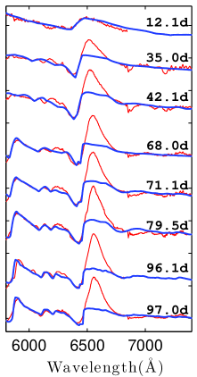
Figure 13.— synow modelling of SN 2013ej spectra at 8 phases during 12d to 97d for H$\beta$, Fe ii  multiplet (left) and H$\alpha$ (right) profiles. Model spectra are shown with thick solid line (blue), while the observed ones are shown with thin solid line (red). In the model, H i  lines are treated as detached to fit the absorption troughs. Along with Fe ii  and H i ; other ions ( Sc ii , Ba ii , Si ii and Na i , Ti ii ) are also incorporated in model to fit some weaker features, specially at later phases. In addition to this, high-velocity H i  lines are also incorporated (42d onwards) to fit the extended H$\alpha$ and H$\beta$ absorption troughs. The 97d spectrum do not have H$\beta$ and Fe ii  wavelength region, hence it is not shown here.

5.3. Evolution of spectral lines

Investigation of the spectral evolution sheds light on various important aspects of the SN, like interaction of ejecta with the circumstellar material, geometrical distribution of expanding shell of ejecta and formation of dust during late time. SN spectra are dominated by P-Cygni profiles which are direct indicators of expansion velocities and they evolve with the velocity of photosphere. As ejecta expands and opacity decreases allowing photons to escape from deeper layers rich in heavier elements, we are able to see emergence and growth of various spectral lines.

To illustrate the evolution of H$\alpha$ line, in Fig. 14 partial region of spectra is plotted in velocity domain corresponding to rest wavelengths of H$\alpha$. At 12d broad P-Cygni profile (FWHM $\sim 9500$ $\rm{\,km\,s^{-1}}$) is visible which becomes narrower with time as the expansion slows down. The blue-shifted absorption troughs are direct estimator of expansion velocity of the associated line forming layer. The emission peaks are found to be blue-shifted (by $\sim 3200$ $\rm{\,km\,s^{-1}}$at 12d), which progressively decreases with decrease in expansion velocity and almost settling to zero velocity when the SN starts to enter nebular phase (97d). Such blue-shifted emission peaks, especially during early phases are generic features observable in SN spectra, e.g., SNe 1987A (Hanuschik & Dachs, 1987), 1998A (Pastorello et al., 2005), 1999em (Elmhamdi et al., 2003), 2004et (Sahu et al., 2006), 2012aw (Bose et al., 2013), 2013ab (Bose et al., 2015). These features are tied with the density structure of the ejecta, which in turn controls the amount of occultation of the receding part of ejecta, resulting in biasing of the emission peak (Anderson et al., 2014a), which are not limited to H$\alpha$ but applicable to all spectral lines. However, such a blue-shift is clearly detected for H$\alpha$  whereas for most other lines, emission profiles are weak and peaks are contaminated by adjacent P-Cygni profiles. Detailed SN spectral synthesis code like cmfgen (Dessart & Hillier, 2005b) is capable of reproducing such blue-shifted emission peaks.

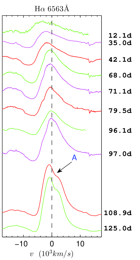
Figure 14.— Evolution of H$\alpha$ line profile at 10 phases during 12d to 125d. A zero-velocity line is plotted with a dashed line corresponding to the rest wavelength of H$\alpha$ $\lambda$6563.

As inferred from Fig. 10, the spectral evolution of SN 2013ej is almost identical to other typical IIP SNe. However, the comparison of 35 and 68d spectra indicates Fe ii  lines are somewhat under developed as compared to other SNe at similar phase. As seen in the 68d comparison, the Fe ii  ($\lambda\lambda$ 4924, 5018, 5169) absorption dips are significantly weaker in comparison to that seen in other SNe.

Another prominent and unusual feature is seen in nebular spectra at 109d and 125d, on top of H$\alpha$ emission, and the same is marked as feature A in Fig. 14. This unusual dip is resulting into an apparent blue-shift of the emission peak, which is in fact larger than that seen in the last plateau spectra at 97d. Such evolution is unexpected and against the general trend of emission peak evolution in SNe. The low resolution of these spectra prohibits us from investigating this feature in detail. This feature can be split into two emission components, one redshifted at 1200 $\rm{\,km\,s^{-1}}$ and another blueshifted by 1300 $\rm{\,km\,s^{-1}}$ (see §A for further explanation) with respect to H$\alpha$ rest position. Such an asymmetric or double peaked H$\alpha$ nebular emission has been observed in a number of SNe, e.g. SN 1999em (Leonard et al., 2002a) and SN 2004dj (Chugai et al., 2005). Leonard et al. (2002a) identified such a dip or notch in H$\alpha$ emission profile only during nebular phase of SN 1999em, which they suggested as possible ejecta-CSM interaction or asymmetry in line emitting region. In SN 2004dj, the asymmetry in nebular H$\alpha$ spectra identified by Chugai et al. (2005) has been explained by bipolar distribution of ⁵⁶Ni with a spherical hydrogen envelope (Chugai, 2006).

5.4. Ejecta velocity

Progenitor stars prior to explosion develop stratified layers of different elements, which are generally arranged in an elemental sequence, hydrogen being abundant in the outermost shell, whereas heavier metals like iron predominate at deeper layers. However at the time of shock breakout significant mixing of layers may occur. Spectral lines originating from different layers of the ejecta attains different characteristic velocities. Thus study of velocity evolution provides important clues to the explosion geometry and the characteristics of various layers. Evolution of photospheric layer is of special interest as it is directly connected to the kinematics and other related properties. Photosphere represents the layer of SN atmosphere where optical depth attains a value of $\sim~{}^{2}/_{3}$ (Dessart & Hillier, 2005a). Due to complex mixing of layers and continuous recession of the recombination front, no single spectral line can represent the true photospheric layer. During the plateau phase, Fe ii  or Sc ii  lines are the best estimator of photospheric velocity ($v_{\rm ph}$). In early phases when Fe ii  lines are not strongly detectable, the best proxy for $v_{\rm ph}$ is He i , or H$\beta$ (Takáts & Vinkó, 2012) in even earlier phases.

Line velocities can either be estimated by directly locating the P-Cygni absorption troughs, as done using splot task of IRAF, or by by modeling the line profiles with velocity as one of the input, as we do in synow. In Fig. 15, we plot the line velocities of H$\alpha$, H$\beta$, Fe ii  ($\lambda\lambda$ 4924, 5018, 5169) and Sc ii  ($\lambda\lambda$ 4670, 6247), using the absorption minima method. It is evident that Fe ii  and Sc ii  line velocities are very close to each other and they are formed at deeper layers, whereas H$\alpha$ and H$\beta$ line velocities are consistently higher at all phases as they form at larger radii. The synow estimated photospheric velocities are also plotted for comparison, which is very close to the Fe ii  and Sc ii  velocities estimated from absorption minima method. Here the synow-derived photospheric velocities are estimated by modelling He i  line for 12d spectrum and Fe ii  lines for rest of the spectra. Velocities for various lines estimated using synow are tabulated in Table 6.

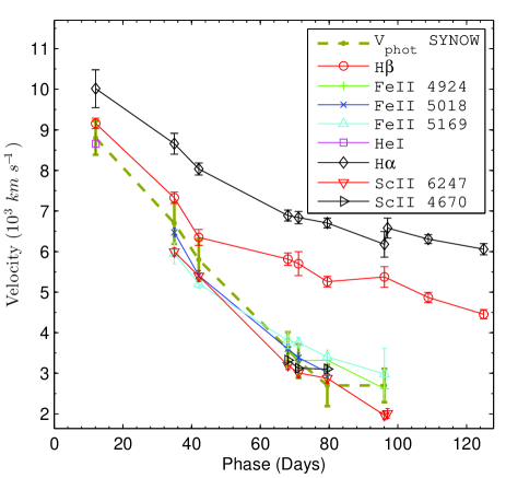
Figure 15.— Velocity evolution of H$\alpha$, H$\beta$, He i , Sc ii  and Fe ii  lines. The velocities are estimated using blueshift of the absorption minima. The expansion velocity of photosphere ($v_{\rm phm}$) estimated from synow modeling of He i  line at 12d and Fe ii  lines at later phases (see Table 6) are also overplotted for comparison.

Fig. 17 shows the comparison of photospheric velocity of SN 2013ej with other well-studied type II SNe 1987A, 1999em, 1999gi, 2004et, 2005cs, 2012aw and 2013ab. For the purpose of comparison the absorption trough velocities have been used, taking the mean of Fe ii  line triplet, or He i  lines at early phases where Fe ii  lines are not detectable. The velocity profile of SN 2013ej is very similar to other normal IIP SNe 1999em, 1999gi, 2004et, 2012aw and 2013ab, on the other hand velocities of SN 2005cs and 1987A are significantly lower. The velocity profile of SN 2013ej  is almost identical with SNe 2004et, 2012aw and 2013ab, whereas it is consistently higher than SNe 1999gi and 1999em by $\sim 800-900$$\rm{\,km\,s^{-1}}$. For comparison of H i  (H$\alpha$ and H$\beta$) velocities, we have chosen all those events which are at least photometrically and spectroscopically similar to SN 2013ej. Comparison reveals that, H velocities during later phases (60-100 d) are consistently higher than all comparable events. SNe 2012aw and 2013ab, have photospheric velocities identical to SN 2013ej, but their H velocities are significantly lower by large values, e.g., for SN 2013ej the H$\alpha$ velocity at 80d is higher by 1500 $\rm{\,km\,s^{-1}}$ and H$\beta$ is higher by 2400 $\rm{\,km\,s^{-1}}$. Likewise, H velocities for SNe 1999em and 1999gi are even lower at similar phases. Although SN 2004et H i  velocities are somewhat on higher end, they are still significantly less than those of SN 2013ej. It is also to be noted that, at 12d SN 2013ej  H i  velocities are consistent and similar to those of other normal SNe, but as it evolves these velocities decline relatively slowly, ultimately turning out into a higher velocity profile after $\sim 40$d.

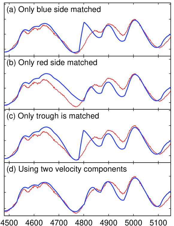
Figure 16.— For 68d spectrum, the H$\beta$ profile is fitted using synow with various velocity components. (a) The fit only with a single high velocity component to match the blue wing of the absorption dip, (b) with a single low velocity component to match the red wing, (c) with single velocity to only fit the trough, (d) with two velocity components to fit entire absorption profile.

5.5. High velocity components of H i  and CSM interaction

As discussed in §5.2, the broad and extended H$\alpha$ or H$\beta$ absorption profiles are not properly reproduced using single H i  velocity component in synow, and those profiles can only be fitted by incorporating a high-velocity (HV) components along with the regular one. Fig. 16 shows the comparison of synow fits for 68d H$\beta$ profile with various single velocity as well as for combined two velocity components. A single velocity component at 5600 $\rm{\,km\,s^{-1}}$ can match the blue wing well and partially the trough, whereas, it does not match the red side at all. Similarly, with a single velocity component at 4000 $\rm{\,km\,s^{-1}}$  can partially match the red slope of the trough, but does not include the trough as well as the extended blue wing. By only matching the trough position, the model fits for a single velocity of 5300 $\rm{\,km\,s^{-1}}$, which does not fit either of the blue or red wing. Even-though the ‘detachment’ of H i  from photosphere in synow model makes the fit of red wing worse by steepening it further, but it is still conclusive that none of these single velocity component can properly reproduce the absorption profile. It is only by including two velocity components together in the model could reproduce the entire H$\beta$ profile. Such a scenario start to appear from 42d spectrum which only becomes stronger as the line evolves until 97d. The H$\alpha$ troughs are also reproduced in a similar fashion. However, it may be noted, that such an extended H i  feature may also be explained as a possible outcome of a different (complex and extended) density profile which synow can not reproduce.

The comparison of H$\alpha$ and H$\beta$ velocities with other normal IIP SNe (see Fig. 17), estimated by directly locating the P-Cygni absorption troughs, shows that SN 2013ej velocities are significantly higher and declines relatively slowly (especially during later phases; 60-100d) as compared to those seen in typical IIP SNe, e.g., 1999em, 1999gi, 2012aw or 2013ab. On the other hand the photospheric velocity comparison with other IIP SNe does not show any such anomaly. This, we suggest as the effect of blending with H i  HV components in H$\alpha$ and H$\beta$, which we could separate out while modeling these broad features with synow having two velocity components. The regular H$\alpha$ and H$\beta$ velocities estimated from synow declines at a normal rate consistent to that seen in other SNe (see Fig.17), whereas the HV components remains at higher velocities by $1000-2000$ $\rm{\,km\,s^{-1}}$, declining at relatively slower rate. It is also interesting to note that the velocity difference between the regular and HV component for H$\alpha$ and H$\beta$ is similar at same epochs. Chugai et al. (2007) identified similar HV absorption features associated close to H$\alpha$ and H$\beta$ troughs in SNe 1999em and 2004dj, which remained constant with time. Presence of such HV features has also been detected in SN 2009bw (Inserra et al., 2012) and SN 2012aw (Bose et al., 2013) which is suggestive of interaction of SN ejecta with pre-existent CSM. Similar to SN 2013ej, HV signatures has been detected all throughout the plateau phase evolution of SN 2009bw, while in SN 2012aw such features were only detected at late plateau phase (55 to 104d). Although, we found HV components in SN 2013ej by modeling the extended P-Cygni troughs, we are unable to visually detect such two individual velocity components, this is possibly because of our signal-to-noise-ratio limited spectra and weaker strength of HV components. Chugai et al. (2007) argued that SN ejecta can interact with the cooler dense shell of CMS material, which might have originated from the pre-supernova mass loss in the form of stellar winds. Their analysis showed that such interaction can led to the detection of HV absorption features on bluer wings of Balmer lines due to enhanced excitation of the outer layers of unshocked ejecta. We, therefore suggest weak or moderate ejecta-CSM interaction in SN 2013ej. X-ray emission from SN 2013ej has also been reported by Margutti et al. (2013), which they measured a 0.3-10 keV count-rate of 2.7$\pm$0.5 cps, translating into a flux of $\sim 1.1\times 10^{-13}$ erg s^-1cm^-2 (assuming simple power-law spectral model with photon index Gamma $=2$). Such X-ray emission may also indicate ejecta-CSM interaction suffered by SN 2013ej.

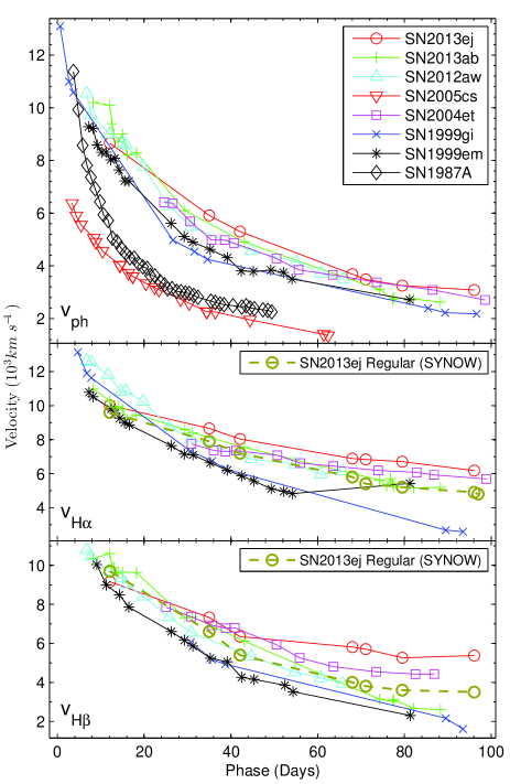
Figure 17.— The photospheric velocity (top) evolution ($v_{\rm ph}$) of SN 2013ej is compared with other well-studied type II SNe. The $v_{\rm ph}$ plotted here are the absorption trough velocities (average of Fe ii  lines at late phases and He i  at early phases). Similar comparison of P-Cygni absorption velocities, but for H$\alpha$ and H$\beta$ are shown in middle and bottom panels respectively. The regular velocity component for H$\alpha$ and H$\beta$ estimated from synow (without HV components; see Table. 6) are also plotted for comparison.

6. Status of SN 2013ej in type II diversity

6.1. Factors favoring SN 2013ej as type IIL

Having characterized the event both photometrically and spectroscopically, we may now revisit the aspects which favor SN 2013ej as type IIL event. The SN was originally classified as type IIP (Valenti et al., 2013) based on spectroscopic similarity to SN 1999gi. Due to same underlying physical mechanisms which govern both type IIP and IIL SNe, early spectra may not clearly distinguish these sub classes of SN type II. The distinguishing factor among IIP and IIL is nominal and mainly depend upon light curve characteristics. SN 2013ej shows a decline of 1.74 mag (100 d)^-1 (see Table 5) or $\sim 0.87$ mag in 50 days, which definitely falls in the criteria of type IIL SNe as proposed by Faran et al. (2014). In Fig. 4, the spread of template light curves for type IIP and IIL (Faran et al., 2014) is shown along with M_V light curves of SNe sample. It is evident that under this scheme of classification, SN 2013ej is not a type IIP, rather it is marginally within the range of type IIL template light curves. This is also justified from the point of basic idea behind these classifications, that type IIP must show a ‘plateau’ of almost constant brightness for some time ($\sim 90$d), which is not the case with SN 2013ej. Due to the very fact that SN type II light curves and physical properties exhibit a continuum distribution rather than a bi-modality (Anderson et al., 2014b), SN 2013ej shows intermediate characteristic in the SN type II diversity.

One distinguishing spectroscopic property Faran et al. (2014) found for type IIL SNe is the overall higher photospheric ( Fe ii  $\lambda$5196) velocity and flatter H i  (H$\beta$ and H$\alpha$) velocity profiles as compared to type IIP counterpart. Although Fe ii  velocities are on the higher end as compared to typical IIP SNe velocities, we do not find it as a remarkable deviation to distinguish SN 2013ej from IIP sample. However, we do see a anomaly in H$\alpha$, H$\beta$ absorption minima velocity profiles, as they start off with velocities consistent with those of type IIP but declines relatively slowly (see §5.4 for more description of this feature) ultimately surpassing faster declining IIP velocity profiles after 50 days. This characteristic feature of H i  velocities for SN 2013ej is typical for most IIL SNe as found by Faran et al. (2014).

6.2. CSM interaction and type IIL

Faran et al. (2014) proposed a possible explanation for the flatter velocity profiles in IIL SNe, which is due the lack of hydrogen in deeper and slow expanding layers of ejecta, resulting into higher H i  absorption velocities arising mostly from outer layer. However, for SN 2013ej we suggest the flattening of H$\alpha$ and H$\beta$ velocity profiles are due to the contamination of HV component of H i  (see §5.5). Indication of CSM interaction in SN 2013ej may also be inferred from X-ray detection by Margutti et al. (2013). Valenti et al. (2015) found SN 2013by, a type IIL SN, to be moderately interacting with CSM. This led them to ask the prevalence of CSM interaction among IIL SNe in general. Type IIL SNe originate from progenitors similar to IIPs, but have lost a significant fraction of hydrogen before explosion during pre SN evolution. Hence it may not be usual to detect HV H i  signatures in H$\alpha$, H$\beta$ absorption profiles as a consequence of ejecta-CSM interaction. A moderate or weak interaction may produce a HV component blending with H$\alpha$, H$\beta$ profiles, which may result into shift in absorption minima, rather than a prominent secondary HV dip. Such a scenario may perfectly explain the relatively higher and flatter H i  velocity profiles of most type IIL SNe as compared to IIP counterparts, found by Faran et al. (2014) based on direct velocity estimates of absorption minima.

Another example of CSM interaction in type IIL is SN 2008fq, which does show strong interaction signature like a type IIn (Taddia et al., 2013), but also shows a steep decline like IIL during first 60 days (Faran et al., 2014). Supernova PTF11iqb (Smith et al., 2015) is also a type IIn SN, having prominent CSM interaction signatures, but with IIL like steeper light curve. Initial spectra of this SN showed IIn characteristics, however late plateau spectra revealed features similar to type IIL. PTF11iqb originated from a progenitor identical to type IIP/L, instead of a LBV as expected for a typical IIn. However, because of rare detection of type IIL events and its fast decline in magnitudes we do not have sufficient information to investigate CSM interaction in all such objects. Thus, the question still remains open if all or most IIL SNe interact with CSM and whether the flatter H i  absorption minima velocity profiles is a consequence of interaction.

7. Light curve modelling

To determine the explosion parameters of SN 2013ej, the observed light curve is modeled following the semi-analytical approach originally developed by Arnett (1980) and further refined in Arnett & Fu (1989). More appropriate and accurate approach would have been detailed hydrodynamical modeling (e.g. Falk & Arnett, 1977; Utrobin, 2007; Bersten et al., 2011; Pumo & Zampieri, 2011) to determine explosion properties, however application of simple semi-analytical models (Arnett, 1980, 1982; Arnett & Fu, 1989; Popov, 1993; Zampieri et al., 2003; Chatzopoulos et al., 2012) can be useful to get preliminary yet reliable estimates of the parameters without running resource intensive and time consuming hydrodynamical codes. Nagy et al. (2014) also followed the original semi-analytical formulation presented by Arnett & Fu (1989) and modeled a few well studied II SNe. The results are compared with hydrodynamical models from the literature and are found to be in good agreement. The model light-curve is computed by solving the energy balance of the spherically symmetric supernova envelope, which is assumed to be in homologous expansion having spatially uniform density profile.

The temperature evolution is given as (Arnett, 1980),

$$T(x,t)^{4}=T_{0}^{4}\psi(x)\phi(t)\left(\frac{R_{0}}{R(t)}\right)^{4},$$

where $x$ is defined as dimensionless co-moving radius relative to the mass of the envelope and, $\psi(x)$ is the radial component of temperature profile which falls off with radius as $sin(\pi x)/\pi x$. Here we incorporate the effect of recombination, as shock heated and ionized envelope expands and cools down to recombine at temperature $T_{rec}$. We define $x_{i}$ as the co-moving radius of the recombination front and the opacity ($\kappa$) changes very sharply at this layer such that $\kappa\approx 0$ for the ejecta above $x_{i}$. Following the treatment of Arnett & Fu (1989) the temporal component of temperature, $\phi(t)$ can be expressed as (Nagy et al., 2014),

$$\frac{d\phi(t)}{dz}=\frac{R(t)}{R_{0}x_{i}^{3}}\left[p_{1}\zeta(t)-p_{2}\phi(t)x_{i}-2x_{i}^{2}\phi(t)\frac{R_{0}}{R(t)}\frac{dx_{i}}{dz}\right],$$

here $\zeta(t)$ is the total radioactive energy input from decay chain of unit mass of ⁵⁶Ni, which is normalized to the energy production rate of ⁵⁶Ni. The rest of the parameters in the equation have usual meaning and can be found in aforementioned papers. From this ordinary differential equation we can find out the solution of $\phi(t)$ using Runge-Kutta method. The treatment adopted to determine $x_{i}$ is somewhat similar to Nagy et al. (2014), where we numerically determine the radius $x_{i}$ (to an accuracy of $10^{-12}$) for which the temperature of the layer reaches $T_{rec}$. Once we find out the solution of $\phi(t)$ and $x_{i}$, the total bolometric luminosity is calculated as the sum of radioactive heating and rate of energy released due to recombination,

$$L(t)=x_{i}\frac{\phi(t)E_{th}(0)}{\tau_{d}}\left(1-e^{-A_{g}/t^{2}}\right)+4\pi r_{i}^{2}Q\rho(x_{i},t)R(t)\frac{dx_{i}}{dt},$$

here, $d(x_{i})/dt$ is the inward velocity of co-moving recombination front and the term $[1-exp(-A_{g}/t^{2})]$, takes into account of gamma-ray leakage from the ejecta. The factor $A_{g}$ is the effectiveness of gamma ray trapping (see e.g., Clocchiatti & Wheeler, 1997; Chatzopoulos et al., 2012), where large $A_{g}$ means full trapping of gamma rays, this factor is particularly important to model the SN 2013ej tail light curve. In this relation we also modified the second term to correctly account for the amount of envelope mass being recombined.

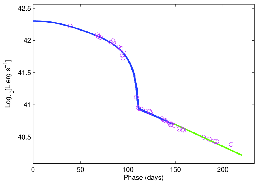
Figure 18.— Model fit (solid line) on the observed bolometric light curve (open circles) of SN 2013ej. The green solid line follows only the radioactive decay law, where the recombination front has completely disappeared.

To model SN light curves it is essential to obtain the true bolometric luminosity from observations. Since our data is limited only to optical and UV bands, we adopt the prescription for color dependent bolometric corrections by Bersten & Hamuy (2009) to obtain bolometric light curve for SN 2013ej. Figure 18 shows the model fit with the observed bolometric light curve of the SN. We estimate an ejecta mass of 12 M_⊙, progenitor radius of 450 R_⊙ and explosion energy (kinetic + thermal) of 2.3 foe ($10^{51}$ erg). The uncertainty in mass and radius is about 25%. We find that the plateau duration is strongly correlated with explosion energies (especially kinetic), and also with $\kappa$ and $T_{rec}$. Thus depending upon these parameters our model is consistent with a wide range of explosion energies, with 2.3 foe towards the lower end and energies up to 4.5 foe at higher end. Assuming the mass of the compact remnant to be 1.5-2.0 M_⊙, the total progenitor mass adds up to be 14M_⊙.

The mass of radioactive ⁵⁶Ni estimated from the model is 0.018M_⊙, which primarily governs the tail light curve of the SN. As discussed in §4.2, the slope of the tail light curve observed for SN 2013ej is significantly higher than other typical IIP SNe and also to that expected from radioactive decay of ⁵⁶Co to ⁵⁶Fe. The light curve powered by full gamma-ray trapping from radioactive decay chain of $\mbox{${}^{56}$Ni}\rightarrow\mbox{${}^{56}$Co}\rightarrow\mbox{${}^{56}$Fe}$ results in a slower decline and does not explain the steeper tail observed in SN 2013ej. In the model we decreased the gamma-ray trapping effectiveness parameter $A_{g}$ to $3\times 10^{4}$ day², which matches the steeper radioactive tail. The gamma-ray optical depth can be related to this parameter as $\tau_{g}\sim A_{g}/t^{2}$. This implies that the gamma-ray leakage in SN 2013ej is significantly higher than other typical type IIP SNe.

Valenti et al. (2014) using early temperatures ($<5$ days) of SN 2013ej provided a preliminary estimate of the progenitor radius as $400-600$ R_⊙, which is in good agreement with our result. Our progenitor mass estimate is also consistent with that reported by Fraser et al. (2014) from direct observational identification of the progenitor using HST archival images, which is $8-15.5$ M_⊙.

8. Summary

We present photometric and spectroscopic observations of SN 2013ej. Despite low cadence optical photometric follow up during photospheric phase, we are able to cover most of the important phases and features of light curve.

Our high resolution spectrum at 80d shows the presence of Na i  D ($\lambda\lambda$ 5890, 5896) doublet for Milky Way, while no impression for host galaxy NGC 0628. This indicates that SN 2013ej suffers minimal or no reddening due to its host galaxy.

The optical light curves are similar to type IIL SNe, with a relatively short plateau duration of 85d and steeper decline rates of 6.60, 3.57, 1.74, 1.07 and 0.74 mag 100 day^-1 in UBVRI bands respectively. The comparison of absolute V band light curves shows that SN 2013ej suffers the higher decline rate than all type IIP SNe, but similar to type IIL SNe 1980k, 2000dc and 2013by. The drop in luminosity during the plateau-nebular transition is also higher than most type II SNe in our sample, which is 2.4 mag in V band.

The UVOT UV optical light curves shows steep decline during first 30 days at a rate of 0.182, 0.213, 0.262 mag d^-1 in uvw1, uvw2 and uvm2 bands respectively. The absolute UV light curves are identical to SN 2012aw and also shows a similar UV-plateau trend as observed in SN 2012aw.

Owing to the large drop in luminosity during plateau-nebular transition, the light curve settles to a significantly low luminous tail phase as compared to other normal IIP SNe. The mass of radioactive ⁵⁶Ni estimated from the tail bolometric luminosity is $0.020\pm 0.002$ M_⊙, which is in between normal IIP SNe (e.g., 1999em, 2004et, 2012aw) and subluminous events, like SN 2005cs.

The spectroscopic features and their evolution is similar to normal type II events. Detailed synow modelling has been performed to identify spectral features and to estimate velocities for H$\alpha$, H$\beta$, Fe ii  ($\lambda\lambda$ 4924, 5018, 5169) and Sc ii  ($\lambda\lambda$ 4670, 6247) lines. The photospheric velocity profile of SN 2013ej, which is represented by Fe ii  lines and He i  line at 12d, is almost identical to SNe 2004et, 2012aw and 2013ab. The H$\alpha$, H$\beta$ velocities estimated by directly locating the absorption troughs are significantly higher and slow declining as compared to other normal IIP events. However, such H i  velocity profiles are typical for type IIL SNe.

The P-Cygni absorption troughs of H$\alpha$ and H$\beta$ are found to be broad and extended which a single H i  component in synow model could not fit properly. However, these extended features are fitted well with synow by incorporating a high velocity H i  component. These HV components can be traced throughout the photospheric phase which may indicate possible ejecta-CSM interaction. Our inference is also supported by the detection of X-ray emission from the SN 2013ej (Margutti et al., 2013) indicating possible CSM interaction, and the unusually high polarization reported by Leonard et al. (2013) may also further indicate asymmetry in environment or ejecta of the SN. Such CSM interaction and their signature in H$\alpha$, H$\beta$ profiles has also been reported for SNe 2009bw (Inserra et al., 2012) and 2012aw (Bose et al., 2013).

Nebular phase spectra during 109 to 125d phases are dominated by characteristic emission lines, however the H$\alpha$ line shows an unusual notch, which may be explained by superposition of HV emission on regular H$\alpha$ profile. Although, the origin of the feature is not fully explained, it may indicate bipolar distribution of ⁵⁶Ni in the core.

We modeled the bolometric light curve of SN 2013ej and estimated a progenitor mass of $\sim 14$M_⊙, radius of $\sim 450$R_⊙ and explosion energy of $\sim 2.3$ foe. These progenitor property estimates are consistent to those given by Fraser et al. (2014) and Valenti et al. (2014) for mass and radius respectively. The tail bolometric light curve of SN 2013ej, is found to be significantly steeper than that expected from decay chain of radioactive ⁵⁶Ni. Thus, in the model we decreased the effectiveness of gamma ray trapping, which could explain the steeper slope of tail light curve.

Appendix A Nebular H$\alpha$ profile

The unusual notch in nebular H$\alpha$ profile can be described as a superimposition of two profiles. Fig. 19 shows the observed H$\alpha$ profile at 125d which is fitted by two component Gaussian profiles. These two profiles are separated by 55 Å ($\sim 2500$ $\rm{\,km\,s^{-1}}$), one being blue shifted by -1300 $\rm{\,km\,s^{-1}}$ while the other is red shifted at 1200 $\rm{\,km\,s^{-1}}$ with respect to rest H$\alpha$ position. The FWHM for the blue component is 54Å and for red component is 146Å. The redshifted component is dominant in strength over the blue one, having their ratio of equivalent widths to be 4.5. It may be noted that for the sake of simplicity and only for the purpose of illustration we used Gaussian profiles, which does not account for the P-Cygni absorption troughs as we see on bluer wings of line profiles in observed SN spectrum.

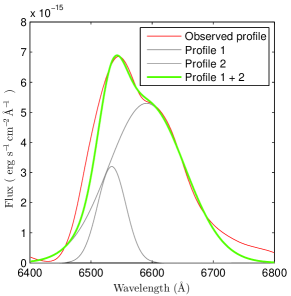
Figure 19.— H$\alpha$ profile of 125d spectrum fitted by two component gausian profile seperated by $\sim$2500 $\rm{\,km\,s^{-1}}$.

References

- Anderson et al. (2014a) Anderson, J. P., et al. 2014a, MNRAS, 441, 671
- Anderson et al. (2014b) Anderson, J. P., et al. 2014b, ApJ, 786, 67
- Arcavi et al. (2012) Arcavi, I., et al. 2012, ApJL, 756, L30
- Arnett (1996) Arnett, D. 1996, Supernovae and Nucleosynthesis: An Investigation of the History of Matter from the Big Bang to the Present
- Arnett (1980) Arnett, W. D. 1980, ApJ, 237, 541
- Arnett (1982) Arnett, W. D. 1982, ApJ, 253, 785
- Arnett & Fu (1989) Arnett, W. D., & Fu, A. 1989, ApJ, 340, 396
- Barbon et al. (1990) Barbon, R., Benetti, S., Rosino, L., Cappellaro, E., & Turatto, M. 1990, A&A, 237, 79
- Barbon et al. (1979) Barbon, R., Ciatti, F., & Rosino, L. 1979, A&A, 72, 287
- Barbon et al. (1982) Barbon, R., Ciatti, F., & Rosino, L. 1982, A&A, 116, 35
- Bayless et al. (2013) Bayless, A. J., et al. 2013, ApJL, 764, L13
- Bersten et al. (2011) Bersten, M. C., Benvenuto, O., & Hamuy, M. 2011, ApJ, 729, 61
- Bersten & Hamuy (2009) Bersten, M. C., & Hamuy, M. 2009, ApJ, 701, 200
- Blinnikov & Bartunov (1993) Blinnikov, S. I., & Bartunov, O. S. 1993, A&A, 273, 106
- Bose & Kumar (2014) Bose, S., & Kumar, B. 2014, ApJ, 782, 98
- Bose et al. (2013) Bose, S., et al. 2013, MNRAS, 433, 1871
- Bose et al. (2015) Bose, S., et al. 2015, ArXiv e-prints
- Branch et al. (2002) Branch, D., et al. 2002, ApJ, 566, 1005
- Breeveld et al. (2011) Breeveld, A. A., Landsman, W., Holland, S. T., Roming, P., Kuin, N. P. M., & Page, M. J. 2011, in American Institute of Physics Conference Series, Vol. 1358, American Institute of Physics Conference Series, ed. J. E. McEnery, J. L. Racusin, & N. Gehrels, 373
- Brown et al. (2014) Brown, P. J., Breeveld, A. A., Holland, S., Kuin, P., & Pritchard, T. 2014, Ap&SS, 354, 89
- Brown et al. (2009) Brown, P. J., et al. 2009, AJ, 137, 4517
- Burrows (2013) Burrows, A. 2013, Reviews of Modern Physics, 85, 245
- Chatzopoulos et al. (2012) Chatzopoulos, E., Wheeler, J. C., & Vinko, J. 2012, ApJ, 746, 121
- Chugai (2006) Chugai, N. N. 2006, Astronomy Letters, 32, 739
- Chugai et al. (2007) Chugai, N. N., Chevalier, R. A., & Utrobin, V. P. 2007, ApJ, 662, 1136
- Chugai et al. (2005) Chugai, N. N., Fabrika, S. N., Sholukhova, O. N., Goranskij, V. P., Abolmasov, P. K., & Vlasyuk, V. V. 2005, Astronomy Letters, 31, 792
- Clocchiatti & Wheeler (1997) Clocchiatti, A., & Wheeler, J. C. 1997, ApJ, 491, 375
- Dessart et al. (2008) Dessart, L., et al. 2008, ApJ, 675, 644
- Dessart & Hillier (2005a) Dessart, L., & Hillier, D. J. 2005a, A&A, 437, 667
- Dessart & Hillier (2005b) Dessart, L., & Hillier, D. J. 2005b, in Astronomical Society of the Pacific Conference Series, Vol. 332, The Fate of the Most Massive Stars, ed. R. Humphreys & K. Stanek, 415
- Dwarkadas (2014) Dwarkadas, V. V. 2014, MNRAS, 440, 1917
- Elmhamdi et al. (2003) Elmhamdi, A., et al. 2003, MNRAS, 338, 939
- Falk & Arnett (1977) Falk, S. W., & Arnett, W. D. 1977, ApJS, 33, 515
- Faran et al. (2014) Faran, T., et al. 2014, MNRAS, 445, 554
- Fisher et al. (1999) Fisher, A., Branch, D., Hatano, K., & Baron, E. 1999, MNRAS, 304, 67
- Fisher et al. (1997) Fisher, A., Branch, D., Nugent, P., & Baron, E. 1997, ApJL, 481, L89
- Fraser et al. (2014) Fraser, M., et al. 2014, MNRAS, 439, L56
- Gehrels et al. (2004) Gehrels, N., et al. 2004, ApJ, 611, 1005
- Gutiérrez et al. (2014) Gutiérrez, C. P., et al. 2014, ApJL, 786, L15
- Hamuy (2003) Hamuy, M. 2003, ApJ, 582, 905
- Hamuy & Suntzeff (1990) Hamuy, M., & Suntzeff, N. B. 1990, AJ, 99, 1146
- Hanuschik & Dachs (1987) Hanuschik, R. W., & Dachs, J. 1987, A&A, 182, L29
- Heger et al. (2003) Heger, A., Fryer, C. L., Woosley, S. E., Langer, N., & Hartmann, D. H. 2003, ApJ, 591, 288
- Hendry et al. (2005) Hendry, M. A., et al. 2005, MNRAS, 359, 906
- Herrmann et al. (2008) Herrmann, K. A., Ciardullo, R., Feldmeier, J. J., & Vinciguerra, M. 2008, ApJ, 683, 630
- Inserra et al. (2012) Inserra, C., Baron, E., & Turatto, M. 2012, MNRAS, 422, 1178
- Inserra et al. (2011) Inserra, C., et al. 2011, MNRAS, 417, 261
- Inserra et al. (2012) Inserra, C., et al. 2012, MNRAS, 422, 1122
- Kim et al. (2013) Kim, M., et al. 2013, Central Bureau Electronic Telegrams, 3606, 1
- Krisciunas et al. (2009) Krisciunas, K., et al. 2009, AJ, 137, 34
- Lee et al. (2013) Lee, M., et al. 2013, The Astronomer’s Telegram, 5466, 1
- Leonard et al. (2002a) Leonard, D. C., et al. 2002a, PASP, 114, 35
- Leonard et al. (2002b) Leonard, D. C., et al. 2002b, AJ, 124, 2490
- Leonard et al. (2002c) Leonard, D. C., Kanbur, S. M., Ngeow, C. C., & Tanvir, N. R. 2002c, in Bulletin of the American Astronomical Society, Vol. 34, American Astronomical Society Meeting Abstracts, 1143
- Leonard et al. (2013) Leonard, P. b. D. C., et al. 2013, The Astronomer’s Telegram, 5275, 1
- Litvinova & Nadezhin (1985) Litvinova, I. Y., & Nadezhin, D. K. 1985, Soviet Astronomy Letters, 11, 145
- Maguire et al. (2010) Maguire, K., et al. 2010, MNRAS, 404, 981
- Margutti et al. (2013) Margutti, R., Chakraborti, S., Brown, P. J., & Sokolovsky, K. 2013, The Astronomer’s Telegram, 5243, 1
- Marion et al. (2014) Marion, G. H., et al. 2014, ApJ, 781, 69
- Milisavljevic et al. (2013) Milisavljevic, D., et al. 2013, ApJ, 767, 71
- Nagy et al. (2014) Nagy, A. P., Ordasi, A., Vinkó, J., & Wheeler, J. C. 2014, A&A, 571, A77
- Olivares et al. (2010) Olivares, E. F., et al. 2010, ApJ, 715, 833
- Pastorello et al. (2005) Pastorello, A., et al. 2005, MNRAS, 360, 950
- Pastorello et al. (2009) Pastorello, A., et al. 2009, MNRAS, 394, 2266
- Popov (1993) Popov, D. V. 1993, ApJ, 414, 712
- Poznanski et al. (2011) Poznanski, D., Ganeshalingam, M., Silverman, J. M., & Filippenko, A. V. 2011, MNRAS, 415, L81
- Poznanski et al. (2012) Poznanski, D., Prochaska, J. X., & Bloom, J. S. 2012, MNRAS, 426, 1465
- Pumo & Zampieri (2011) Pumo, M. L., & Zampieri, L. 2011, ApJ, 741, 41
- Richmond (2014) Richmond, M. W. 2014, Journal of the American Association of Variable Star Observers (JAAVSO)
- Roming et al. (2005) Roming, P. W. A., et al. 2005, Space Sci. Rev., 120, 95
- Sahu et al. (2006) Sahu, D. K., Anupama, G. C., Srividya, S., & Muneer, S. 2006, MNRAS, 372, 1315
- Sanders et al. (2015) Sanders, N. E., et al. 2015, ApJ, 799, 208
- Schlafly & Finkbeiner (2011) Schlafly, E. F., & Finkbeiner, D. P. 2011, ApJ, 737, 103
- Shappee et al. (2013) Shappee, B. J., et al. 2013, The Astronomer’s Telegram, 5237, 1
- Smartt (2009) Smartt, S. J. 2009, ARA&A, 47, 63
- Smith et al. (2015) Smith, N., et al. 2015, MNRAS, 449, 1876
- Spiro et al. (2014) Spiro, S., et al. 2014, MNRAS, 439, 2873
- Taddia et al. (2013) Taddia, F., et al. 2013, A&A, 555, A10
- Takáts et al. (2014) Takáts, K., et al. 2014, MNRAS, 438, 368
- Takáts & Vinkó (2012) Takáts, K., & Vinkó, J. 2012, MNRAS, 419, 2783
- Tomasella et al. (2013) Tomasella, L., et al. 2013, MNRAS, 434, 1636
- Turatto et al. (2003) Turatto, M., Benetti, S., & Cappellaro, E. 2003, in From Twilight to Highlight: The Physics of Supernovae, ed. W. Hillebrandt & B. Leibundgut, 200
- Utrobin (2007) Utrobin, V. P. 2007, A&A, 461, 233
- Valenti et al. (2013) Valenti, S., Sand, D., Howell, D. A., Graham, M. L., Parrent, J. T., Zheng, W., & Cenko, B. 2013, The Astronomer’s Telegram, 5228, 1
- Valenti et al. (2014) Valenti, S., et al. 2014, MNRAS, 438, L101
- Valenti et al. (2015) Valenti, S., et al. 2015, ArXiv e-prints
- van Dokkum (2001) van Dokkum, P. G. 2001, PASP, 113, 1420
- Wang et al. (2003) Wang, S.-i., et al. 2003, in Society of Photo-Optical Instrumentation Engineers (SPIE) Conference Series, Vol. 4841, Instrument Design and Performance for Optical/Infrared Ground-based Telescopes, ed. M. Iye & A. F. M. Moorwood, 1145
- Zampieri et al. (2003) Zampieri, L., Pastorello, A., Turatto, M., Cappellaro, E., Benetti, S., Altavilla, G., Mazzali, P., & Hamuy, M. 2003, MNRAS, 338, 711