Model-based cross-correlation search for gravitational waves from Scorpius X-1

Abstract

We consider the cross-correlation search for periodic gravitational waves and its potential application to the low-mass x-ray binary Sco X-1. This method coherently combines data not only from different detectors at the same time, but also data taken at different times from the same or different detectors. By adjusting the maximum allowed time offset between a pair of data segments to be coherently combined, one can tune the method to trade off sensitivity and computing costs. In particular, the detectable signal amplitude scales as the inverse fourth root of this coherence time. The improvement in amplitude sensitivity for a search with a maximum time offset of one hour, compared with a directed stochastic background search with 0.25-Hz-wide bins is about a factor of 5.4. We show that a search of one year of data from the Advanced LIGO and Advanced Virgo detectors with a coherence time of one hour would be able to detect gravitational waves from Sco X-1 at the level predicted by torque balance over a range of signal frequencies from 30 to 300 Hz; if the coherence time could be increased to ten hours, the range would be 20 to 500 Hz. In addition, we consider several technical aspects of the cross-correlation method: We quantify the effects of spectral leakage and show that nearly rectangular windows still lead to the most sensitive search. We produce an explicit parameter-space metric for the cross-correlation search, in general, and as applied to a neutron star in a circular binary system. We consider the effects of using a signal template averaged over unknown amplitude parameters: The quantity to which the search is sensitive is a given function of the intrinsic signal amplitude and the inclination of the neutron-star rotation axis to the line of sight, and the peak of the expected detection statistic is systematically offset from the true signal parameters. Finally, we describe the potential loss of signal-to-noise ratio due to unmodeled effects such as signal phase acceleration within the Fourier transform time scale and gradual evolution of the spin frequency.

I Introduction

The low-mass x-ray binary (LMXB) Scorpius X-1 (Sco X-1)Steeghs and Casares (2002) is one of the most promising potential sources of gravitational waves (GWs) which may be observed by the generation of GW detectors—such as Advanced LIGOAasi et al. (2015a), Advanced VirgoAcernese et al. (2015) and KAGRASomiya (2012)—which will begin operation in 2015 with the first Advanced LIGO observing run, and Advanced Virgo and KAGRA observations expected to follow in the coming years. Sco X-1 is presumed to be a binary consisting of a neutron star which is accreting matter from a low-mass companion; its parameters are summarized in Table 1.

Table 1: Parameters of the low-mass x-ray binary Scorpius X-1. Since the sky position is determined to microarcsecond or better accuracy, the relevant astrophysical parameters with residual uncertainty are those describing the orbit. Those are the projected semimajor axis $a_{p}=a\sin i$ of the neutron star’s orbit, the orbital period $P_{\text{orb}}$, and the time $t_{\text{asc}}$ at which the neutron star crosses the ascending node (moving away from the observer), measured in the solar-system barycenter. The orbital eccentricity of Sco X-1 is believed to be smallSteeghs and Casares (2002), and the present work presumes the orbit to be circular for simplicity; consideration of eccentric orbits would add two search parameters which are determined by the eccentricity and the argument of periapseMessenger (2011); Leaci and Prix (2015). Note that the observational constraint in Steeghs and Casares (2002) is not on $a_{p}$ itself, but on the radial velocity amplitude $K_{1}=\frac{2\pi a_{p}}{P_{\text{orb}}}$ of the primary. We could have formulated the parameter space in terms of $K_{1}$ and $P_{\text{orb}}$ rather than $a_{p}$ and $P_{\text{orb}}$, but this has no significant impact on the accuracy of the method, since the uncertainty in $a_{p}$ is dominated by that associated with $K_{1}$. Finally, note that the orbital reference time $t_{\text{asc}}$ (which we quote as the time of ascension of the compact object, $1/4$ cycle before the time of inferior conjunction of the companion quoted in Galloway et al. (2014)) can be propagated to a later epoch by adding an integer number of periods, at the cost of increasing the uncertainty due to the uncertainty in the period itself.

Parameter	Value	Reference(s)
Right ascension	$16^{\mathrm{h}}19^{\mathrm{m}}55.0850^{\mathrm{s}}$	Abbott et al. (2007a) from Bradshaw et al. (1999)
Declination	$-15^{\circ}38^{\prime}24.9^{\prime\prime}$	Abbott et al. (2007a) from Bradshaw et al. (1999)
Distance (kpc)	$2.8\pm 0.3$	Bradshaw et al. (1999)
$a_{p}$ (sec)	$1.44\pm 0.18$	Abbott et al. (2007a) from Steeghs and Casares (2002)
$t_{\text{asc}}$ (GPS sec)	$897753994\pm 100$	Galloway et al. (2014)
$P_{\text{orb}}$ (sec)	$68023.70\pm 0.04$	Galloway et al. (2014)

Nonaxisymmetric deformations in the neutron star can give rise to gravitational radiation, most of which is emitted at twice the rotation frequency of the neutron starJaranowski et al. (1998). Such deformations can be maintained by the accretion of matter onto the neutron star. It has been conjectured Bildsten (1998) that the neutron star’s rotation may be in an approximate equilibrium state, where the spin-up torque due to accretion is balanced by the spin-down due to gravitational waves. Scorpius X-1’s high x-ray flux implies a high accretion rate, which makes it the most promising potential source of observable GWs among known LMXBsWatts et al. (2008).

Since Sco X-1 is not seen as a pulsar, its rotation frequency is unknown. There is also residual uncertainty in the orbital parameters which determine the Doppler modulation of the signal, monochromatic in the neutron star’s rest frame, which reaches the solar-system barycenter (SSB). This parameter uncertainty limits the effectiveness of the usual coherent search for periodic gravitational wavesJaranowski et al. (1998). The first search for GW from Sco X-1 with the first generation of interferometric GW detectors, using data from the second LIGO science runAbbott et al. (2007a), was limited to six hours of data for this reason. A subsequent search with data from the fourth LIGO science run Abbott et al. (2007b) used a variant of the cross-correlation method developed to search for stochastic GW backgrounds, treating Sco X-1 as a random unpolarized monochromatic source with a known sky locationBallmer (2006).

The stochastic analysis formed the inspiration for a new method to search for periodic gravitational waves with a model-based cross-correlation statistic which takes into account the signal model for continuous GW emission from a rotating neutron starDhurandhar et al. (2008). (This method has also been adapted Chung et al. (2011) to search for young neutron stars in supernova remnants.) The present work further develops some of the details of this method and the specifics of applying it to search for gravitational waves from Sco X-1 and, by extension, other LMXBs.

The paper is organized as follows: Section II reviews the basics of the method and the construction of the combined cross-correlation statistic using a new, streamlined formalism. Section III works out the statistical properties of the cross-correlation statistic, including the first careful determination of the effects of signal leakage and the unknown value of the inclination angle of the neutron star’s axis to the line of sight. It also considers in detail how the sensitivity of the model-based cross-correlation search should compare to the directed unmodeled cross-correlation search for a monochromatic stochastic background. Section IV considers two effects related to the dependence of the statistic on phase-evolution parameters such as frequency and binary orbital parameters: a systematic offset of the maximum in parameter space from the true signal parameters (which depends on the unknown inclination angle), and the quadratic falloff of the signal away from its maximum. The latter is encoded in a parameter space metric, which we construct in general as well as for the LMXB search both in its exact form and in limiting form relevant if the observation time is long compared to the orbital period. In Sec. V we consider limitations to the method from inaccuracies in the signal model, either due to slight variations in frequency (“spin wandering”) arising from an inexact torque-balance equilibrium, or due to phase acceleration during a stretch of data to be Fourier transformed. Finally, in Sec. VI we summarize our results and consider the expected sensitivity of this search to Sco X-1.

II Cross-Correlation Method

The cross-correlation method is derived and described in detail in Dhurandhar et al. (2008). In this section, we review the fundamentals, using a more streamlined formalism and including a more careful treatment of signal-leakage issues and nuisance parameters.

II.1 Short-time Fourier transforms

Because the signal of interest is nearly monochromatic, with slowly varying signal parameters, it is convenient to describe the analysis in the frequency domain by dividing the available data into segments of length $T_{\text{sft}}$ and calculating a short-time Fourier transform (SFT) from each. Since the sampling time $\delta t$ is typically much less than the SFT duration $T_{\text{sft}}$, we can approximate the discrete Fourier transform of the data by a finite-time continuous Fourier transform. If we use the index $K$ to label both the choice of detector and the selected time interval, which has midpoint $t_{K}$, the SFT will be

$$\begin{split}\widetilde{x}_{Kk}&=\sum_{{j}=0}^{N-1}x_{K}(t_{K}-T_{\text{sft}}/2+{j}\,\delta t)\,e^{-\mathrm{i}2\pi{j}\,\delta t\,k/T_{\text{sft}}}\,\delta t\\ &\approx e^{-i\pi f_{k}T_{\text{sft}}}\int_{t_{K}-T_{\text{sft}}/2}^{t_{K}+T_{\text{sft}}/2}x_{K}(t)\,e^{-\mathrm{i}2\pi f_{k}(t-t_{K})}\,dt\\ &=(-1)^{k}\int_{t_{K}-T_{\text{sft}}/2}^{t_{K}+T_{\text{sft}}/2}x_{K}(t)\,e^{-\mathrm{i}2\pi f_{k}(t-t_{K})}\,dt\ ,\end{split}$$ (1)

where the frequency corresponding to the $k$th bin of the SFT is

$$f_{k}=k\,\delta\!f=\frac{k}{T_{\text{sft}}}\ .$$ (2)

In practice, the data are often multiplied by a window function $w_{j}=w\left(\frac{{j}\,\delta t-t_{K}}{T_{\text{sft}}}\right)$ before being Fourier transformed, so that (1) becomes

$$\widetilde{x}^{w}_{Kk}=\sum_{{j}=0}^{N-1}w_{j}\,x_{K{j}}\,e^{-\mathrm{i}2\pi{j}k/N}\,\delta t\\ \approx(-1)^{k}\int_{t_{K}-T_{\text{sft}}/2}^{t_{K}+T_{\text{sft}}/2}w\left(\frac{t-t_{K}}{T_{\text{sft}}}\right)\,x_{K}(t)\,e^{-\mathrm{i}2\pi f_{k}(t-t_{K})}\,dt\ .$$ (3)

In this work we assume that the windowing function is nearly rectangular with some small transition at the beginning and end, so that leakage of undesirable spectral features is suppressed, but the effects of windowing on the signal and noise can otherwise be ignored. The implications of other window choices are considered in Appendix A.

II.2 Mean and variance of Fourier components

Let the data

$$x_{K}(t)=h_{K}(t)+n_{K}(t)$$ (4)

in SFT $K$ consist of the signal $h_{K}(t)$ plus random instrumental noise $n_{K}(t)$ with one-sided power spectral density (PSD) $S_{K}(\left\lvert f\right\rvert)$ so that its expectation value is

$$E\left[n_{K}(t)\right]=0$$ (5)

and

$$E\left[n_{K}(t)n_{L}(t^{\prime})\right]=\delta_{KL}\int_{-\infty}^{\infty}\frac{S_{K}(\left\lvert f\right\rvert)}{2}e^{-\mathrm{i}2\pi f(t-t^{\prime})}\,df\ .$$ (6)

If we write the noise contribution to the SFT labeled by $K$ as

$$\begin{split}\widetilde{n}_{Kk}&=\sum_{{j}=0}^{N-1}n_{K{j}}\,e^{-\mathrm{i}2\pi{j}k/N}\,\delta t\\ &\approx\int_{t_{K}-T_{\text{sft}}/2}^{t_{K}+T_{\text{sft}}/2}n_{K}(t)\,e^{-\mathrm{i}2\pi(t-[t_{K}-T_{\text{sft}}/2])f_{k}}\,dt\end{split}$$ (7)

then (5) implies $E\left[\widetilde{n}_{Kk}\right]=0$ and we can use (6) to show that

$$E\left[\widetilde{n}_{Kk}\widetilde{n}_{L\ell}^{*}\right]\approx\delta_{KL}\,\delta_{k\ell}\,T_{\text{sft}}\,\frac{S_{K}(f_{k})}{2}\ .$$ (8)

(As detailed in Appendix A, this is not the case for nontrivial windowing, where noise contributions from different frequency bins are correlated.) If we can estimate the noise PSD $S_{K}(f_{k})$, we can “normalize” the data to define (as in Prix (2011))

$$z_{K{k}}=\widetilde{x}_{K{k}}\sqrt{\frac{2}{T_{\text{sft}}S_{K}}}$$ (9)

which has mean

$$E\left[z_{K{k}}\right]=\mu_{K{k}}=\widetilde{h}_{K{k}}\sqrt{\frac{2}{T_{\text{sft}}S_{K}}}$$ (10)

unit covariance

$$E\left[(z_{K{k}}-\mu_{K{k}})(z_{L{\ell}}-\mu_{L{\ell}})^{*}\right]=\delta_{KL}\,\delta_{{k}{\ell}}$$ (11)

and zero “pseudocovariance”

$$E\left[(z_{K{k}}-\mu_{K{k}})(z_{L{\ell}}-\mu_{L{\ell}})\right]=0$$ (12)

(This is because the real and imaginary parts of each $z_{K{k}}$ are independent and identically distributed.)

II.3 Signal contribution to SFT

The signal from a rotating deformed neutron star is determined by various parameters of the system, which can be divided into the following categories Jaranowski et al. (1998).

1. Amplitude parameters: intrinsic signal amplitude $h_{0}$, the angles $\iota$ and $\psi$ which define the orientation of the neutron star’s rotation axis ($\iota$ is the inclination to the line of sight and $\psi$ is a polarization angle from celestial west to the projection of the rotation axis onto the plane of the sky), and the signal phase $\Phi_{0}$ at some reference time.

2. Phase-evolution parameters: intrinsic phase evolution (frequency and frequency derivatives) of the signal, as well as parameters such as sky location and binary orbital parameters which govern the Doppler modulation of the signal.

Those parameters determine the signal received by a gravitational-wave detector at time $t$ as

$$h(t)=h_{0}\left(F_{+}\mathcal{A}_{+}\cos\Phi(t)+F_{\times}\mathcal{A}_{\times}\sin\Phi(t)\right)$$ (13)

where $F_{+}$ and $F_{\times}$ are the antenna pattern functionsJaranowski et al. (1998); Whelan et al. (2010) which change slowly with time as the Earth rotates. The signal contribution to a SFT can be estimated by

$$\begin{split}h_{K}(t)\approx h_{0}\bigl{\{}&F^{K}_{+}\mathcal{A}_{+}\cos(\Phi_{K}+2\pi f_{K}[t-t_{K}])\\ &+F^{K}_{\times}\mathcal{A}_{\times}\sin(\Phi_{K}+2\pi f_{K}[t-t_{K}])\bigr{\}}\end{split}$$ (14)

where we have Taylor expanded the phase about the time $t_{K}$:

$$\Phi(\mathfrak{t}(t))\approx\Phi_{K}+2\pi f_{K}(t-t_{K})\ .$$ (15)

The validity of this approximation will be one of the limiting factors which determines the choice of SFT duration $T_{\text{sft}}$, as detailed in Sec. V.2.

The form of (14) includes the following parameters and definitions:

1. $\mathcal{A}_{+}=\frac{1+\cos^{2}\iota}{2}$ and $\mathcal{A}_{\times}=\cos\iota$ depend on the inclination $\iota$ of the rotation axis to the line of sight.

2. The antenna patterns $F_{+}^{K}$ and $F_{\times}^{K}$ depend on the detector in question, the sidereal time at $t_{K}$, the sky position $\alpha,\delta$, and the polarization angle $\psi$.

3. The relationship $\mathfrak{t}(t)$ between the SSB time and the time at the detector depends on the sky position and time. Thus the phase $\Phi(\mathfrak{t}(t))$ depends on time, detector, $\Phi_{0}$, $f_{0},f_{1},\ldots$, sky position and—in the case of a binary—the binary orbital parameters.

The signal contribution to bin $k$ of SFT $K$ is

$$\widetilde{h}_{Kk}\approx h_{0}(-1)^{k}e^{\mathrm{i}\Phi_{K}}\frac{F^{K}_{+}\mathcal{A}_{+}-\mathrm{i}F^{K}_{\times}\mathcal{A}_{\times}}{2}\delta_{T_{\text{sft}}}(f_{k}-f_{K})$$ (16)

where we have defined

$$\begin{split}\delta_{T_{\text{sft}}}(f_{k}-f_{K})&=\int_{t_{K}-T_{\text{sft}}/2}^{t_{K}+T_{\text{sft}}/2}e^{-\mathrm{i}2\pi(f_{k}-f_{K})(t-t_{K})}\,dt\\ &=T_{\text{sft}}\,\operatorname{sinc}([f_{k}-f_{K}]T_{\text{sft}})\end{split}$$ (17)

in terms of the normalized sinc function $\operatorname{sinc}\alpha=\frac{\sin\pi\alpha}{\pi\alpha}$. This is plotted in Fig. 1.

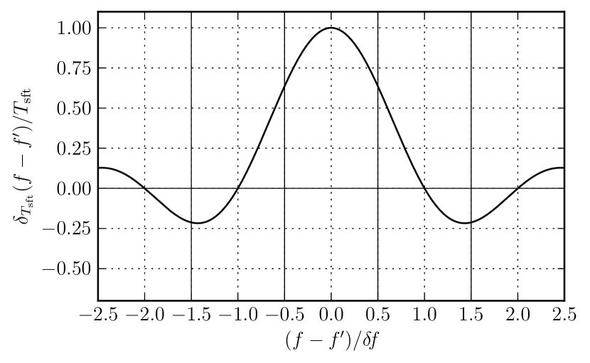
Figure 1: Plot of $\delta_{T_{\text{sft}}}(f-f^{\prime})$ defined in (17) which determines the signal contribution to a given frequency bin of a short Fourier transform (SFT) of duration $T_{\text{sft}}$ according to (16). Since the spacing between frequency bins is $\delta\!f=1/T_{\text{sft}}$, there will be, for a given signal frequency $f_{K}$, one bin whose value of $\kappa_{Kk}=(f_{k}-f_{K})/\delta\!f$ lies between each pair of vertical solid lines.

The signal contribution will be largest in the $\tilde{k}_{K}$th Fourier bin, defined by

$$\tilde{k}_{K}:=\left\lfloor\frac{f_{K}}{\delta\!f}\right\rceil=\left\lfloor f_{K}T_{\text{sft}}\right\rceil$$ (18)

whose frequency $f_{\tilde{k}_{K}}$ is closest to $f_{K}$. (We have introduced the notation that $\left\lfloor\alpha\right\rceil$ is the closest integer to $\alpha$.) It will prove useful to define, similarly to Prix (2011),

$$\kappa_{Kk}=k-f_{K}T_{\text{sft}}=\frac{f_{k}-f_{K}}{\delta\!f}\equiv\tilde{\kappa}_{K}+(k-\tilde{k}_{K})$$ (19)

where

$$\tilde{\kappa}_{K}=\frac{f_{\tilde{k}_{K}}-f_{K}}{\delta\!f}=\tilde{k}_{K}-f_{K}T_{\text{sft}}\ ,$$ (20)

so that $-\frac{1}{2}\leq\tilde{\kappa}_{K}\leq\frac{1}{2}$. A simple search would consider, from each SFT $K$, only the Fourier component $\widetilde{x}_{K\tilde{k}_{K}}$ closest in frequency to the signal frequency $f_{K}$ at the search parameters. However, as we will see, the sensitivity of the search can be improved by including contributions from additional adjacent bins, so we indicate by $\mathcal{K}_{K}$ the set of bins to be considered from SFT $K$, and we will construct a detection statistic using $\widetilde{x}_{Kk}$ for all $k\in\mathcal{K}_{K}$.

We can then write

$$\widetilde{h}_{Kk}\approx h_{0}(-1)^{k}\operatorname{sinc}(\kappa_{Kk})e^{\mathrm{i}\Phi_{K}}\frac{F^{K}_{+}\mathcal{A}_{+}-\mathrm{i}F^{K}_{\times}\mathcal{A}_{\times}}{2}T_{\text{sft}}$$ (21)

which means that, from (10)

$$E\left[z_{K{k}}\right]=\mu_{K{k}}\\ \approx h_{0}(-1)^{k}\operatorname{sinc}(\kappa_{Kk})e^{\mathrm{i}\Phi_{K}}\frac{F^{K}_{+}\mathcal{A}_{+}-\mathrm{i}F^{K}_{\times}\mathcal{A}_{\times}}{2}\sqrt{\frac{2T_{\text{sft}}}{S_{K}}}$$ (22)

II.4 Construction of the cross-correlation statistic

For a given choice of signal parameters, which determine $\tilde{\kappa}_{K}$ for each SFT, and therefore $\kappa_{Kk}$ for each Fourier component, it is useful to define

$$\begin{split}z_{K}&=\frac{\sum_{k\in\mathcal{K}_{K}}(-1)^{k}\operatorname{sinc}(\kappa_{Kk})z_{Kk}}{\sqrt{\sum_{k^{\prime}\in\mathcal{K}_{K}}\operatorname{sinc}^{2}(\kappa_{Kk^{\prime}})}}\\ &\equiv\frac{1}{\Xi_{K}}\sum_{k\in\mathcal{K}_{K}}(-1)^{k}\operatorname{sinc}(\kappa_{Kk})z_{Kk}\end{split}$$ (23)

This is still normalized so that

$$E\left[(z_{K}-\mu_{K})(z_{L}-\mu_{L})^{*}\right]=\delta_{KL}$$ (24a)

$$E\left[(z_{K}-\mu_{K})(z_{L}-\mu_{L})\right]=0$$ (24b)

where now

$$\mu_{K}\approx h_{0}e^{\mathrm{i}\Phi_{K}}\frac{F^{K}_{+}\mathcal{A}_{+}-\mathrm{i}F^{K}_{\times}\mathcal{A}_{\times}}{2}\Xi_{K}\sqrt{\frac{2T_{\text{sft}}}{S_{K}}}$$ (25)

If we define vectors indexed by SFT number, we can write (24) and (25) in matrix form as

$$E\left[\mathbf{z}\right]=\boldsymbol{\mu}$$ (26a)

$$E\left[(\mathbf{z}-\boldsymbol{\mu}){(\mathbf{z}-\boldsymbol{\mu})}^{{\dagger}}\right]=\boldsymbol{1}$$ (26b)

$$E\left[(\mathbf{z}-\boldsymbol{\mu}){(\mathbf{z}-\boldsymbol{\mu})}^{\text{tr}}\right]=\boldsymbol{0}$$ (26c)

where $\boldsymbol{1}$ is the identity matrix, $\boldsymbol{0}$ is a matrix of zeros, ${(\cdot)}^{\text{tr}}$ indicates the matrix transpose and ${(\cdot)}^{{\dagger}}$ the matrix adjoint (complex conjugate of the transpose).

A real cross-correlation statistic $\rho$ can be constructed by defining a Hermitian matrix $\mathbf{W}$ and constructing $\rho={\mathbf{z}}^{{\dagger}}\mathbf{W}\mathbf{z}=\operatorname{Tr}(\mathbf{W}\mathbf{z}{\mathbf{z}}^{{\dagger}})$. [Our chosen form of $\mathbf{W}$ will be defined in (35).] Equation (26) tells us that

$$E\left[\mathbf{z}{\mathbf{z}}^{{\dagger}}\right]=\boldsymbol{1}+\boldsymbol{\mu}{\boldsymbol{\mu}}^{{\dagger}}$$ (27)

where the second term is a matrix with elements

$$\mu_{K}\mu_{L}^{*}=h_{0}^{2}\Xi_{K}\Xi_{L}e^{{\mathrm{i}}\Delta\Phi_{KL}}\Gamma_{KL}\frac{2T_{\text{sft}}}{\sqrt{S_{K}S_{L}}}$$ (28)

where $\Delta\Phi_{KL}=\Phi_{K}-\Phi_{L}$ is the difference between the modeled signal phases in the two SFTs and $\Gamma_{KL}$ is a geometrical factor which depends on $\iota$ and $\psi$ as follows [compare Eq. (3.10) of Dhurandhar et al. (2008)]:

$$\begin{split}\Gamma_{KL}=&\,\frac{1}{4}\bigl{(}F^{K}_{+}F^{L}_{+}\mathcal{A}_{+}^{2}+F^{K}_{\times}F^{L}_{\times}\mathcal{A}_{\times}^{2}\\ &\,\phantom{\frac{1}{4}\bigl{(}}+{\mathrm{i}}[F^{K}_{+}F^{L}_{\times}-F^{K}_{\times}F^{L}_{+}]\mathcal{A}_{+}\mathcal{A}_{\times}\bigr{)}\\ =&\,\frac{1}{4}\biggl{(}\frac{\mathcal{A}_{+}^{2}+\mathcal{A}_{\times}^{2}}{2}\,(a^{K}a^{L}+b^{K}b^{L})\\ &\,+{\mathrm{i}}\,\mathcal{A}_{+}\mathcal{A}_{\times}\,(a^{K}b^{L}-b^{K}a^{L})\\ &\,\phantom{\frac{1}{4}\biggl{(}}+\,\frac{\mathcal{A}_{+}^{2}-\mathcal{A}_{\times}^{2}}{2}\,\bigl{[}(a^{K}a^{L}-b^{K}b^{L})\,\cos 4\psi\\ &\,\phantom{\frac{1}{4}\biggl{(}+\,\frac{\mathcal{A}_{+}^{2}-\mathcal{A}_{\times}^{2}}{2}\,\bigl{[}}+(a^{K}b^{L}+b^{K}a^{L})\,\sin 4\psi\bigr{]}\biggr{)}\end{split}$$ (29)

where we have used the fact that the $\psi$ dependence of the antenna patterns $F^{K}_{+,\times}$ can be written in terms of the amplitude modulation (AM) coefficients $a^{K}$ and $b^{K}$ as

$$F^{K}_{+}\, = a^{K} \,\cos 2\psi\, + \,b^{K}\,\sin 2\psi$$ (30)

$$F^{K}_{\times}\, =-\, a^{K} \,\sin 2\psi\, + \,b^{K}\,\cos 2\psi\ .$$ (31)

The AM coefficientsJaranowski et al. (1998) are determined by the relevant sky position, detector and sidereal time. They can be definedPrix and Whelan (2007) as $a^{K}={\varepsilon}_{+}^{ab}{d}^{K}_{ab}$ and $b^{K}={\varepsilon}_{\times}^{ab}{d}^{K}_{ab}$ where ${\varepsilon}_{+}^{ab}$ and ${\varepsilon}^{ab}_{\times}$ are a polarization basis defined using one basis vector pointing west along a line of constant declination and one pointing north along a line of constant right ascension. Note that $\iota$ and $\psi$ are properties of the source which do not change for different SFT pairs, while $a^{K}$ and $b^{K}$ depend only on the SFT (detector and sidereal time) and sky position. It is also useful to note that the combinations

$$F^{K}_{+}F^{L}_{+}+F^{K}_{\times}F^{L}_{\times} =a^{K}a^{L}+b^{K}b^{L}\equiv 10\Gamma^{\text{ave}}_{KL}$$ (32a)

$$F^{K}_{+}F^{L}_{\times}-F^{K}_{\times}F^{L}_{+} =a^{K}b^{L}-b^{K}a^{L}\equiv 10\Gamma^{\text{circ}}_{KL}$$ (32b)

are independent of $\psi$.

Since terms in $\Gamma_{KL}$ change signs if we vary $\cos\iota$ and $\psi$, which are unknown, it is convenient, as proposed in Dhurandhar et al. (2008), to work with the average over those quantities, which picks out the “robust” part:

$$\Gamma^{\text{ave}}_{KL}=\left\langle\Gamma_{KL}\right\rangle_{\cos\iota,\psi}=\frac{1}{10}(a^{K}a^{L}+b^{K}b^{L})$$ (33)

Note that $\Gamma^{\text{ave}}_{KL}$ is real and non-negative, while $\Gamma_{KL}$ is complex. On the other hand, $\Gamma_{KL}$ can be factored into $\gamma_{K}\gamma_{L}^{*}$, while $\Gamma^{\text{ave}}_{KL}$ cannot. If we define (again as in Prix (2011), but with a different overall normalization) “noise-weighted AM coefficients” $\widehat{a}^{K}$ and $\widehat{b}^{K}$ by dividing by $\sqrt{\frac{S_{K}}{2T_{\text{sft}}}}$ and construct $\widehat{\Gamma}_{KL}$ from those, we can write

$$\mu_{K}\mu_{L}^{*}=h_{0}^{2}\Xi_{K}\Xi_{L}e^{{\mathrm{i}}\Delta\Phi_{KL}}\widehat{\Gamma}_{KL}=h_{0}^{2}\widehat{G}_{KL}$$ (34)

or, as a matrix equation, $\boldsymbol{\mu}{\boldsymbol{\mu}}^{{\dagger}}=h_{0}^{2}\widehat{\mathbf{G}}$. Note that Dhurandhar et al. (2008) did not consider issues of spectral leakage responsible for $\Xi_{K}$, and used a different convention for the placement of complex conjugates in atomic cross-correlation term, so their $\tilde{\mathcal{G}}_{KL}$ would be equal to $\frac{G_{KL}^{*}}{\Xi_{K}\Xi_{L}}$ in the present notation. Similarly, our $\frac{\widehat{G}_{KL}^{*}}{\Xi_{K}\Xi_{L}}$ corresponds to the combination $\frac{\tilde{\mathcal{G}}_{KL}}{\sqrt{\sigma^{2}_{KL}}}$ from Dhurandhar et al. (2008).

As noted in Dhurandhar et al. (2008), an “optimal” combination of cross-correlation terms would use a weight $\mathbf{W}$ proportional to $\widehat{\mathbf{G}}$. However, as described above, we work with $\widehat{G}^{\text{ave}}_{KL}=\Xi_{K}\Xi_{L}e^{{\mathrm{i}}\Delta\Phi_{KL}}\widehat{\Gamma}^{\text{ave}}_{KL}$ in order to avoid specifying the parameters $\cos\iota$ and $\psi$. For reasons of computational cost to be detailed later, we limit the possible set of SFT pairs $KL$ included in the cross-correlation to some set $\mathcal{P}$, in particular by requiring that $K<L$ and $\left\lvert t_{K}-t_{L}\right\rvert<T_{\text{max}}$. Then we define the Hermitian weighting matrix $\mathbf{W}$ by

$$W_{KL}=\begin{cases}N\widehat{G}^{\text{ave}}_{KL}&KL\in\mathcal{P}\\ N(\widehat{G}^{\text{ave}}_{KL})^{*}&LK\in\mathcal{P}\\ 0&\text{otherwise}\end{cases}$$ (35)

so that the cross-correlation statistic is

$$\begin{split}\rho&={\mathbf{z}}^{{\dagger}}\mathbf{W}\mathbf{z}=\operatorname{Tr}(\mathbf{W}\mathbf{z}{\mathbf{z}}^{{\dagger}})\\ &=N\sum_{KL\in\mathcal{P}}\left(\widehat{G}^{\text{ave}}_{KL}z_{K}^{*}z_{L}+\widehat{G}^{\text{ave}\,*}_{KL}z_{K}z_{L}^{*}\right)\\ &=N\sum_{KL\in\mathcal{P}}\widehat{\Gamma}^{\text{ave}}_{KL}\sum_{k\in\mathcal{K}_{K}}\sum_{\ell\in\mathcal{K}_{L}}(-1)^{k-\ell}\operatorname{sinc}(\kappa_{Kk})\operatorname{sinc}(\kappa_{L\ell})\\ &\phantom{N\sum_{KL\in\mathcal{P}}\widehat{\Gamma}^{\text{ave}}_{KL}\sum_{k\in\mathcal{K}_{K}}}\times\left(e^{{\mathrm{i}}\Delta\Phi_{KL}}z_{Kk}^{*}z_{L\ell}+e^{-{\mathrm{i}}\Delta\Phi_{KL}}z_{Kk}z_{L\ell}^{*}\right)\end{split}$$ (36)

Since we assume that the list of pairs $\mathcal{P}$ includes no autocorrelations, the matrix $\mathbf{W}$ contains no diagonal elements, which implies $\operatorname{Tr}(\mathbf{W})=0$. We will later introduce, and use when convenient, the notation that $\alpha$ labels a (nonordered) pair of SFTs $KL\in\mathcal{P}$.

III Statistics and Sensitivity

In this section we consider in detail the statistical properties of the cross-correlation statistic $\rho$ which were sketched in a basic form in Dhurandhar et al. (2008). In particular, we consider the impact on the expected sensitivity of spectral leakage and unknown amplitude parameters, and compare the sensitivity of a cross-correlation search to the directed stochastic search by analogy to which it was defined.

III.1 Mean and variance of cross-correlation statistic

The expectation value of the cross-correlation statistic is

$$\begin{split}E\left[\rho\right]&=E\left[\operatorname{Tr}(\mathbf{W}\mathbf{z}{\mathbf{z}}^{{\dagger}})\right]=\operatorname{Tr}(\mathbf{W})+h_{0}^{2}\operatorname{Tr}(\mathbf{W}\widehat{\mathbf{G}})\\ &=h_{0}^{2}\operatorname{Tr}(\mathbf{W}\widehat{\mathbf{G}})={\boldsymbol{\mu}}^{{\dagger}}\mathbf{W}\boldsymbol{\mu}\end{split}$$ (37)

where we have used the fact that $\mathbf{W}$ is traceless. The variance is

$$\operatorname{Var}(\rho)=E\left[\rho^{2}\right]-E\left[\rho\right]^{2}=E\left[{\mathbf{z}}^{{\dagger}}\mathbf{W}\mathbf{z}{\mathbf{z}}^{{\dagger}}\mathbf{W}\mathbf{z}\right]-({\boldsymbol{\mu}}^{{\dagger}}\mathbf{W}\boldsymbol{\mu})^{2}$$ (38)

The first term can be evaluated by writing $\mathbf{z}=(\mathbf{z}-\boldsymbol{\mu})+\boldsymbol{\mu}$; after some simplification we have

$$\begin{split}\operatorname{Var}(\rho)=&\,E\left[{(\mathbf{z}-\boldsymbol{\mu})}^{{\dagger}}\mathbf{W}(\mathbf{z}-\boldsymbol{\mu}){(\mathbf{z}-\boldsymbol{\mu})}^{{\dagger}}\mathbf{W}(\mathbf{z}-\boldsymbol{\mu})\right]\\ &+2{\boldsymbol{\mu}}^{{\dagger}}\mathbf{W}^{2}\boldsymbol{\mu}\end{split}$$ (39)

Ordinarily we would need to know something about the fourth moment of the noise distribution to evaluate the expectation value, but since $\mathbf{W}$ contains no diagonal elements, and the different elements of $\mathbf{z}-\boldsymbol{\mu}$ are independent of each other, the expectation value can be evaluated using only the variance-covariance matrix of $\mathbf{z}$ to give

$$\operatorname{Var}(\rho)=\operatorname{Tr}{\mathbf{W}^{2}}+2{\boldsymbol{\mu}}^{{\dagger}}\mathbf{W}^{2}\boldsymbol{\mu}=\operatorname{Tr}{\mathbf{W}^{2}}+2h_{0}^{2}\operatorname{Tr}{\mathbf{W}^{2}\widehat{\mathbf{G}}}$$ (40)

We choose the normalization constant $N$ so that $\rho$ has unit variance in the limit $h_{0}^{2}\rightarrow 0$, i.e.,

$$1=\operatorname{Tr}(\mathbf{W}^{2})=\sum_{K}\sum_{L}W_{KL}W_{LK}=2N^{2}\sum_{KL\in\mathcal{P}}\left\lvert\widehat{G}^{\text{ave}}_{KL}\right\rvert^{2}$$ (41)

i.e.,

$$N^{-2}=2\sum_{KL\in\mathcal{P}}\left\lvert\widehat{G}^{\text{ave}}_{KL}\right\rvert^{2}=2\sum_{KL\in\mathcal{P}}\Xi_{K}^{2}\Xi_{L}^{2}\left(\widehat{\Gamma}^{\text{ave}}_{KL}\right)^{2}$$ (42)

Written in terms of SFT pairs, the expectation value of the statistic is

$$\begin{split}E\left[\rho\right]&=h_{0}^{2}\operatorname{Tr}(\mathbf{W}\widehat{\mathbf{G}})\\ &=Nh_{0}^{2}\sum_{KL\in\mathcal{P}}\left(\widehat{G}^{\text{ave}}_{KL}\widehat{G}_{KL}^{*}+\widehat{G}^{\text{ave}\,*}_{KL}\widehat{G}_{KL}\right)\\ &=Nh_{0}^{2}\,2\sum_{KL\in\mathcal{P}}\Xi_{K}^{2}\Xi_{L}^{2}\widehat{\Gamma}^{\text{ave}}_{KL}\operatorname{Re}\widehat{\Gamma}_{KL}\end{split}$$ (43)

Looking at (29) we see that the real part of $\Gamma_{KL}$ has a piece proportional to $\Gamma^{\text{ave}}_{KL}$ and a piece that depends on $\psi$:

$$\operatorname{Re}\Gamma_{KL}=\frac{5}{2}\frac{\mathcal{A}_{+}^{2}+\mathcal{A}_{\times}^{2}}{2}\Gamma^{\text{ave}}_{KL}+\frac{\mathcal{A}_{+}^{2}-\mathcal{A}_{\times}^{2}}{2}(F^{K}_{+}F^{L}_{+}-F^{K}_{\times}F^{L}_{\times})$$ (44)

The sum over SFT pairs $KL$ can be broken down as a sum over detector pairs, over time offsets $t_{K}-t_{L}$, and over the time stamp $\frac{1}{2}(t_{K}+t_{L})$ halfway between the time stamps of the SFTs in the pair. In an idealized long observing run, if the detector noise is uncorrelated with sidereal time, the sum over $\frac{1}{2}(t_{K}+t_{L})$ means we are averaging the two expressions $(a^{K}a^{L}+b^{K}b^{L})^{2}$ and $(a^{K}a^{L}+b^{K}b^{L})(F^{K}_{+}F^{L}_{+}-F^{K}_{\times}F^{L}_{\times})$ (the latter of which depends on the polarization angle $\psi$) over sidereal time. Because the former is positive definite and the latter is not, this average tends to suppress the $\psi$-dependent term. This is in addition to the fact that $\frac{\mathcal{A}_{+}^{2}+\mathcal{A}_{\times}^{2}}{2}\geq\frac{\mathcal{A}_{+}^{2}-\mathcal{A}_{\times}^{2}}{2}$, possibly substantially, depending on the value of $\iota$, as illustrated in Fig. 2.

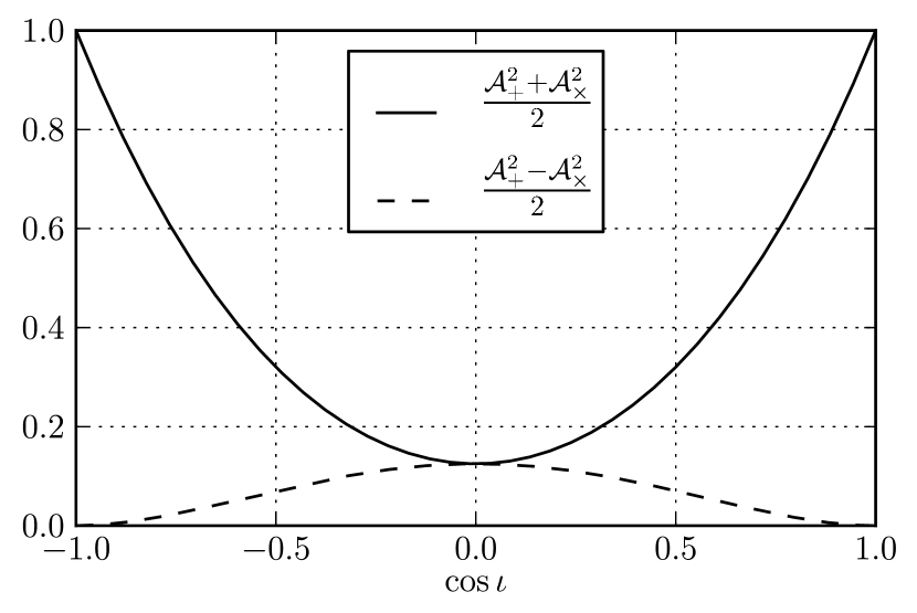
Figure 2: Plot of $\frac{\mathcal{A}_{+}^{2}+\mathcal{A}_{\times}^{2}}{2}$ and $\frac{\mathcal{A}_{+}^{2}-\mathcal{A}_{\times}^{2}}{2}$, the coefficients of the two contributions to $\operatorname{Re}\Gamma_{KL}$ in (44). The factor $\frac{\mathcal{A}_{+}^{2}+\mathcal{A}_{\times}^{2}}{2}$ is also equal to $\frac{2}{5}\frac{(h^{\text{eff}}_{0})^{2}}{h_{0}^{2}}$ where $(h^{\text{eff}}_{0})^{2}$ is the combination of $h_{0}$ and $\cos\iota$ approximately measured by the cross-correlation statistic, as shown in, e.g., Eq. (45)

If we neglect the second term in (44), (43) becomes

$$\begin{split}E\left[\rho\right]&\approx Nh_{0}^{2}\frac{5}{2}\frac{\mathcal{A}_{+}^{2}+\mathcal{A}_{\times}^{2}}{2}2\sum_{KL\in\mathcal{P}}\Xi_{K}^{2}\Xi_{L}^{2}\left(\widehat{\Gamma}^{\text{ave}}_{KL}\right)^{2}\\ &=(h^{\text{eff}}_{0})^{2}\sqrt{2\sum_{KL\in\mathcal{P}}\Xi_{K}^{2}\Xi_{L}^{2}\left(\widehat{\Gamma}^{\text{ave}}_{KL}\right)^{2}}\end{split}$$ (45)

where

$$h_{0}^{\text{eff}}=h_{0}\sqrt{\frac{5}{2}\frac{\mathcal{A}_{+}^{2}+\mathcal{A}_{\times}^{2}}{2}}$$ (46)

is the combination of $h_{0}$ and $\cos\iota$ that we can estimate by filtering with the averaged template.

Since we have normalized the statistic so that $\operatorname{Var}(\rho)=1$ for weak signals, the expectation value (45) is an expected signal-to-noise ratio for a signal with a given $h_{0}^{\text{eff}}$. This means that if we define a SNR threshold $\rho^{\text{th}}$ such that $\rho>\rho^{\text{th}}$ corresponds to a detection, the signal will be detectable if

$$h_{0}^{\text{eff}}\gtrsim\sqrt{\rho^{\text{th}}}\left(2\sum_{KL\in\mathcal{P}}\Xi_{K}^{2}\Xi_{L}^{2}\left(\widehat{\Gamma}^{\text{ave}}_{KL}\right)^{2}\right)^{-1/4}$$ (47)

III.2 Impact of spectral leakage on estimated sensitivity

Finally, we consider the impact of the leakage factors of the form $\Xi_{K}^{2}=\sum_{k\in\mathcal{K}_{K}}\operatorname{sinc}^{2}(\kappa_{Kk})$ on the expectation value. Expanding these expressions, we have

$$E\left[\rho\right]\approx(h^{\text{eff}}_{0})^{2}\biggl{(}2\sum_{KL\in\mathcal{P}}\left(\widehat{\Gamma}^{\text{ave}}_{KL}\right)^{2}\\ \times\sum_{k\in\mathcal{K}_{K}}\operatorname{sinc}^{2}(\kappa_{Kk})\sum_{\ell\in\mathcal{K}_{L}}\operatorname{sinc}^{2}(\kappa_{L\ell})\biggr{)}^{1/2}$$ (48)

If we choose only the “best bin” $k_{K}=\tilde{k}_{K}$ from each SFT, defined by (18), we have

$$\Xi_{K}^{2}=\operatorname{sinc}^{2}(\tilde{\kappa}_{K})$$ (49)

If, instead of the best bin whose frequency $f_{\tilde{k}_{K}}$ is closest to $f_{K}$, we take the $m$ closest bins to define $\mathcal{K}_{K}$, the sum becomes

$$\begin{split}\Xi_{K}^{2}&=\sum_{k\in\mathcal{K}_{K}}\operatorname{sinc}^{2}(\kappa_{Kk})=\sum_{k=\tilde{k}_{K}-\left\lceil(m-1)/2\right\rceil}^{\tilde{k}_{K}+\left\lfloor(m-1)/2\right\rfloor}\operatorname{sinc}^{2}(\kappa_{Kk})\\ &=\sum_{s=-\left\lceil(m-1)/2\right\rceil}^{\left\lfloor(m-1)/2\right\rfloor}\operatorname{sinc}^{2}(\tilde{\kappa}_{K}+s)\end{split}$$ (50)

where $\left\lfloor\alpha\right\rfloor\leq\alpha$ and $\left\lceil\alpha\right\rceil\geq\alpha$ are the integers below and above $\alpha$, respectively. Note that, because of the identity $\sum_{s=-\infty}^{\infty}\operatorname{sinc}^{2}(\kappa+s)=1$, valid for any $\kappa$, the best we can do by including more bins is $\Xi_{K}^{2}\leq 1$ and therefore

$$E\left[\rho\right]\leq(h^{\text{eff}}_{0})^{2}\sqrt{2\sum_{KL\in\mathcal{P}}\left(\widehat{\Gamma}^{\text{ave}}_{KL}\right)^{2}}$$ (51)

The sensitivity associated with the inclusion of a finite number of bins from each SFT will depend on the value of $-\frac{1}{2}\leq\tilde{\kappa}_{K}\leq\frac{1}{2}$ corresponding to the signal frequency $f_{K}$ in each SFT. We can get an estimate of this by assuming that, over the course of the analysis, the Doppler shift evenly samples the range of $\tilde{\kappa}$ values, and writing

$$\begin{split}E\left[\rho\right]&\approx(h^{\text{eff}}_{0})^{2}\sqrt{2\langle\Xi^{2}\rangle^{2}\sum_{KL\in\mathcal{P}}\left(\widehat{\Gamma}^{\text{ave}}_{KL}\right)^{2}}\\ &=(h^{\text{eff}}_{0})^{2}\langle\Xi^{2}\rangle\sqrt{2\sum_{KL\in\mathcal{P}}\left(\widehat{\Gamma}^{\text{ave}}_{KL}\right)^{2}}\end{split}$$ (52)

with

$$\langle\Xi^{2}\rangle=\left\langle\sum_{s}\operatorname{sinc}^{2}(\kappa+s)\right\rangle_{\kappa}$$ (53)

where $\langle\cdot\rangle_{\kappa}$ indicates an average over the possible offsets within the bin. We can numerically evaluate

$$\begin{split}\langle\Xi^{2}\rangle&=\sum_{s}\left\langle\operatorname{sinc}^{2}(\kappa+s)\right\rangle_{\kappa}\\ &=\sum_{s=-\left\lceil(m-1)/2\right\rceil}^{\left\lfloor(m-1)/2\right\rfloor}2\int_{0}^{1/2}\operatorname{sinc}^{2}(\kappa+s)\,d\kappa\\ &=2\int_{0}^{m/2}\operatorname{sinc}^{2}\!\kappa\,d\kappa\end{split}$$ (54)

as shown in Table 2.

Table 2: Contributions to $\langle\Xi^{2}\rangle$, defined in (54), from inclusion of multiple SFT bins. We see that using a single bin from each SFT leads to only around 77.4% of the maximum sensitivity given by (51), but that we can recover over 90% of this sensitivity by using two bins and over 95% by using four bins from each SFT. This table applies for rectangularly windowed data; using other window options further reduces the expected SNR, as described in Appendix A. The table also assumes that the various Doppler modulations move the signal frequency around to accomplish an average over the fractional offset of the signal frequency from the center of the bin. The validity of this approximation is explored in Sundaresan and Whelan (2012).

$m$	1	2	3	4	5	6
Contribution	0.774	0.129	0.028	0.019	0.009	0.007
Cumulative	0.774	0.903	0.931	0.950	0.959	0.966

Since most cross-correlation searches will be computationally limited, the question of how many bins to include from each SFT is one of optimization of resources. The value of $E\left[\rho\right]$ for a given $h^{\text{eff}}_{0}$, and therefore the sensitivity of the search, can be increased by including more frequency bins from each SFT, but this will involve more computations and therefore more computational resources. If instead those resources were put into a search with a larger $T_{\text{max}}$, the value of $\sum_{KL\in\mathcal{P}}\left(\widehat{\Gamma}^{\text{ave}}_{KL}\right)^{2}$ would be higher. Naively, one might expect the computing cost to scale with the number of terms to be combined, and therefore with the square of the number of bins taken from each SFT. So increasing from $m=1$ to $m=2$ could take up to $4$ times the computing cost. On the other hand, for a fixed number of bins, we suppose that the cost will scale with the number of SFT pairs to be included times the number of parameter space points to be searched. Typical behavior will be for the density of points in parameter space to scale with $T_{\text{max}}^{d}$ for some integer value of $d$; as described in Sec. IV.2, for a search over frequency and two orbital parameters of an LMXB, as long as $T_{\text{max}}$ is small compared to the binary orbital period, $d=3$. Since the number of SFT pairs at fixed observation time will also scale like $T_{\text{max}}$, the overall computing cost will scale like $T_{\text{max}}^{d+1}$, and quadrupling the computing time would mean multiplying the possible $T_{\text{max}}$, and thus the number of terms in the sum (52) by $4^{\frac{1}{d+1}}$. This would increase $E\left[\rho\right]$ for a given $h^{\text{eff}}_{0}$ by a factor of $4^{\frac{1}{2(d+1)}}=2^{\frac{1}{d+1}}$. For $d=3$, this is $2^{1/4}\approx 1.19$, which is very slightly more than the benefit $\frac{0.903}{0.774}\approx 1.17$ from including a second bin from each SFT. However, the assumption that computing cost scales like $m^{2}$ is likely an overestimate (since most of the operations can be done once per SFT rather than once per pair), so it is generally advisable to use at least two bins from each SFT.

III.3 Sensitivity estimate for unknown amplitude parameters

The cross-correlation statistic is normalized so that $\operatorname{Var}(\rho)\approx 1$ and, according to (52), and now adopting the notation that $\alpha$ refers to an unordered allowed pair of SFTs,

$$E\left[\rho\right]=(h^{\text{eff}}_{0})^{2}\langle\Xi^{2}\rangle\sqrt{2\sum_{\alpha}\left(\widehat{\Gamma}^{\text{ave}}_{\alpha}\right)^{2}}=(h^{\text{eff}}_{0})^{2}\varrho^{\text{ave}}$$ (55)

where $h^{\text{eff}}_{0}$ is the combination of $h_{0}$ and $\cos\iota$ given in (46), and $\varrho^{\text{ave}}$ is a property of the search which can be determined from noise spectra, AM coefficients, and choices of SFT pairs, without knowledge of signal parameters other than the approximate frequency and orbital parameters. Even if the noise in each data stream is Gaussian distributed, the statistic, which combines the data quadratically, will not be. It was observed in Dhurandhar et al. (2008) that each individual cross correlation between SFTs is Bessel distributed; the of the optimal sum is considered in Appendix B both in its exact form and a numerical approximation. For simplicity, in what follows we assume that the central limit theorem allows us to treat the statistic as approximately Gaussian, with mean $(h^{\text{eff}}_{0})^{2}\varrho^{\text{ave}}$ and unit variance.

We consider the sensitivity estimates in Dhurandhar et al. (2008), which implicitly assume the values of $\iota$ and $\psi$ are known and used to construct the expected cross correlation used in weighting the terms in the statistic. [In our notation this would mean using $\widehat{G}_{KL}$ rather than $\widehat{G}^{\text{ave}}_{KL}$ in the definition (35) of $\mathbf{W}$.] Here we perform the analogous calculation, assuming we’re using $\widehat{G}^{\text{ave}}_{\alpha}$ in the construction of the statistic. Thus the probability of exceeding a threshold $\rho^{\text{th}}$ will be

$$P(\rho>\rho^{\text{th}}|h_{0},\iota,\psi)=\int_{\rho^{\text{th}}}^{\infty}f(\rho|h_{0},\iota,\psi)\,d\rho\\ \approx\frac{1}{\sqrt{2\pi}}\int_{\rho^{\text{th}}}^{\infty}\exp\left(-\frac{1}{2}\left[\rho-(h^{\text{eff}}_{0})^{2}\varrho^{\text{ave}}\right]^{2}\right)\,d\rho\\ =\frac{1}{2}\operatorname{erfc}\left(\frac{\rho^{\text{th}}-(h^{\text{eff}}_{0})^{2}\varrho^{\text{ave}}}{\sqrt{2}}\right)=\frac{1}{2}\operatorname{erfc}\left(\frac{\rho^{\text{th}}-h_{0}^{2}\varrho(\iota)}{\sqrt{2}}\right)$$ (56)

where

$$\varrho(\iota)\approx\frac{5}{2}\frac{\mathcal{A}_{+}^{2}+\mathcal{A}_{\times}^{2}}{2}\varrho^{\text{ave}}=\frac{5}{16}(1+6\cos^{2}\iota+\cos^{4}\iota)\varrho^{\text{ave}}$$ (57)

The threshold associated with a false alarm probability $\alpha$ is

$$\rho^{\text{th}}=\sqrt{2}\operatorname{erfc}^{-1}(2\alpha)$$ (58)

but the sensitivity $h_{0}^{\text{sens}}$ associated with a false dismissal probability $\beta$ will now be defined, following a procedure analogous to the one in Wette (2012), by marginalizing over the unknown inclination $\iota$ (since we have neglected the $\psi$ dependence in $E\left[\rho\right]$)

$$\begin{split}1-\beta&=P(\rho>\rho^{\text{th}}|h_{0}=h_{0}^{\text{sens}})\\ &=\left\langle P(\rho>\rho^{\text{th}}|h_{0}=h_{0}^{\text{sens}},\iota,\psi)\right\rangle_{\cos\iota,\psi}\\ &=\frac{1}{2}\left\langle\operatorname{erfc}\left(\frac{\rho^{\text{th}}-(h_{0}^{\text{sens}})^{2}\,\varrho(\iota)}{\sqrt{2}}\right)\right\rangle_{\cos\iota}\end{split}$$ (59)

So to get a sensitivity estimate, we need to find the $h_{0}^{\text{sens}}$ which solves (59), i.e.,

$$2(1-\beta)\\ \approx\left\langle\operatorname{erfc}\left(\frac{\rho^{\text{th}}}{\sqrt{2}}-\frac{(h_{0}^{\text{sens}})^{2}\,\varrho^{\text{ave}}}{\sqrt{2}}\frac{5}{16}(1+6\cos^{2}\iota+\cos^{4}\iota)\right)\right\rangle_{\cos\iota}\\ =\int_{0}^{1}\operatorname{erfc}\left(\operatorname{erfc}^{-1}(2\alpha)-\mathcal{S}^{\text{eff}}\frac{5}{16}\left[1+6\chi^{2}+\chi^{4}\right]\right)\,d\chi$$ (60)

so that the approximate sensitivity is

$$h_{0}^{\text{sens}}=\sqrt{\frac{\mathcal{S}^{\text{eff}}\sqrt{2}}{\varrho^{\text{ave}}}}=\left((\mathcal{S}^{\text{eff}})^{-2}\langle\Xi^{2}\rangle^{2}\sum_{\alpha}\left(\widehat{\Gamma}^{\text{ave}}_{\alpha}\right)^{2}\right)^{-1/4}$$ (61)

Equation (60) defines $\mathcal{S}^{\text{eff}}$ as a specific function of $\alpha$ and $\beta$, so the approximate sensitivity correction due to marginalizing over $\cos\iota$ can be worked out independently of the details of the search.

Table 3: Approximate modification of search sensitivity, as a function of desired false alarm probability $\alpha$ (corresponding to a statistic threshold of $\rho^{\text{th}}$) and false dismissal probability $\beta$, resulting from filtering with a template averaged over the signal parameters $\cos\iota$ and $\psi$. (The second set of $\alpha$ values is chosen to correspond to interesting single-template false alarm probabilities with a trials factor of $10^{8}$.) The detectable signal amplitude $h_{0}^{\text{sens}}$ (61) is proportional to $\sqrt{\mathcal{S}^{\text{eff}}}$. The table shows, for a variety of choices of $\alpha$ and $\beta$, how the corrected factor $\sqrt{\mathcal{S}^{\text{eff}}}$ calculated according to (60) compares to the standard expression $\mathcal{S}=\operatorname{erfc}^{-1}(2\alpha)+\operatorname{erfc}^{-1}(2\beta)$ which would apply from filtering with known values of the parameters $\cos\iota$ and $\psi$. Note that using the worst-case value $\cos\iota=0$ shows that $1<\mathcal{S}^{\text{eff}}/\mathcal{S}<3.2$.

		$\mathcal{S}$			$\mathcal{S}^{\text{eff}}$			$\sqrt{\mathcal{S}^{\text{eff}}/\mathcal{S}}$
		$\beta$			$\beta$			$\beta$
$\alpha$	$\rho^{\text{th}}$	$0.10$	$0.05$	$0.01$	$0.10$	$0.05$	$0.01$	$0.10$	$0.05$	$0.01$
$0.10$	$1.3$	$1.81$	$2.07$	$2.55$	$3.49$	$4.45$	$6.27$	$1.39$	$1.47$	$1.57$
$0.05$	$1.6$	$2.07$	$2.33$	$2.81$	$4.15$	$5.16$	$7.03$	$1.42$	$1.49$	$1.58$
$0.01$	$2.3$	$2.55$	$2.81$	$3.29$	$5.42$	$6.52$	$8.47$	$1.46$	$1.52$	$1.60$
$10^{-9}$	$6.0$	$5.15$	$5.40$	$5.89$	$12.73$	$14.16$	$16.40$	$1.57$	$1.62$	$1.67$
$5\times 10^{-10}$	$6.1$	$5.23$	$5.48$	$5.96$	$12.96$	$14.40$	$16.64$	$1.57$	$1.62$	$1.67$
$10^{-10}$	$6.4$	$5.40$	$5.66$	$6.14$	$13.48$	$14.93$	$17.20$	$1.58$	$1.62$	$1.67$

We show some sample values Table 3 for $\alpha$ and $\beta$ values between $1\%$ and $10\%$, and also for single-template $\alpha$ values corresponding to overall false alarm probabilities in the same range, assuming a trials factor of $10^{8}$. We see that the $h_{0}$ sensitivity is modified by between $39\%$ and $67\%$ in these cases.

III.4 Scaling and comparison to directed stochastic search

We consider here the behavior of (61) (or equivalently (55)) with parameters such as the observing time $T_{\text{obs}}$ and allowed lag time $T_{\text{max}}$, which is effectively a coherence time. As noted in Dhurandhar et al. (2008), the detectable (61) scales like one over the fourth root of the number of SFT pairs included in the sum $\sum_{\alpha}$:

$$\begin{split}h_{0}^{\text{sens}}&=\left((\mathcal{S}^{\text{eff}})^{-2}\langle\Xi^{2}\rangle^{2}N_{\text{pairs}}\langle(\widehat{\Gamma}^{\text{ave}}_{\alpha})^{2}\rangle\right)^{-1/4}\\ &=\left(N_{\text{pairs}}T_{\text{sft}}^{2}(\mathcal{S}^{\text{eff}})^{-2}\langle\Xi^{2}\rangle^{2}\left\langle\frac{4(\Gamma^{\text{ave}}_{KL})^{2}}{S_{K}S_{L}}\right\rangle\right)^{-1/4}\end{split}$$ (62)

The approximate number of pairs for a search of data from $N_{\text{det}}$ detectors, each with observing time $T_{\text{obs}}$ (so that the total observation time is $N_{\text{det}}T_{\text{obs}}$), with maximum lag time $T_{\text{max}}>T_{\text{sft}}$ is

$$N_{\text{pairs}}\approx N_{\text{det}}^{2}\frac{T_{\text{obs}}}{T_{\text{sft}}}\frac{T_{\text{max}}}{T_{\text{sft}}}$$ (63)

so the sensitivity scaling is

$$h_{0}^{\text{sens}}\sim\left(N_{\text{det}}^{2}T_{\text{obs}}T_{\text{max}}(\mathcal{S}^{\text{eff}})^{-2}\langle\Xi^{2}\rangle^{2}\left\langle\frac{4(\Gamma^{\text{ave}}_{KL})^{2}}{S_{K}S_{L}}\right\rangle\right)^{-1/4}$$ (64)

We wish to compare this sensitivity to that of the directed stochastic search (also known as the “radiometer” method) defined in Ballmer (2006) and used to set limits on gravitational radiation from Sco X-1Abbott et al. (2007b); Abadie et al. (2011). The directed stochastic search is also an optimally weighted cross-correlation search, but only includes contributions from data taken by different detectors at the same time. We first consider the sensitivity of a cross-correlation search using our method with this restriction, and then relate this to the sensitivity of the actual directed stochastic search. If we only allow simultaneous pairs of SFTs, the number of pairs included in the sum (61) becomes

$$N_{\text{pairs}}^{\text{simul}}\approx N_{\text{det}}(N_{\text{det}}-1)\frac{T_{\text{obs}}}{T_{\text{sft}}}$$ (65)

which makes the signal strength to which the search is sensitive

$$(h_{0}^{\text{sens}})^{\text{simul}}\\ \sim\left(N_{\text{det}}(N_{\text{det}}-1)T_{\text{obs}}T_{\text{sft}}(\mathcal{S}^{\text{eff}})^{-2}\langle\Xi^{2}\rangle^{2}\left\langle\frac{4(\Gamma^{\text{ave}}_{KL})^{2}}{S_{K}S_{L}}\right\rangle\right)^{-1/4}\\ \sim h_{0}^{\text{sens}}\left(\left[1-\frac{1}{N_{\text{det}}}\right]\frac{T_{\text{sft}}}{T_{\text{max}}}\right)^{-1/4}$$ (66)

The directed stochastic search is not quite the same as this hypothetical cross-correlation search with simultaneous SFTs, however. Most of these differences are irrelevant or produce effectively identical calculations. For instance, since the $\Delta t_{\alpha}$ appearing in (84) is zero for simultaneous SFTs, the phase difference $\Delta\Phi_{\alpha}=2\pi f_{0}\Delta d_{\alpha}$ just encodes the difference in arrival times at the two detectors. Likewise, while the stochastic search assumes a random unpolarized signal rather than the periodic signal from a neutron star with unknown parameters, this has the same effect as our choice to use $\Gamma^{\text{ave}}_{KL}$ as the geometrical weighting factor. In fact (as noted in Dhurandhar et al. (2008)) $e^{{\mathrm{i}}\Delta\Phi_{KL}}\widehat{\Gamma}^{\text{ave}}_{KL}$ is, up to a normalization, the overlap reduction function for the directed stochastic search. The one significant difference is that, since the stochastic search does not model the orbital Doppler modulation, it does not have access to the signal frequency $f_{K}$ corresponding to SFT $K$, and therefore cannot localize the expected signal frequency to a bin of width $\delta\!f=\frac{1}{T_{\text{sft}}}$. Thus, instead of the optimal combination described by (23) or (36), it must sum with equal weights the contributions $z_{Kk}z^{*}_{Lk}$ across a coarse frequency bin of width $\Delta f\gtrsim\frac{2\pi a_{p}}{P_{\text{orb}}}f_{0}$ (see (IV.2.2) for the definitions of the binary orbital parameters relevant to Doppler modulation). The effect is to increase the variance of the cross correlation due to noise by $\frac{\Delta{f}}{\delta\!f}=\Delta{f}\,T_{\text{sft}}$ (since there are $\Delta{f}\,T_{\text{sft}}$ bins being combined, only one of which contains a significant signal contribution) so that

$$(h_{0}^{\text{sens}})^{\text{stoch}}\\ \sim\left(N_{\text{det}}(N_{\text{det}}-1)\frac{T_{\text{obs}}}{\Delta f}(\mathcal{S}^{\text{eff}})^{-2}\left\langle\frac{4(\Gamma^{\text{ave}}_{KL})^{2}}{S_{K}S_{L}}\right\rangle\right)^{-1/4}\\ \sim h_{0}^{\text{sens}}\left(\langle\Xi^{2}\rangle^{-2}\left[1-\frac{1}{N_{\text{det}}}\right]\frac{1}{\Delta fT_{\text{max}}}\right)^{-1/4}$$ (67)

The appearance of the factor containing $\langle\Xi^{2}\rangle$ in the comparison is because the directed stochastic search, by combining a larger range of frequency bins, as well as techniques such as overlapping windowed segments, avoids some of the usual leakage issues. On the other hand, if $\Delta f$ is chosen to maximize the sensitivity for a given frequency, there will be similar issues with part of the signal falling outside the coarse bin at the extremes of Doppler modulation.

To insert concrete numbers, (67) tells us that for a search with data of equivalent sensitivity from three detectors, a cross-correlation search with $T_{\text{max}}=3600\text{\,s}$ and $\langle\Xi^{2}\rangle=0.9$ would provide an improvement in $h_{0}$ sensitivity over a directed stochastic search with $\Delta f=0.25\text{\,Hz}$ of a factor of about $5.4$. This is consistent with the performance of the two searches in the Sco X-1 Mock Data ChallengeMessenger et al. (2015), in which the cross-correlation method was able to detect signals with $h_{0}$ almost an order of magnitude lower than those detected by the directed stochastic method.

Note that, unlike the model-based cross-correlation search, the stochastic search is not computationally limited, with year-long wide-band analyses being achievable on a single CPUMessenger et al. (2015). Additionally, since it does not assume a signal model (beyond sky localization and approximate monochromaticity), it is robust against unexpected features such as orbital parameters outside the nominally expected range. However, its sensitivity is fundamentally limited by its ignorance of orbital Doppler modulation, with a maximum effective coherence time of $\frac{1}{\Delta f}\lesssim\frac{P_{\text{orb}}}{2\pi{}a_{p}f_{0}}\approx\left(\frac{100\text{\,Hz}}{f_{0}}\right)75\text{\,sec}$.

IV Parameter space behavior

So far we have implicitly assumed the parameters used to construct the signal model (16), other than the amplitude parameters $h_{0}$, $\cos\iota$, and $\psi$, were known when constructing the weighted statistic. In order to determine the phase evolution of the signal, and therefore $\Phi_{K}$ and $f_{K}$, we need various phase-evolution parameters $\{\lambda_{i}\}$. (For example, for a neutron star at a known sky location with a constant intrinsic signal frequency $f_{0}$ in a binary orbit, these are $f_{0}$ and any unknown binary orbital parameters.) A slight error in these would lead to the $\Phi_{K}$ appearing in $\boldsymbol{\mu}$ and that used to construct $\mathbf{W}$ being slightly different. In this case we need to go back to (43) and distinguish between the true $\Delta\Phi_{KL}$ and the one assumed in the construction of the filter. If we write these parameters as $\{\lambda_{i}\}$, let the parameters assumed in constructing $\rho$ be $\lambda_{i}$ and the true parameters of the signal be $\lambda_{i}^{s}$. Let $\Delta\Phi_{KL}^{s}$ and $\Delta\Phi_{KL}$ be the phase difference $\Phi_{K}-\Phi_{L}$ constructed with the true signal parameters and the parameters assumed in $\mathbf{W}$, respectively. The effect will be to reduce the expected SNR $E\left[\rho\right]$ from the value given in (55) which it would attain with $\lambda_{i}=\lambda_{i}^{s}$. The modified value is

$$E[\rho]\approx h_{0}^{2}N\langle\Xi^{2}\rangle\\ \times\sum_{\alpha}\left(\widehat{\Gamma}_{\alpha}e^{\mathrm{i}(\Delta\Phi_{\alpha}^{s}-\Delta\Phi_{\alpha})}+\widehat{\Gamma}_{\alpha}^{*}e^{-\mathrm{i}(\Delta\Phi_{\alpha}^{s}-\Delta\Phi_{\alpha})}\right)\widehat{\Gamma}^{\text{ave}}_{\alpha}$$ (68)

Now, for $\lambda_{i}$ close to $\lambda_{i}^{s}$,

$$\widehat{\Gamma}_{\alpha}e^{\mathrm{i}(\Delta\Phi_{\alpha}^{s}-\Delta\Phi_{\alpha})}+\widehat{\Gamma}_{\alpha}^{*}e^{-\mathrm{i}(\Delta\Phi_{\alpha}^{s}-\Delta\Phi_{\alpha})}\\ =2\operatorname{Re}\widehat{\Gamma}_{\alpha}\cos(\Delta\Phi_{\alpha}^{s}-\Delta\Phi_{\alpha})-2\operatorname{Im}\widehat{\Gamma}_{\alpha}\sin(\Delta\Phi_{\alpha}^{s}-\Delta\Phi_{\alpha})\\ \approx 2\operatorname{Re}\widehat{\Gamma}_{\alpha}\left(1-\frac{1}{2}(\Delta\Phi_{\alpha}-\Delta\Phi_{\alpha}^{s})^{2}\right)+2\operatorname{Im}\widehat{\Gamma}_{\alpha}(\Delta\Phi_{\alpha}-\Delta\Phi_{\alpha}^{s})$$ (69)

if we write the phase difference as

$$\begin{split}\Delta\Phi_{\alpha}-\Delta\Phi_{\alpha}^{s}\approx\ &\sum_{i}\Delta\Phi_{\alpha,i}(\lambda_{i}-\lambda_{i}^{s})\\ &+\frac{1}{2}\sum_{i,j}\Delta\Phi_{\alpha,ij}(\lambda_{i}-\lambda_{i}^{s})(\lambda_{j}-\lambda_{j}^{s})\end{split}$$ (70)

where $\Delta\Phi_{\alpha,i}=\frac{\partial\Phi_{\alpha}}{\partial\lambda_{i}}$, we obtain, to second order in the parameter difference,

$$E\left[\rho\right]\approx(h_{0})^{2}N\langle\Xi^{2}\rangle\left(2\sum_{\alpha}\widehat{\Gamma}^{\text{ave}}_{\alpha}\operatorname{Re}\widehat{\Gamma}_{\alpha}\right)\\ \times\left[1-\sum_{i}\epsilon^{s}_{i}(\lambda_{i}-\lambda_{i}^{s})-\sum_{i,j}g_{ij}(\lambda_{i}-\lambda_{i}^{s})(\lambda_{j}-\lambda_{j}^{s})\right]$$ (71)

where

$$\epsilon^{s}_{i}=-\frac{2\sum_{\alpha}\widehat{\Gamma}^{\text{ave}}_{\alpha}\operatorname{Im}\widehat{\Gamma}_{\alpha}\Delta\Phi_{\alpha,i}}{2\sum_{\alpha}\widehat{\Gamma}^{\text{ave}}_{\alpha}\operatorname{Re}\widehat{\Gamma}_{\alpha}}$$ (72)

and the parameter space metric is

$$g_{ij}=\frac{1}{2}\frac{2\sum_{\alpha}\widehat{\Gamma}^{\text{ave}}_{\alpha}\left(\operatorname{Re}\widehat{\Gamma}_{\alpha}\Delta\Phi_{\alpha,i}\Delta\Phi_{\alpha,j}+\operatorname{Im}\widehat{\Gamma}_{\alpha}\Delta\Phi_{\alpha,ij}\right)}{2\sum_{\alpha}\widehat{\Gamma}^{\text{ave}}_{\alpha}\operatorname{Re}\widehat{\Gamma}_{\alpha}}$$ (73)

If we once again neglect the $\psi$-dependent piece of $\operatorname{Re}\widehat{\Gamma}_{\alpha}$ as well as the second derivative term in the metric, we have

$$\begin{split}g_{ij}&\approx\frac{1}{2}\frac{\sum_{KL\in\mathcal{P}}(\widehat{a}^{K}\widehat{a}^{L}+\widehat{b}^{K}\widehat{b}^{L})^{2}\Delta\Phi_{\alpha,i}\Delta\Phi_{\alpha,j}}{\sum_{KL\in\mathcal{P}}(\widehat{a}^{K}\widehat{a}^{L}+\widehat{b}^{K}\widehat{b}^{L})^{2}}\\ &=\frac{1}{2}\frac{\sum_{\alpha}\widehat{\Gamma}^{\text{ave}}_{\alpha}\Delta\Phi_{\alpha,i}\Delta\Phi_{\alpha,j}}{\sum_{KL\in\mathcal{P}}\widehat{\Gamma}^{\text{ave}}_{\alpha}}=\frac{1}{2}\langle\Delta\Phi_{\alpha,i}\Delta\Phi_{\alpha,j}\rangle_{\alpha}\end{split}$$ (74)

where $\langle\cdot\rangle_{\alpha}$ indicates a weighted average with weighting factor $\left(\widehat{\Gamma}^{\text{ave}}_{\alpha}\right)^{2}$ [recall $\widehat{\Gamma}^{\text{ave}}_{KL}\propto\left(\frac{a_{K}a_{L}+b_{K}b_{L}}{S_{K}S_{L}}\right)^{2}$] and

$$\epsilon^{s}_{i}\approx\frac{2\mathcal{A}_{+}\mathcal{A}_{\times}}{\mathcal{A}_{+}^{2}+\mathcal{A}_{\times}^{2}}\\ \times\frac{\sum_{KL\in\mathcal{P}}(\widehat{a}^{K}\widehat{a}^{L}+\widehat{b}^{K}\widehat{b}^{L})(\widehat{a}^{K}\widehat{b}^{L}-\widehat{b}^{K}\widehat{a}^{L})\Delta\Phi_{KL,i}}{\sum_{KL\in\mathcal{P}}(\widehat{a}^{K}\widehat{a}^{L}+\widehat{b}^{K}\widehat{b}^{L})^{2}}\\ =\frac{2\mathcal{A}_{+}\mathcal{A}_{\times}}{\mathcal{A}_{+}^{2}+\mathcal{A}_{\times}^{2}}\frac{\sum_{\alpha}\widehat{\Gamma}^{\text{ave}}_{\alpha}\widehat{\Gamma}^{\text{circ}}_{\alpha}\Delta\Phi_{\alpha,i}}{\sum_{\alpha}\left(\widehat{\Gamma}^{\text{ave}}_{\alpha}\right)^{2}}$$ (75)

IV.1 Systematic parameter offset

The result (71) not only tells us how the expected SNR falls off when the parameters $\{\lambda_{i}\}$ used in constructing the statistic differ from the true signal parameters $\{\lambda_{i}^{s}\}$, it also shows that the maximum of $E\left[\rho\right]$ is not actually at the signal point $\lambda_{i}=\lambda_{i}^{s}$, but at the point $\lambda_{i}=\lambda_{i}^{m}$ defined by

$$0=\epsilon^{s}_{i}+\sum_{j}2g_{ij}(\lambda_{j}^{m}-\lambda_{j}^{s})$$ (76)

i.e., at

$$\lambda_{i}^{m}=\lambda_{i}^{s}-\sum_{j}\frac{1}{2}g^{-1}_{ij}\epsilon^{s}_{j}$$ (77)

where $\{g^{-1}_{ij}\}$ is the matrix inverse of the metric $\{g_{ij}\}$.

If the metric is approximately diagonal, so that $g^{-1}_{ii}\approx\frac{1}{g_{ii}}$, then the offset of the true signal parameters from the maximum value of $E\left[\rho\right]$ is

$$\lambda_{i}^{s}-\lambda_{i}^{m}=\frac{1}{2}\frac{\epsilon^{s}_{i}}{g_{ii}}\approx\frac{2\mathcal{A}_{+}\mathcal{A}_{\times}}{\mathcal{A}_{+}^{2}+\mathcal{A}_{\times}^{2}}\frac{\sum_{\alpha}\widehat{\Gamma}^{\text{ave}}_{\alpha}\widehat{\Gamma}^{\text{circ}}_{\alpha}\Delta\Phi_{\alpha,i}}{\sum_{\alpha}\left(\widehat{\Gamma}^{\text{ave}}_{\alpha}\right)^{2}\Delta\Phi_{\alpha,i}\Delta\Phi_{\alpha,i}}$$ (78)

This offset depends on the (generally unknown) value of the inclination angle $\iota$ via $\mathcal{A}_{+}=\frac{1+\cos^{2}\iota}{2}$ and $\mathcal{A}_{\times}=\cos\iota$. In particular it has the opposite sign for $\iota\in(0,\pi/2)$ and $\iota\in(\pi/2,\pi)$. For a signal detection with unknown $\iota$, this will have the effect of a systematic error in the measurement of the phase-evolution parameters $\{\lambda_{i}\}$. (Of course, one could perform a subsequent analysis which would produce an estimate of $\iota$, such as a coherent followup of the signal candidate, or a cross-correlation search using $\mathrm{i}\Gamma^{\text{circ}}_{KL}$ in place of $\Gamma^{\text{ave}}_{KL}$ in the construction of $\mathbf{W}$.)

IV.2 Parameter space metric

We return now to consideration of the metric defined by (74),

$$g_{ij}=-\left.\frac{1}{2}\frac{E\left[\rho\right]_{,ij}}{E\left[\rho\right]}\right\rvert_{\boldsymbol{\lambda}=\boldsymbol{\lambda}^{s}}\approx\frac{1}{2}\langle\Delta\Phi_{\alpha,i}\Delta\Phi_{\alpha,j}\rangle_{\alpha}\ .$$ (79)

IV.2.1 Comparison to standard expression for metric

We can relate this to the usual notation for the phase metric. [See, e.g., Eq. (5.13) of Brady et al. (1998), which was also used inChung et al. (2011).]

$$g_{ij}=\langle\Phi_{,i}\Phi_{,j}\rangle-\langle\Phi_{,i}\rangle\langle\Phi_{,j}\rangle$$ (80)

Note, first of all, that while the standard definition of the parameter space metric defines the mismatch as the fractional loss in signal-to-noise squared, our cross-correlation statistic $\rho$ is actually the equivalent of what is usually called $\rho^{2}$. This is because it is quadratic in the signal (as is the $\mathcal{F}$ statistic, and its expectation value is proportional to $h_{0}^{2}$).

The connection between (79) and (80) is made by noting that the averages in (80) are over data segments, while the expression in (79) is a weighted average over SFT pairs, where the weighting factor is $(\widehat{\Gamma}^{\text{ave}}_{\alpha})^{2}$. We can relate the two in the special case where the set of pairs $\mathcal{P}$ contains every combination of SFTs (e.g., by choosing $T_{\text{max}}$ to be the observing time), and by neglecting the influence of the weighting factor in the cross-correlation metric. In that case, the average can be written as a double average over SFTs $K$ and $L$:

$$\begin{split}g_{ij}&=\frac{1}{2}\bigl{\langle}(\Phi_{K,i}-\Phi_{L,i})(\Phi_{K,j}-\Phi_{L,j})\bigr{\rangle}_{KL\in\mathcal{P}}\\ &=\frac{1}{2}\bigl{\langle}\Phi_{K,i}\Phi_{K,j}+\Phi_{L,i}\Phi_{L,j}-\Phi_{K,i}\Phi_{L,j}-\Phi_{L,i}\Phi_{K,j}\bigr{\rangle}_{KL\in\mathcal{P}}\\ &=\frac{1}{2}\bigl{(}\langle\Phi_{K,i}\Phi_{K,j}\rangle_{K}+\langle\Phi_{L,i}\Phi_{L,j}\rangle_{L}\\ &\phantom{=\frac{1}{2}\bigl{(}}-\langle\Phi_{K,i}\rangle_{K}\langle\Phi_{L,j}\rangle_{L}-\langle\Phi_{L,i}\rangle_{L}\langle\Phi_{K,j}\rangle_{K}\bigr{)}\\ &=\langle\Phi_{K,i}\Phi_{K,j}\rangle_{K}-\langle\Phi_{K,i}\rangle_{K}\langle\Phi_{L,j}\rangle_{L}\end{split}$$ (81)

which is just (80). Note that this identification can only be made in the case where the cross correlation includes all pairs of SFTs (or all pairs within some time stretch). With a restriction such as $\left\lvert t_{K}-t_{L}\right\rvert\leq T_{\text{max}}$, one must consider the weighted average over pairs, not separate averages over SFTs.

IV.2.2 Metric for the LMXB search

We now consider the explicit form of the parameter space metric for a neutron star in a circular binary system, assuming a constant intrinsic frequency $f_{0}$. Although the actual values of phase $\Phi_{K}=\Phi(\mathfrak{t}(t_{K}))$ and frequency $\frac{1}{2\pi}f_{K}=\left.\frac{d\Phi(\mathfrak{t}(t))}{dt}\right\rvert_{t=t_{K}}$ used via (15) to construct the expected cross correlation $\widehat{G}_{KL}$ include relativistic corrections, it is sufficient for the purposes of constructing the parameter space metric to limit attention to the Roemer delay, which gives us

$$\begin{split}\Phi_{K}&=\Phi_{0}+2\pi f_{0}\left(t_{K}-\frac{\vec{r}_{\text{det}}\cdot\hat{k}}{c}+\frac{\vec{r}_{\text{orb}}\cdot\hat{k}}{c}\right)\\ &=\Phi_{0}+2\pi f_{0}\left\{t_{K}-d_{K}-a_{p}\sin\left[\frac{2\pi}{P_{\text{orb}}}(t_{K}-t_{\text{asc}})\right]\right\}\end{split}$$ (82)

where we have defined the following:

1. $d_{K}=\frac{\vec{r}_{\text{det}}\cdot\hat{k}}{c}$, the projected distance, in seconds, from the solar-system barycenter to the detector, along the propagation direction from the source. (Note that this depends on the detector, but also on the time $t_{K}$.)

2. $a_{p}=\frac{a\sin i}{c}$ is the projected semimajor axis of the binary orbit, in units of time.

3. $P_{\text{orb}}$ is the orbital period of the binary.

4. $t_{\text{asc}}$ is a reference time for the orbit, defined as the time, measured at the solar-system barycenter, when the neutron star is crossing the line of nodes moving away from the solar system.

If we use the identity

$$\sin A-\sin B=2\cos\left(\frac{A+B}{2}\right)\sin\left(\frac{A-B}{2}\right)$$ (83)

we have

$$\Delta\Phi_{\alpha}=2\pi f_{0}\biggl{\{}\Delta t_{\alpha}-\Delta d_{\alpha}\\ -2\,a_{p}\,\sin\frac{\pi\Delta t_{\alpha}}{P_{\text{orb}}}\,\cos\left[\frac{2\pi}{P_{\text{orb}}}(\overline{t}_{\alpha}-t_{\text{asc}})\right]\biggr{\}}$$ (84)

where we have defined $\Delta d_{KL}=d_{K}-d_{L}$, $\Delta t_{KL}=t_{K}-t_{L}$, and $\overline{t}_{KL}=\frac{t_{K}+t_{L}}{2}$.

Note that $\Delta d_{KL}$ will be much less than $\Delta t_{KL}$ unless the SFTs $K$ and $L$ are simultaneous. (This is because the duration of a SFT will be long compared to the light travel time between detectors on the Earth, and the Earth’s motion is nonrelativistic.)

We can now calculate the derivatives appearing in (79):

$$\begin{split}\frac{\partial\Delta\Phi_{\alpha}}{\partial f_{0}}&=2\pi\biggl{\{}\Delta t_{\alpha}-\Delta d_{\alpha}\\ &\phantom{=2\pi\biggl{\{}}-2\,a_{p}\,\sin\frac{\pi\Delta t_{\alpha}}{P_{\text{orb}}}\,\cos\left[\frac{2\pi}{P_{\text{orb}}}(\overline{t}_{\alpha}-t_{\text{asc}})\right]\biggr{\}}\end{split}$$ (85a)

$$\frac{\partial\Delta\Phi_{\alpha}}{\partial a_{p}} =-4\pi f_{0}\,\sin\frac{\pi\Delta t_{\alpha}}{P_{\text{orb}}}\,\cos\left[\frac{2\pi}{P_{\text{orb}}}(\overline{t}_{\alpha}-t_{\text{asc}})\right]$$ (85b)

$$\frac{\partial\Delta\Phi_{\alpha}}{\partial t_{\text{asc}}} =-\frac{8\pi^{2}f_{0}a_{p}}{P_{\text{orb}}}\,\sin\frac{\pi\Delta t_{\alpha}}{P_{\text{orb}}}\,\sin\left[\frac{2\pi}{P_{\text{orb}}}(\overline{t}_{\alpha}-t_{\text{asc}})\right]$$ (85c)

$$\begin{split}\frac{\partial\Delta\Phi_{\alpha}}{\partial P_{\text{orb}}}&=-\frac{4\pi f_{0}a_{p}}{P_{\text{orb}}}\biggl{\{}\frac{2\pi}{P_{\text{orb}}}(\overline{t}_{\alpha}-t_{\text{asc}})\,\\ &\phantom{=-\frac{4\pi f_{0}a_{p}}{P_{\text{orb}}}\biggl{\{}}\times\sin\frac{\pi\Delta t_{\alpha}}{P_{\text{orb}}}\,\sin\left[\frac{2\pi}{P_{\text{orb}}}(\overline{t}_{\alpha}-t_{\text{asc}})\right]\\ &\phantom{4\pi\biggl{\{}}-\frac{\pi\Delta t_{\alpha}}{P_{\text{orb}}}\,\cos\frac{\pi\Delta t_{\alpha}}{P_{\text{orb}}}\,\cos\left[\frac{2\pi}{P_{\text{orb}}}(\overline{t}_{\alpha}-t_{\text{asc}})\right]\biggr{\}}\end{split}$$ (85d)

IV.2.3 Approximation for long observation times

It is relatively simple and straightforward to construct the phase metric for a given observation; calculate the derivatives (85) for each SFT pair and then insert them into the weighted average (79). However, we can gain insight into the behavior of the metric if we consider an approximate form which should be valid if the observing time (e.g., one year) is long compared to the orbital period of the LMXB (e.g., $6.8\times 10^{4}\text{\,s}\approx 19\text{\,hr}$ for Sco X-1Steeghs and Casares (2002); Galloway et al. (2014)). Since the orbital period is not commensurate with any of the relevant periods of variation such as the sidereal or solar day [the former being relevant for $(\Gamma^{\text{ave}}_{\alpha})^{2}$ and the latter for the noise spectra], it is reasonable to assume that $\frac{2\pi}{P_{\text{orb}}}(\overline{t}_{\alpha}-t_{\text{asc}})$ samples all phases roughly equally, and therefore

$$\begin{split}&\left\langle F_{\alpha}\cos\left[\frac{2\pi}{P_{\text{orb}}}(\overline{t}_{\alpha}-t_{\text{asc}})\right]\right\rangle_{\!\alpha}\\ &=\left\langle F_{\alpha}\sin\left[\frac{2\pi}{P_{\text{orb}}}(\overline{t}_{\alpha}-t_{\text{asc}})\right]\right\rangle_{\!\alpha}=0\end{split}$$ (86a)

$$\left\langle F_{\alpha}\cos\left[\frac{2\pi}{P_{\text{orb}}}(\overline{t}_{\alpha}-t_{\text{asc}})\right]\sin\left[\frac{2\pi}{P_{\text{orb}}}(\overline{t}_{\alpha}-t_{\text{asc}})\right]\right\rangle_{\!\alpha}=0$$ (86b)

$$\begin{split}&\left\langle F_{\alpha}\cos^{2}\left[\frac{2\pi}{P_{\text{orb}}}(\overline{t}_{\alpha}-t_{\text{asc}})\right]\right\rangle_{\!\alpha}\\ &=\left\langle F_{\alpha}\sin^{2}\left[\frac{2\pi}{P_{\text{orb}}}(\overline{t}_{\alpha}-t_{\text{asc}})\right]\right\rangle_{\!\alpha}=\frac{1}{2}\left\langle F_{\alpha}\right\rangle_{\!\alpha}\end{split}$$ (86c)

where $F_{\alpha}$ is any expression not involving $\overline{t}_{\alpha}$.

We then have metric components, from (79), of

$$g_{f_{0}f_{0}}= \,2\pi^{2}\left\langle(\Delta t_{\alpha}-\Delta d_{\alpha})^{2}\right\rangle_{\!\alpha}+4\pi^{2}a_{p}^{2}\left\langle\sin^{2}\frac{\pi\Delta t_{\alpha}}{P_{\text{orb}}}\right\rangle_{\!\alpha}$$ (87a)

$$g_{f_{0}a_{p}}= \,4\pi^{2}f_{0}a_{p}\left\langle\sin^{2}\frac{\pi\Delta t_{\alpha}}{P_{\text{orb}}}\right\rangle_{\!\alpha}$$ (87b)

$$g_{f_{0}P_{\text{orb}}}= \,-4\frac{\pi^{3}f_{0}a_{p}^{2}}{P_{\text{orb}}^{2}}\left\langle\Delta t_{\alpha}\sin\frac{\pi\Delta t_{\alpha}}{P_{\text{orb}}}\cos\frac{\pi\Delta t_{\alpha}}{P_{\text{orb}}}\right\rangle_{\!\alpha}$$ (87c)

$$g_{a_{p}a_{p}}= \,4\pi^{2}f_{0}^{2}\left\langle\sin^{2}\frac{\pi\Delta t_{\alpha}}{P_{\text{orb}}}\right\rangle_{\!\alpha}$$ (87d)

$$g_{f_{0}t_{\text{asc}}}= \,g_{a_{p}t_{\text{asc}}}=0$$ (87e)

$$g_{a_{p}P_{\text{orb}}}= \,-\frac{4\pi^{3}f_{0}^{2}a_{p}}{P_{\text{orb}}^{2}}\left\langle\Delta t_{\alpha}\sin\frac{\pi\Delta t_{\alpha}}{P_{\text{orb}}}\cos\frac{\pi\Delta t_{\alpha}}{P_{\text{orb}}}\right\rangle_{\!\alpha}$$ (87f)

$$g_{t_{\text{asc}}t_{\text{asc}}}= \,\frac{16\pi^{4}f_{0}^{2}a_{p}^{2}}{P_{\text{orb}}^{2}}\left\langle\sin^{2}\frac{\pi\Delta t_{\alpha}}{P_{\text{orb}}}\right\rangle_{\!\alpha}$$ (87g)

$$g_{t_{\text{asc}}P_{\text{orb}}}= \,-\frac{16\pi^{4}f_{0}^{2}a_{p}^{2}}{P_{\text{orb}}^{2}}\left(\frac{\left\langle\overline{t}_{\alpha}\right\rangle_{\!\alpha}-t_{\text{asc}}}{P_{\text{orb}}}\right)\left\langle\sin^{2}\frac{\pi\Delta t_{\alpha}}{P_{\text{orb}}}\right\rangle_{\!\alpha}$$ (87h)

$$\begin{split}g_{P_{\text{orb}}P_{\text{orb}}}=&\,\frac{16\pi^{4}f_{0}^{2}a_{p}^{2}}{P_{\text{orb}}^{4}}\left\langle(\overline{t}_{\alpha}-t_{\text{asc}})^{2}\right\rangle_{\!\alpha}\left\langle\sin^{2}\frac{\pi\Delta t_{\alpha}}{P_{\text{orb}}}\right\rangle_{\!\alpha}\\ &+\frac{4\pi^{4}f_{0}^{2}a_{p}^{2}}{P_{\text{orb}}^{4}}\left\langle\Delta t_{\alpha}^{2}\cos^{2}\frac{\pi\Delta t_{\alpha}}{P_{\text{orb}}}\right\rangle_{\!\alpha}\end{split}$$ (87i)

The metric is not diagonal, but we can neglect the off-diagonal elements if

$$(g_{ij})^{2}\ll g_{ii}\,g_{jj}\ .$$ (88)

One can show that $(g_{f_{0}a_{p}})^{2}\ll g_{f_{0}f_{0}}\,g_{a_{p}a_{p}}$ and $(g_{f_{0}P_{\text{orb}}})^{2}\ll g_{f_{0}f_{0}}\,g_{P_{\text{orb}}P_{\text{orb}}}$ as long as

$$\left\langle(\Delta t_{\alpha}-\Delta d_{\alpha})^{2}\right\rangle_{\!\alpha}\gg a_{p}^{2}$$ (89)

which should be the case; for Sco X-1, $a_{p}=1.44\text{\,s}$Abbott et al. (2007a); Steeghs and Casares (2002). Note also that, as long as we include cross correlations between non simultaneous SFTs, $\left\langle(\Delta t_{\alpha}-\Delta d_{\alpha})^{2}\right\rangle_{\!\alpha}\approx\left\langle(\Delta t_{\alpha})^{2}\right\rangle_{\!\alpha}$ because the detectors are moving much slower than the speed of light.

We will also have $(g_{a_{p}P_{\text{orb}}})^{2}\ll g_{a_{p}a_{p}}\,g_{P_{\text{orb}}P_{\text{orb}}}$ as long as the square of the typical time lag $\Delta t_{\alpha}$ is much less than $\left\langle(\overline{t}_{\alpha}-t_{\text{asc}})^{2}\right\rangle_{\!\alpha}$, which will be the case if the maximum allowed time lag is much less than the length of the run. We can see this by considering the $\left\langle(\overline{t}_{\alpha}-t_{\text{asc}})^{2}\right\rangle_{\!\alpha}$; if we define

$$\mu_{T}=\langle\overline{t}_{\alpha}\rangle_{\alpha}$$ (90)

then

$$\sigma_{T}^{2}=\langle(\overline{t}_{\alpha}-\mu_{T})^{2}\rangle_{\alpha}$$ (91)

should be on the order of the square of the duration of the run. In particular, for a run of duration $T_{\text{obs}}$ during which the sensitivity of the search remains roughly constant,

$$\sigma_{T}^{2}\approx\frac{1}{T_{\text{obs}}}\int_{-T_{\text{obs}}/2}^{T_{\text{obs}}/2}t^{2}dt=\frac{T_{\text{obs}}^{2}}{12}\ .$$ (92)

But

$$\left\langle(\overline{t}_{\alpha}-t_{\text{asc}})^{2}\right\rangle_{\!\alpha}=\sigma_{T}^{2}+(\mu_{T}-t_{\text{asc}})^{2}\geq\sigma_{T}^{2}$$ (93)

This leaves only the ratio

$$\frac{(g_{t_{\text{asc}}P_{\text{orb}}})^{2}}{g_{t_{\text{asc}}t_{\text{asc}}}g_{P_{\text{orb}}P_{\text{orb}}}}\approx\frac{\left(\left\langle\overline{t}_{\alpha}\right\rangle_{\alpha}-t_{\text{asc}}\right)^{2}}{\left\langle(\overline{t}_{\alpha}-t_{\text{asc}})^{2}\right\rangle_{\!\alpha}}=\frac{(\mu_{T}-t_{\text{asc}})^{2}}{\sigma_{T}^{2}+(\mu_{T}-t_{\text{asc}})^{2}}$$ (94)

Whether or not this can be neglected seems to come down, then, to whether the reference time $t_{\text{asc}}$ falls during the run. If it falls outside the run, $(\mu_{T}-t_{\text{asc}})^{2}\gtrsim\sigma_{T}^{2}$ and the off-diagonal metric element $g_{t_{\text{asc}}P_{\text{orb}}}$ cannot be ignored. However, it is always possible to replace one reference time $t_{\text{asc}}$ with another $t_{\text{asc}}^{\prime}=t_{\text{asc}}+nP_{\text{orb}}$ separated by an integer number $n$ of cycles, and thus it is always possible to arrange for $(\mu_{T}-t_{\text{asc}}^{\prime})^{2}\leq P_{\text{orb}}^{2}\ll\sigma_{T}^{2}$ and thus obtain an approximately diagonal metric. This comes at a cost, though, since there will be a contribution to the uncertainty in the new reference time due to the uncertainty in the orbital period. If the uncertainties in the orbital period and the original reference time are independent, the uncertainty in the new reference time will be given by

$$\begin{split}(\Delta t_{\text{asc}}^{\prime})^{2}&=(\Delta t_{\text{asc}})^{2}+n^{2}(\Delta P_{\text{orb}})^{2}\\ &=(\Delta t_{\text{asc}})^{2}+\frac{(t_{\text{asc}}^{\prime}-t_{\text{asc}})^{2}}{P_{\text{orb}}^{2}}(\Delta P_{\text{orb}})^{2}\end{split}$$ (95)

This will become the dominant error if

$$\left\lvert t_{\text{asc}}^{\prime}-t_{\text{asc}}\right\rvert>\frac{\Delta t_{\text{asc}}}{\Delta P_{\text{orb}}}P_{\text{orb}}\ .$$ (96)

For Sco X-1, using the parameter uncertainties from Galloway et al. (2014) (see Sec. VI), this is about

$$\frac{100}{0.04}\times 68023.70\text{\,s}\approx 5\text{\,yr}$$ (97)

Since the $t_{\text{asc}}$ quoted in Galloway et al. (2014) (chosen to minimize their $\Delta t_{\text{asc}}$) corresponds to June 2008, this will be the case for any GW observations using Advanced LIGO and/or Advanced Virgo data, unless additional Sco X-1 ephemeris updates are made.

Subject to the aforementioned approximations, the metric can be treated as diagonal with non-negligible elements

$$g_{f_{0}f_{0}} \approx 2\pi^{2}\left\langle\Delta t_{\alpha}^{2}\right\rangle_{\!\alpha}$$ (98a)

$$g_{a_{p}a_{p}} =4\pi^{2}f_{0}^{2}\left\langle\sin^{2}\frac{\pi\Delta t_{\alpha}}{P_{\text{orb}}}\right\rangle_{\!\alpha}$$ (98b)

$$g_{t_{\text{asc}}t_{\text{asc}}} =\frac{16\pi^{4}f_{0}^{2}a_{p}^{2}}{P_{\text{orb}}^{2}}\left\langle\sin^{2}\frac{\pi\Delta t_{\alpha}}{P_{\text{orb}}}\right\rangle_{\!\alpha}$$ (98c)

$$g_{P_{\text{orb}}P_{\text{orb}}} \approx\frac{16\pi^{4}f_{0}^{2}a_{p}^{2}}{P_{\text{orb}}^{4}}\ \sigma_{T}^{2}\left\langle\sin^{2}\frac{\pi\Delta t_{\alpha}}{P_{\text{orb}}}\right\rangle_{\!\alpha}$$ (98d)

The quantities $\left\langle\Delta t_{\alpha}^{2}\right\rangle_{\!\alpha}$ and $\left\langle\sin^{2}\frac{\pi\Delta t_{\alpha}}{P_{\text{orb}}}\right\rangle_{\!\alpha}$ which appear in the parameter space metric are constructed by a weighted average over SFT pairs. If we consider a search which includes all pairs up to a maximum time lag of $T_{\text{max}}$, the parameter space resolution, and therefore the required number of templates, will depend on $T_{\text{max}}$. We can get a rough estimate on this dependence by assuming that we can write

$$\langle f(\Delta t_{\alpha})\rangle_{\alpha}\sim\frac{1}{2T_{\text{max}}}\int_{-T_{\text{max}}}^{T_{\text{max}}}f(t)\,dt$$ (99)

which assumes $T_{\text{obs}}\gg T_{\text{max}}\gg T_{\text{sft}}$ so that we can replace the sum over specific lags with an integral, and neglects the variation of $(\widehat{\Gamma}^{\text{ave}}_{\alpha})^{2}$ from pair to pair. Subject to this approximation, we have

$$\left\langle\Delta t_{\alpha}^{2}\right\rangle_{\alpha}\sim\frac{1}{2T_{\text{max}}}\int_{-T_{\text{max}}}^{T_{\text{max}}}t^{2}\,dt=\frac{T_{\text{max}}^{2}}{3}$$ (100)

and

$$\begin{split}\left\langle\sin^{2}\frac{\pi\Delta t_{\alpha}}{P_{\text{orb}}}\right\rangle_{\alpha}&\sim\frac{1}{2T_{\text{max}}}\int_{-T_{\text{max}}}^{T_{\text{max}}}\sin^{2}\frac{\pi t}{P_{\text{orb}}}\,dt\\ &=\frac{1}{2}\left(1-\operatorname{sinc}\frac{2T_{\text{max}}}{P_{\text{orb}}}\right)\end{split}$$ (101)

where once again $\operatorname{sinc}x=\frac{\sin\pi x}{\pi x}$. Note that this is only a rough approximation, since increasing the time offset $\Delta t_{\alpha}$ between a pair of SFTs from the same instrument (or from well-aligned instruments like the LIGO detectors in Hanford and Livingston) will tend to decrease the expected cross correlation as the detectors are rotated out of alignment with each other. We confirm this by comparing the approximate expressions to more accurate values calculated using the geometry of the LIGO and Virgo detectors and the sky position of Scorpius X-1, in Fig. 3.

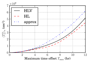
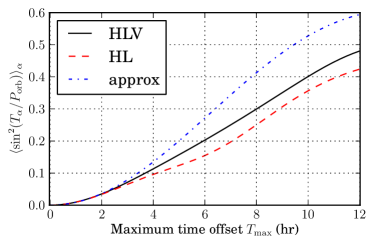
Figure 3: Plot of weighted averages $\left\langle\Delta t_{\alpha}^{2}\right\rangle_{\!\alpha}$ and $\left\langle\sin^{2}\frac{\pi\Delta t_{\alpha}}{P_{\text{orb}}}\right\rangle_{\!\alpha}$ appearing in the metric components (98) as a function of maximum allowed lag time $T_{\text{max}}$. The dotted lines show the approximate values (100) and (101) neglecting the variation of the weighting factor. The solid line (labeled HLV) shows the value for a search using detectors at the LIGO Hanford, LIGO Livingston, and Virgo sites, assuming a source at the sky position of Sco X-1, and that all detectors have the same sensitivity at the relevant frequency, and all sidereal times are evenly sampled. The dashed line (HL) shows the same thing for a search using only the LIGO detectors at Hanford and Livingston. The actual weighted averages (and therefore the number of templates needed to cover the parameter space) are less than the approximate ones, because the geometrical factor $(\Gamma^{\text{ave}}_{\alpha})^{2}$ weights smaller lag times more.

Note that some care needs to be taken when comparing our metric expressions to those in Leaci and Prix (2015). For example, combining (98a) with (100) gives us $g_{f_{0}f_{0}}\approx 2\pi^{2}\frac{T_{\text{max}}^{2}}{3}$, which seems at odds with the analogous expression in e.g., Eq. (61) of Leaci and Prix (2015), where the corresponding metric element is $\pi^{2}\frac{(\Delta{T})^{2}}{3}$. The difference is that the semicoherent search in Leaci and Prix (2015) is defined by combining distinct coherent segments of length $\Delta{T}$, which makes the mean squared difference

$$\frac{1}{(\Delta{T})^{2}}\int_{0}^{\Delta{T}}\int_{0}^{\Delta{T}}(t-t^{\prime})^{2}\,dt\,dt^{\prime}\\ =\frac{1}{(\Delta{T})^{2}}\int_{-\Delta{T}}^{\Delta{T}}\int_{\left\lvert\Delta{t}\right\rvert/2}^{\Delta{T}-\left\lvert\Delta{t}\right\rvert/2}(\Delta{t})^{2}\,d\overline{t}\,d\Delta{t}\\ =\frac{1}{(\Delta{T})^{2}}\int_{-\Delta{T}}^{\Delta{T}}(\Delta{t})^{2}(\Delta{T}-\left\lvert\Delta{t}\right\rvert)\,d\Delta{t}\\ =\left(\frac{2}{3}-\frac{2}{4}\right)(\Delta{T})^{2}=\frac{1}{6}(\Delta{T})^{2}$$ (102)

whereas our maximum lag rule $\left\lvert t-t^{\prime}\right\rvert<T_{\text{max}}$ gives a mean square time difference

$$\frac{\int_{0}^{T_{\text{obs}}}\int_{\max(t^{\prime}-T_{\text{max}},0)}^{\min(t^{\prime}+T_{\text{max}},T_{\text{obs}})}(t-t^{\prime})^{2}\,dt\,dt^{\prime}}{\int_{0}^{T_{\text{obs}}}\int_{\max(t^{\prime}-T_{\text{max}},0)}^{\min(t^{\prime}+T_{\text{max}},T_{\text{obs}})}dt\,dt^{\prime}}\\ =\frac{\int_{-\Delta{T}}^{\Delta{T}}\int_{\left\lvert\Delta{t}\right\rvert/2}^{T_{\text{obs}}-\left\lvert\Delta{t}\right\rvert/2}(\Delta{t})^{2}\,d\overline{t}\,d\Delta{t}}{\int_{-\Delta{T}}^{\Delta{T}}\int_{\left\lvert\Delta{t}\right\rvert/2}^{T_{\text{obs}}-\left\lvert\Delta{t}\right\rvert/2}d\overline{t}\,d\Delta{t}}\\ =\frac{(2/3)T_{\text{obs}}T_{\text{max}}^{3}-(2/4)T_{\text{max}}^{4}}{2T_{\text{obs}}T_{\text{max}}-T_{\text{max}}^{2}}\approx\frac{1}{3}T_{\text{max}}^{2}$$ (103)

where the assumption $T_{\text{max}}\ll T_{\text{obs}}$ gives us the result (100).

V Implications of deviation from signal model

So far, we have assumed that the underlying signal model contained in (21), along with the phase evolution (82) is correct, although some of the parameters may be unknown. We consider two effects which violate this assumption, and their potential impacts on the expected SNR (55). These are (1) spin wandering, in which the frequency is not a constant $f_{0}$ but varies slowly and unpredictably with time and (2) the impact of higher terms in the Taylor expansion of $\Phi(\mathfrak{t}(t))$ about $t=t_{K}$, which are neglected in the linear phase model (15). The former effect will place a potential limit on the coherence time $T_{\text{max}}$ by providing an intrinsic limit to the frequency resolution, whereas the latter will constrain our choice of SFT length $T_{\text{sft}}$ in order that neglected phase acceleration effects not cause too much loss of SNR.

V.1 Spin wandering

We have assumed so far that the LMXB is in approximate equilibrium, where the spin-up torque due to accretion is balanced by the spin-down due to gravitational waves. Even if this is true on average, the balance will not be perfect, and the spin frequency will “wander”. This means that rather than a constant frequency $f_{0}$ appearing in (82), there will be a time-varying frequency $f(\mathfrak{t})$, where $\mathfrak{t}=t-\frac{\vec{r}_{\text{det}}\cdot\hat{k}}{c}+\frac{\vec{r}_{\text{orb}}\cdot\hat{k}}{c}$ is the time measured in the neutron star’s rest frame. Thus the phase difference between SFTs $K$ and $L$ will be, rather than just $\Delta\Phi_{KL}=2\pi f_{0}[\mathfrak{t}_{K}-\mathfrak{t}_{L}]$,

$$\Delta\Phi_{KL}^{\text{true}}=\Phi_{K}-\Phi_{L}=2\pi\int_{\mathfrak{t}_{K}}^{\mathfrak{t}_{L}}f(\mathfrak{t})\,d\mathfrak{t}$$ (104)

We can consider the loss of SNR due to the existence of spin wandering, compared to what we would expect if the frequency truly were constant. Qualitatively, there are two reasons for loss of SNR: first, on short time scales, the change in frequency could disrupt the coherence between the two SFTs in a pair being cross correlated; second, on longer time scales, the spin could wander enough that the SNR is distributed over different frequency templates.

To quantify the loss of SNR we follow a calculation analogous to that in Sec. IV, e.g., in (68) and (69), to obtain

$$\frac{E\left[\rho\right]^{\text{ideal}}-E\left[\rho\right]}{E\left[\rho\right]^{\text{ideal}}}\approx\frac{1}{2}\left\langle\left(\Delta\Phi_{\alpha}^{\text{true}}-\Delta\Phi_{\alpha})\right)^{2}\right\rangle_{\alpha}$$ (105)

where $\langle\cdot\rangle_{\alpha}$ is a weighted average over SFT pairs with weighting factor $\left(\widehat{\Gamma}^{\text{ave}}_{\alpha}\right)^{2}$ as before. To estimate $\left\langle\left(\Delta\Phi_{\alpha}^{\text{true}}-\Delta\Phi_{\alpha})\right)^{2}\right\rangle_{\alpha}$ we assume that the wandering is slow enough that we can expand $f(\mathfrak{t})$ in a Taylor series about $\overline{\mathfrak{t}}_{KL}=(\mathfrak{t}_{K}+\mathfrak{t}_{L})/2$:

$$f(\mathfrak{t})\approx f(\overline{\mathfrak{t}}_{KL})+\dot{f}(\overline{\mathfrak{t}}_{KL})(\mathfrak{t}-\overline{\mathfrak{t}}_{KL})\\ \min(\mathfrak{t}_{K},\mathfrak{t}_{L})\leq\mathfrak{t}\leq\max(\mathfrak{t}_{K},\mathfrak{t}_{L})$$ (106)

Then

$$\Delta\Phi_{KL}^{\text{true}}-\Delta\Phi_{KL}=2\pi\int_{\mathfrak{t}_{K}}^{\mathfrak{t}_{L}}[f(\mathfrak{t})-f_{0}]\,d\mathfrak{t}\\ \approx 2\pi\left([f(\overline{\mathfrak{t}}_{KL})-f_{0}]\Delta\mathfrak{t}_{KL}+\dot{f}(\overline{\mathfrak{t}}_{KL})\frac{(\Delta\mathfrak{t}_{KL})^{2}}{2}\right)\ ,$$ (107)

where $\Delta\mathfrak{t}_{KL}=\mathfrak{t}_{K}-\mathfrak{t}_{L}$ Subject to reasonable assumptions about the randomness of the spin wandering, (105) can be written in the form

$$\begin{split}\frac{E\left[\rho\right]^{\text{ideal}}-E\left[\rho\right]}{E\left[\rho\right]^{\text{ideal}}}\approx&\ 2\pi^{2}\left\langle[f(\overline{\mathfrak{t}}_{\alpha})-f_{0}]^{2}\right\rangle_{\alpha}\left\langle(\Delta\mathfrak{t}_{\alpha})^{2}\right\rangle_{\alpha}\\ &+\frac{\pi^{2}}{2}\left\langle[\dot{f}(\overline{\mathfrak{t}}_{\alpha})]^{2}\right\rangle_{\alpha}\left\langle(\Delta\mathfrak{t}_{\alpha})^{4}\right\rangle_{\alpha}\\ \approx&\ 2\pi^{2}\left\langle[f(\overline{t}_{\alpha})-f_{0}]^{2}\right\rangle_{\alpha}\left\langle(\Delta t_{\alpha})^{2}\right\rangle_{\alpha}\\ &+\frac{\pi^{2}}{2}\left\langle[\dot{f}(\overline{t}_{\alpha})]^{2}\right\rangle_{\alpha}\left\langle(\Delta t_{\alpha})^{4}\right\rangle_{\alpha}\end{split}$$ (108)

where in the last expression we have used the fact that since $a_{p}$ and $\Delta d_{\alpha}$ are small, $\left\lvert\mathfrak{t}_{K}-t_{K}\right\rvert\ll T_{\text{max}}$. The two terms in (108) quantify the effects we predicted at the beginning of the section. The second term describes a loss of SNR due to the neutron star spin not being constant during the time spanned by a SFT pair, while the first term indicates a loss due to the mismatch between contributing frequencies and the frequency of a single template. [In fact, the first term is just $g_{f_{0}f_{0}}\left\langle[f(\overline{t}_{\alpha})-f_{0}]^{2}\right\rangle_{\alpha}$.[ Note that we are free to choose the $f_{0}$ which maximizes the SNR for a given instantiation of spin wandering, which will be $f_{0}=\left\langle f(\overline{t}_{\alpha})\right\rangle_{\alpha}$, so

$$\left\langle[f(\overline{t}_{\alpha})-f_{0}]^{2}\right\rangle_{\alpha}=\left\langle[f(\overline{t}_{\alpha})-\langle f(\overline{t}_{\alpha})\rangle_{\alpha}]^{2}\right\rangle_{\alpha}$$ (109)

is the weighted variance of $f(t)$ over the observing time.

To get a quantitative estimate of the effects of spin wandering, consider a model where the neutron star spins up or down linearly with typical amplitude $\lvert\dot{f}\rvert_{\text{drift}}$, changing on a time scale $T_{\text{drift}}$ where $T_{\text{max}}\ll T_{\text{drift}}\ll T_{\text{obs}}$. For simplicity, also neglect the impact of the weighting factor $\left(\widehat{\Gamma}^{\text{ave}}_{\alpha}\right)^{2}$, so that $\langle\Delta t_{\alpha}^{2}\rangle\approx\frac{T_{\text{max}}^{2}}{3}$ and $\langle\Delta t_{\alpha}^{4}\rangle\approx\frac{T_{\text{max}}^{4}}{5}$. Then

$$\left\langle[\dot{f}(\overline{t}_{\alpha})]^{2}\right\rangle_{\alpha}\lesssim\lvert\dot{f}\rvert_{\text{drift}}^{2}$$ (110)

and

$$\begin{split}\left\langle[f(\overline{t}_{\alpha})-\langle f(\overline{t}_{\alpha})\rangle_{\alpha}]^{2}\right\rangle_{\alpha}&\lesssim\left\langle\left\lvert\frac{\overline{t}_{\alpha}-T_{\text{mid}}}{T_{\text{drift}}}\right\rvert\left(T_{\text{drift}}\lvert\dot{f}\rvert_{\text{drift}}\right)^{2}\right\rangle_{\alpha}\\ &\approx\frac{T_{\text{obs}}T_{\text{drift}}}{4}\lvert\dot{f}\rvert_{\text{drift}}^{2}\end{split}$$ (111)

Combining these results, we have

$$\frac{E\left[\rho\right]^{\text{ideal}}-E\left[\rho\right]}{E\left[\rho\right]^{\text{ideal}}}\lesssim\frac{\pi^{2}}{6}T_{\text{obs}}T_{\text{drift}}\lvert\dot{f}\rvert_{\text{drift}}^{2}T_{\text{max}}^{2}+\frac{\pi^{2}}{10}\lvert\dot{f}\rvert_{\text{drift}}^{2}T_{\text{max}}^{4}$$ (112)

So, in order to avoid a fractional loss in SNR of more than $\mu$, one would need to limit the lag time to

$$T_{\text{max}}\leq\min\left(\frac{\sqrt{6\mu}}{\pi}\left(\lvert\dot{f}\rvert_{\text{drift}}\sqrt{T_{\text{obs}}T_{\text{drift}}}\right)^{-1},\sqrt{\frac{\sqrt{10\mu}}{\pi}}\lvert\dot{f}\rvert_{\text{drift}}^{-1/2}\right)$$ (113)

For example, if $\lvert\dot{f}\rvert_{\text{drift}}=10^{-12}\text{\,Hz/s}$, $T_{\text{drift}}=10^{6}\text{\,s}$, $T_{\text{obs}}=1\text{\,Yr}$, and $\mu=0.1$, the first limit is about $44,\!000\text{\,s}$ and the second is $320,\!000\text{\,s}$. So in that case spin wandering would become an issue if $T_{\text{max}}\gtrsim 12\text{\,hr}$.

Note that this is somewhat less than the estimate $\Delta{T}\lesssim 3\text{\,day}$ given in Leaci and Prix (2015). The source of this apparent discrepancy is a combination of the distinction between the coherent segment length $\Delta{T}$ and the maximum lag time $T_{\text{max}}$, described in Sec. IV.2.3, and the rough nature of some estimates used in Leaci and Prix (2015). That work compares the change in frequency $\lvert\dot{f}\rvert_{\text{drift}}\sqrt{T_{\text{obs}}T_{\text{drift}}/2}$ to the frequency resolution, which they give as $\sim 1/\Delta{T}$. This is effectively an order of magnitude estimate, since it effectively assumes $\mu=1$, and also leaves out the numerical factor in $1/\sqrt{g_{f_{0}f_{0}}}=\sqrt{3}/(\pi\Delta{T})$. On the other hand, their frequency drift is the expected drift from the middle of the run to the end; averaging the drift over the run gives an effective change of $(\lvert\dot{f}\rvert_{\text{drift}}\sqrt{T_{\text{obs}}T_{\text{drift}}})/2$. Including these three effects to do a calculation analogous to the one here would give a factor of $\pi\sqrt{5/3}\approx 4$ reduction on the estimated tolerable segment length to $\Delta{T}\lesssim 2\sqrt{3\mu}/\pi\left(\lvert\dot{f}\rvert_{\text{drift}}\sqrt{T_{\text{obs}}T_{\text{drift}}}\right)^{-1}\approx 62,\!000\text{\,s}\approx 17\text{\,hr}$. Of course, the assumptions of $\lvert\dot{f}\rvert_{\text{drift}}$ and $T_{\text{drift}}$ given above are uncertain and somewhat arbitrary, so our 12-hour number should also not be viewed as an exact constraint on the method.

V.2 SFT length

Most searches for continuous gravitational waves have used short Fourier transforms with a duration $T_{\text{sft}}$ of $30\text{\,min}=1800\text{\,s}$. The limiting factor which sets a maximum on the reasonable $T_{\text{sft}}$ is the accuracy of the linear phase approximation (15).

If we consider higher order terms in the phase expansion, we have

$$\Phi(\mathfrak{t}(t))\approx\Phi_{K}+2\pi f_{K}(t-t_{K})+\frac{1}{2}\ddot{\Phi}(t_{K})(t-t_{K})^{2}\\ +\frac{1}{3!}\dddot{\Phi}(t_{K})(t-t_{K})^{3}+\frac{1}{4!}\ddddot{\Phi}(t_{K})(t-t_{K})^{4}+\ldots\ .$$ (114)

The effect of these corrections is to modify (21) to

$$\widetilde{h}_{Kk}\approx h_{0}(-1)^{k}e^{\mathrm{i}\Phi_{K}}\frac{F^{K}_{+}\mathcal{A}_{+}-\mathrm{i}F^{K}_{\times}\mathcal{A}_{\times}}{2}\\ \times\int_{t_{K}-T_{\text{sft}}/2}^{t_{K}+T_{\text{sft}}/2}e^{-\mathrm{i}2\pi(f_{k}-f_{K})(t-t_{K})}\exp\left(\mathrm{i}\left[\frac{\ddot{\Phi}(t_{K})}{2}(t-t_{K})^{2}+\frac{\dddot{\Phi}(t_{K})}{3!}(t-t_{K})^{3}+\frac{\ddddot{\Phi}(t_{K})}{4!}(t-t_{K})^{4}\right]\right)dt\\ \approx h_{0}(-1)^{k}e^{\mathrm{i}\Phi_{K}}\frac{F^{K}_{+}\mathcal{A}_{+}-\mathrm{i}F^{K}_{\times}\mathcal{A}_{\times}}{2}T_{\text{sft}}\left[I_{0}(\kappa_{Kk})+i\frac{\ddot{\Phi}(t_{K})}{2}I_{2}(\kappa_{Kk})T_{\text{sft}}^{2}+i\frac{\dddot{\Phi}(t_{K})}{3!}I_{3}(\kappa_{Kk})T_{\text{sft}}^{3}\right.\\ \left.+\left(i\frac{\ddddot{\Phi}(t_{K})}{4!}-\frac{[\ddot{\Phi}(t_{K})]^{2}}{8}\right)I_{4}(\kappa_{Kk})T_{\text{sft}}^{4}\right]$$ (115)

where

$$I_{n}(\kappa)\equiv\int_{-1/2}^{1/2}x^{n}e^{-\mathrm{i}2\pi\kappa x}\,dx=\left(\frac{\mathrm{i}}{2\pi}\right)^{n}\frac{d^{n}}{d\kappa^{n}}\operatorname{sinc}(\kappa)$$ (116)

Note that for even $n$, $I_{n}(\kappa)$ is real and even, while for odd $n$, it is imaginary and odd.

We can then construct, as a replacement for (25),

$$\begin{split}\mu_{K}&=\frac{1}{\Xi_{K}}\sum_{k\in\mathcal{K}_{K}}(-1)^{k}I_{0}(\kappa_{Kk})\widetilde{h}_{Kk}\\ &\approx h_{0}e^{\mathrm{i}\Phi_{K}}\frac{F^{K}_{+}\mathcal{A}_{+}-\mathrm{i}F^{K}_{\times}\mathcal{A}_{\times}}{2}\frac{Q_{K}}{\Xi_{K}}\sqrt{\frac{2T_{\text{sft}}}{S_{K}}}\end{split}$$ (117)

where

$$\begin{split}Q_{K}=&\,\ \Xi_{K}^{2}+i\frac{\ddot{\Phi}(t_{K})}{2}\Sigma_{K02}\,T_{\text{sft}}^{2}+i\frac{\dddot{\Phi}(t_{K})}{3!}\Sigma_{K03}\,T_{\text{sft}}^{3}\\ &+\left(i\frac{\ddddot{\Phi}(t_{K})}{4!}-\frac{[\ddot{\Phi}(t_{K})]^{2}}{8}\right)\Sigma_{K04}\,T_{\text{sft}}^{4}\end{split}$$ (118)

and

$$\Sigma_{K0n}=\sum_{k\in\mathcal{K}_{K}}I_{0}(\kappa_{Kk})I_{n}(\kappa_{Kk})$$ (119)

The expectation value (43) of the statistic thus becomes, including the correction for higher phase derivatives and finite SFT length,

$$E\left[\rho\right]\approx Nh_{0}^{2}\,2\sum_{KL\in\mathcal{P}}\widehat{\Gamma}^{\text{ave}}_{KL}\operatorname{Re}\left(Q_{K}Q_{L}^{*}\widehat{\Gamma}_{KL}\right)$$ (120)

As in Sec. III.2 we assume that the sum over pairs evenly and independently samples the fractional frequency offset $\tilde{\kappa}_{K}$ from each SFT, which means we can replace $Q_{K}$ and $Q_{L}$ with

$$\begin{split}\langle Q_{K}\rangle_{\kappa}=&\ \langle\Xi^{2}\rangle+i\frac{\ddot{\Phi}(t_{K})}{2}\langle\Sigma_{02}\rangle\,T_{\text{sft}}^{2}\\ &+\left(i\frac{\ddddot{\Phi}(t_{K})}{4!}-\frac{[\ddot{\Phi}(t_{K})]^{2}}{8}\right)\langle\Sigma_{04}\rangle\,T_{\text{sft}}^{4}\end{split}$$ (121)

where the fact that $I_{3}(\kappa)$ is odd in $\kappa$ means that the average $\langle\Sigma_{03}\rangle$ vanishes.

Now,

$$\operatorname{Re}\left(Q_{K}Q_{L}^{*}\widehat{\Gamma}_{KL}\right)=\operatorname{Re}\left(Q_{K}Q_{L}^{*}\right)\operatorname{Re}\widehat{\Gamma}_{KL}-\operatorname{Im}\left(Q_{K}Q_{L}^{*}\right)\operatorname{Im}\widehat{\Gamma}_{KL}\\ \approx\operatorname{Re}\left(Q_{K}Q_{L}^{*}\right)\frac{5}{2}\frac{\mathcal{A}_{+}^{2}+\mathcal{A}_{\times}^{2}}{2}\widehat{\Gamma}^{\text{ave}}_{KL}-\operatorname{Im}\left(Q_{K}Q_{L}^{*}\right)\frac{5\mathcal{A}_{+}\mathcal{A}_{\times}}{2}\Gamma^{\text{circ}}_{KL}$$ (122)

We assume that the impact of the second piece is small and focus only on $\operatorname{Re}\left(Q_{K}Q_{L}^{*}\right)$, which leads to a fractional loss of SNR of

$$1-\frac{E\left[\rho\right]}{E\left[\rho\right]_{\text{ideal}}}=\frac{\langle\Xi^{2}\rangle^{2}-\langle\operatorname{Re}\left(Q_{K}Q_{L}^{*}\right)\rangle}{\langle\Xi^{2}\rangle^{2}}\\ =\left(\frac{\langle\ddot{\Phi}_{K}^{2}\rangle+\langle\ddot{\Phi}_{L}^{2}\rangle}{8}\frac{\langle\Sigma_{04}\rangle}{\langle\Xi^{2}\rangle}-\frac{\langle\ddot{\Phi}_{K}\ddot{\Phi}_{L}\rangle}{4}\frac{\langle\Sigma_{02}\rangle^{2}}{\langle\Xi^{2}\rangle^{2}}\right)T_{\text{sft}}^{4}$$ (123)

Differentiating (82) gives

$$\ddot{\Phi}_{K}=2\pi f_{0}\ddot{d}_{K}-\frac{(2\pi)^{3}}{P_{\text{orb}}^{2}}f_{0}a_{p}\sin\left[\frac{2\pi}{P_{\text{orb}}}(t_{K}-t_{\text{asc}})\right]$$ (124)

We can neglect the first term, since the acceleration due to the Earth’s orbit is $\mathcal{O}(10^{-11}\text{\,s}^{-1})$ and that due to the Earth’s rotation is $\mathcal{O}(10^{-10}\text{\,s}^{-1})$. In comparison, for Sco X-1,

$$a_{p}\left(\frac{2\pi}{P_{\text{orb}}}\right)^{2}=1.23\times 10^{-8}\text{\,s}^{-1}$$ (125)

If we assume, as in the metric calculation, that the average over pairs evenly samples the orbital phase, then

$$\langle\ddot{\Phi}_{K}^{2}\rangle+\langle\ddot{\Phi}_{L}^{2}\rangle=\frac{(2\pi)^{6}f_{0}^{2}a_{p}^{2}}{P_{\text{orb}}^{4}}$$ (126)

Using the identity

$$\sin A\sin B=\frac{1}{2}\left[\cos(A-B)-\cos(A+B)\right]$$ (127)

we can calculate

$$\left\langle\sin\left[\frac{2\pi}{P_{\text{orb}}}(t_{K}-t_{\text{asc}})\right]\sin\left[\frac{2\pi}{P_{\text{orb}}}(t_{L}-t_{\text{asc}})\right]\right\rangle\\ =\frac{1}{2}\left(\left\langle\cos\frac{2\pi\Delta t_{\alpha}}{P_{\text{orb}}}\right\rangle_{\!\alpha}-\left\langle\cos\frac{4\pi(\overline{t}_{\alpha}-t_{\text{asc}})}{P_{\text{orb}}}\right\rangle_{\!\alpha}\right)$$ (128)

so the fractional loss in SNR is

$$1-\frac{E\left[\rho\right]}{E\left[\rho\right]_{\text{ideal}}}\\ \approx\frac{8\pi^{6}f_{0}^{2}a_{p}^{2}}{P_{\text{orb}}^{4}}\left(\frac{\langle\Sigma_{04}\rangle}{\langle\Xi^{2}\rangle}-\frac{\langle\Sigma_{02}\rangle^{2}}{\langle\Xi^{2}\rangle^{2}}\left\langle\cos\frac{2\pi\Delta t_{\alpha}}{P_{\text{orb}}}\right\rangle_{\!\alpha}\right)T_{\text{sft}}^{4}$$ (129)

The factors $\langle\Sigma_{04}\rangle$ and $\langle\Sigma_{02}\rangle$ can be calculated by using (119) along with

$$I_{2}(\kappa)=\frac{\sin\pi\kappa}{4\pi\kappa}+\frac{\cos\pi\kappa}{2(\pi\kappa)^{2}}-\frac{\sin\pi\kappa}{2(\pi\kappa)^{3}}$$ (130)

and

$$I_{4}(\kappa)=\frac{\sin\pi\kappa}{16\pi\kappa}+\frac{\cos\pi\kappa}{4(\pi\kappa)^{2}}-\frac{3\sin\pi\kappa}{4(\pi\kappa)^{3}}-\frac{3\cos\pi\kappa}{2(\pi\kappa)^{4}}+\frac{3\sin\pi\kappa}{2(\pi\kappa)^{5}}$$ (131)

and averaging numerically over $\kappa$ given the number of frequency bins included. In Table 4, we show the two coefficients appearing in (129), for various choices of the number $m$ of included frequency bins (see also Table 2).

Table 4: The coefficients $\langle\Sigma_{04}\rangle/\langle\Xi^{2}\rangle$ and $\langle\Sigma_{02}\rangle^{2}/\langle\Xi^{2}\rangle^{2}$ appearing in (129), for various choices of the number $m$ of included frequency bins, where $\langle\Sigma_{0n}\rangle$ is the mean value of $\Sigma_{0n}(\kappa)=\sum_{s=-\left\lceil(m-1)/2\right\rceil}^{\left\lfloor(m-1)/2\right\rfloor}I_{0}(\kappa+s)I_{n}(\kappa+s)$, averaged over $-\frac{1}{2}\leq\kappa\leq\frac{1}{2}$, and $I_{n}(\kappa)$ is defined in (116) with $I_{0}(\kappa)=\operatorname{sinc}\kappa=\frac{\sin\pi\kappa}{\pi\kappa}$, and $I_{2}(\kappa)$ and $I_{4}(\kappa)$ are given by (130) and (131). Note that the value of $\langle\Xi^{2}\rangle\equiv\langle I_{00}\rangle$ is tabulated in Table 2.

$m$	1	2	3	4	5	6
$\langle\Sigma_{04}\rangle/\langle\Xi^{2}\rangle$	0.0107	0.0086	0.0099	0.0100	0.0106	0.0108
$\langle\Sigma_{02}\rangle^{2}/\langle\Xi^{2}\rangle^{2}$	0.0056	0.0042	0.0052	0.0055	0.0059	0.0060

Note that for the cross-correlation search, choosing shorter SFTs does not directly impact the sensitivity. For the same allowed lag time, searches with different SFT lengths should have approximately the same sensitivity. We can see this by considering the SNR for a given signal amplitude $h_{0}$, for example, from (52). Since

$$\widehat{\Gamma}^{\text{ave}}_{KL}=\Gamma_{KL}\frac{2T_{\text{sft}}}{\sqrt{S_{K}S_{L}}}$$ (132)

the quantity $(\widehat{\Gamma}^{\text{ave}}_{KL})^{2}$ inside the sum is proportional to $(T_{\text{sft}})^{2}$. However, for a fixed maximum time lag $T_{\text{max}}$, the number of terms in the sum will be proportional to $(T_{\text{sft}})^{-2}$ and the resulting expected SNR will be approximately independent of $T_{\text{sft}}$. (For example, halving the SFT length will mean each SFT pair contributed one-fourth as much to the sensitivity, but will double the number of SFTs and thus quadruple the number of SFT pairs.)

On the other hand, by increasing the number of SFT pairs, using a shorter SFT length will mean increasing computing cost at the same $T_{\text{max}}$. If the computing budget is fixed, the sensitivity gained by reducing the mismatch (129) will be offset by the loss of sensitivity, in the form of a lower $E\left[\rho\right]_{\text{ideal}}$, resulting from a smaller $T_{\text{max}}$. Following the reasoning in Sec. III.2, if the computing cost scales like the number of templates (which scales like $T_{\text{max}}^{d}$) times the number of SFT pairs (which scales like $T_{\text{max}}T_{\text{obs}}T_{\text{sft}}^{-2}$), then the overall sensitivity for a fixed observing time $T_{\text{obs}}$ scales like $T_{\text{max}}^{d+1}T_{\text{sft}}^{-2}$, and therefore the restriction at constant computing cost will be $T_{\text{max}}\propto T_{\text{sft}}^{\frac{2}{d+1}}$. Since the sensitivity scales with the square root of the number of SFT pairs, we have $E\left[\rho\right]^{\text{ideal}}\propto T_{\text{sft}}^{\frac{1}{d+1}}$ and

$$E\left[\rho\right]\propto T_{\text{sft}}^{\frac{1}{d+1}}\left(1-Af_{0}^{2}T_{\text{sft}}^{4}\right)$$ (133)

where

$$A\approx\frac{8\pi^{6}a_{p}^{2}}{P_{\text{orb}}^{4}}\left(\frac{\langle\Sigma_{04}\rangle}{\langle\Xi^{2}\rangle}-\frac{\langle\Sigma_{02}\rangle^{2}}{\langle\Xi^{2}\rangle^{2}}\left\langle\cos\frac{2\pi\Delta t_{\alpha}}{P_{\text{orb}}}\right\rangle_{\!\alpha}\right)$$ (134)

is the mismatch scaling appearing in (129). The sensitivity at fixed computing cost is thus maximized when

$$1-(4d+5)Af_{0}^{2}T_{\text{sft}}^{4}=0$$ (135)

i.e., when the mismatch due to SFT length is

$$\mu=Af_{0}^{2}T_{\text{sft}}^{4}=\mu^{\text{opt}}=\frac{1}{4d+5}$$ (136)

The corresponding optimal SFT length is

$$T_{\text{sft}}=([4d+5]A)^{-1/4}f_{0}^{-1/2}$$ (137)

For example, if $d=3$, $\mu^{\text{opt}}=\frac{1}{17}\approx 0.059$. In Fig. 4, we show this optimal SFT length for $d=3$, using $a_{p}=1.44\text{\,s}$ and $P_{\text{orb}}=68023.70\text{\,s}$ (the most likely values for Sco X-1). The solid line shows the most optimistic scenario, in which $\left\langle\cos\frac{2\pi\Delta t_{\!\alpha}}{P_{\text{orb}}}\right\rangle_{\alpha}\approx 1$ (which will be the case for $T_{\text{max}}\ll P_{\text{orb}}$) and the dashed line shows the most pessimistic scenario, in which the average goes to zero.

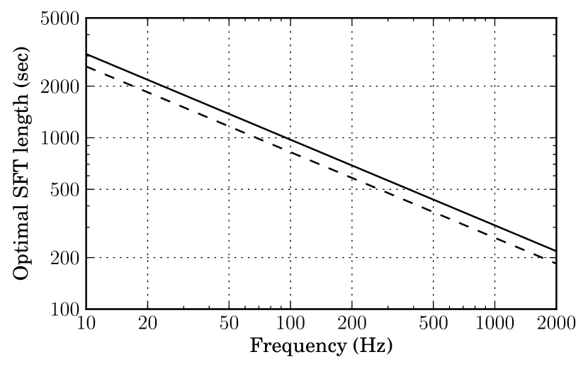
Figure 4: The optimal SFT length $T_{\text{sft}}$, defined in (137) and (134), as a function of frequency, for a signal with the most likely orbital parameters for Sco X-1, as given in Table 1, assuming that $d=3$, i.e., the density of points in parameter space grows as the third power of the coherence time $T_{\text{max}}$. This is appropriate for a search over, e.g., frequency $f_{0}$, projected semimajor axis $a_{p}$, and time of ascension $t_{\text{asc}}$ (when the uncertainty in the period $P_{\text{orb}}$ is small enough that a single value may be assumed), in the case where $T_{\text{max}}$ is small compared with $P_{\text{orb}}$. The solid line represents a more optimistic scenario where the average cosine appearing in the second term of (134) is approximately unity, which should also be the case if $T_{\text{max}}\ll P_{\text{orb}}$. The dashed line represents a worst-case scenario where the average is approximately zero. The optimal SFT length maximizes the expected SNR in (133) and represents a balance between two competing effects: if $T_{\text{sft}}$ is too large, phase acceleration will lead to a loss in SNR compared to the ideal formula (55); if $T_{\text{sft}}$ is too small, the large number of SFT pairs in the computation will lead to a restriction on the possible $T_{\text{max}}$ achievable at fixed computing cost, and reduce the ideal SNR itself.

VI Conclusions and outlook

In this paper we have explored details of the model-based cross-correlation search for periodic gravitational waves, focusing on its application to signals from neutron stars in binary systems (LMXBs) and Scorpius X-1 in particular. We have carefully considered the impact of spectral leakage (in Sec. III.2) and the implications of unknown amplitude parameters (in Sec. III.3) on the sensitivity of the method. We have also produced expressions for the parameter space metric of the search (in Sec. IV.2), at varying levels of approximation, and a systematic offset in the parameters of a detected signal related to the unmeasured inclination angle of the neutron star to the line of sight (in Sec. IV.1). In Sec. V.1 we estimated the effects of “spin wandering” caused by deviations from equilibrium in the torque balance configuration, and in (V.2) we consider the appropriate SFT duration needed to avoid significant loss of SNR due to unmodeled phase acceleration.

We have shown (in Sec. III.4) that the method produces an improvement in strain sensitivity over the directed stochastic search method which inspired it; this is roughly proportional to the fourth root of the product of the coherence time of the model-based search and the frequency bin size for the stochastic search. A mock data challenge Messenger et al. (2015) has been carried out by comparing the performance of the available search methods, including the model-based cross-correlation search, on simulated signals injected into Gaussian noise. As reported elsewhere Messenger et al. (2015); Zhang et al. (2015), the cross-correlation search is the most sensitive one currently implemented.

To give an estimate of expected sensitivity for data from detectors such as Advanced LIGO and Advanced Virgo, it is necessary to make some suppositions about the parameters of the search, especially the time $T_{\text{max}}$ over which SFTs are coherently cross correlated. Since this drives both the sensitivity and computing cost, the choice of $T_{\text{max}}$ will depend on available computing resources, and will likely vary with frequency in order to optimize the distribution of computing resources where they can be most effective. In Zhang et al. (2015), we performed searches with $9\text{\,min}\leq T_{\text{max}}\leq 90\text{\,min}$ for a range of frequency bands covering a total of $500\text{\,Hz}$ distributed in $f_{0}\in[50,1455]\text{\,Hz}$, using moderate computational resources. On the other hand, in Sec. V.1, we considered spin wandering effects which might lead to a significant loss of SNR for a search with $T_{\text{max}}\gtrsim 12\text{\,hr}$ for a one-year observation.

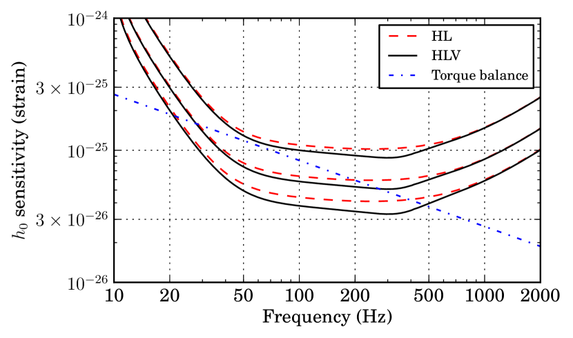
Figure 5: Expected sensitivity (61) for a search of one year of coincident data from either the two LIGO detectors (labeled HL) or the three LIGO+Virgo detectors (labeled HLV), at design sensitivity. The value plotted is the observable $h_{0}$ at 5% false dismissal probability, assuming an overall false alarm probability of 5% and a trials factor of $10^{8}$ for a single-template false alarm probability of $5\times 10^{-10}$ (i.e., see Sec. III.3 and Table 3). The three curves in each set, are, from top to bottom, for $T_{\text{max}}=6\text{\,min}$, $60\text{\,min}$ and $10\text{\,hr}$. They are compared to the signal strength (139) predicted by the torque balance argumentBildsten (1998).

In Fig. 5, we show the projected sensitivity (61) of a search using one year of data, either from the two advanced LIGO detectors in Hanford, WA and Livingston, LA, or from the two advanced LIGO detectors plus the Virgo detector in Cascina, Italy, all operating at their projected design sensitivity. We show the sensitivity of three hypothetical searches, with $T_{\text{max}}=6\text{\,min}$, $60\text{\,min}$ or $600\text{\,min}=10\text{\,hr}$, and compare the observable $h_{0}$ (at a 5% false dismissal probability, assuming a single-template false alarm probability of $5\times 10^{-10}$, corresponding to an overall 5% false alarm probability and a trails factor of $10^{8}$, as described in Sec. III.3 and Table 3). For comparison, we show a representative signal strength predicted by the torque balance argumentBildsten (1998); Watts et al. (2008). By assuming that the spin-down torque due to gravitational waves is balanced by the spin-up torque due to accretion, estimated using the observed x-ray flux, it is possible to estimate the strength of the gravitational-wave signal as a function of the neutron star spin frequency $\nu_{s}$Watts et al. (2008):

$$\begin{split}h_{0}\approx&\ 3\times 10^{-27}\left(\frac{F_{X}}{10^{-8}\text{\,erg}\text{\,cm}^{-2}\text{\,s}^{-1}}\right)^{1/2}\left(\frac{\nu_{s}}{300\text{\,Hz}}\right)^{-1/2}\\ &\times\left(\frac{R}{10\text{\,km}}\right)^{3/4}\left(\frac{M}{1.4M_{\odot}}\right)^{-1/4}\end{split}$$ (138)

The spin frequency of Sco X-1 is unknown, but $\nu_{s}$ values inferred for other LMXBs from pulsations or burst oscillations range from $50\text{\,Hz}$ to $600\text{\,Hz}$, so we consider the sensitivity over a wide range of GW frequencies. For Sco X-1, using the observed x-ray flux $F_{X}=3.9\times 10^{-7}\text{\,erg}\text{\,cm}^{-2}\text{\,s}^{-1}$ from Watts et al. (2008), and assuming that the GW frequency $f_{0}$ is twice the spin frequency $\nu_{s}$ (as would be the case for GWs generated by anisotropies in the neutron star), the torque balance value is

$$h_{0}\approx 3.4\times 10^{-26}\left(\frac{\nu_{s}}{300\text{\,Hz}}\right)^{-1/2}\ ,$$ (139)

which is the reference curve plotted in Fig. 5.

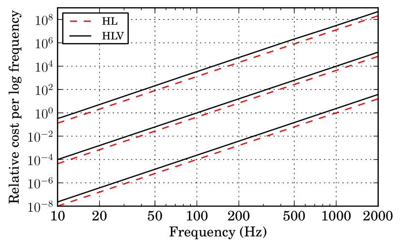
Figure 6: Relative scaling of expected computing cost per logarithmic frequency interval for a search of one year of coincident data from either the two LIGO detectors (labeled HL) or the three LIGO+Virgo detectors (labeled HLV). The three curves in each set, are, from top to bottom, for $T_{\text{max}}=10\text{\,hr}$, $60\text{\,min}$ and $6\text{\,min}$. The calculation assumes that the computing cost scales with the number of SFT pairs times the number of points in parameter space. It also assumes that the optimal SFT length $T_{\text{sft}}$ given by (137) and (134) has been chosen at each frequency, and that we are searching over frequency and two orbital parameters. The approximate scaling is as $f_{0}^{4}T_{\text{max}}^{4}$, so for instance a $T_{\text{max}}=60\text{\,min}$ search from $100$ to $200\text{\,Hz}$ would consume the same resources as a $T_{\text{max}}=6\text{\,min}$ search from $1000$ to $2000\text{\,Hz}$. For reference, the mock data analysis in Zhang et al. (2015), which was accomplished in approximately $20,\!000$ CPU-days, covered a set of roughly logarithmically-spaced frequency bands totaling $250\text{\,Hz}$ spread from $50\text{\,Hz}$ to $1375\text{\,Hz}$ at a range of $T_{\text{max}}$ values from $9$ to $90\text{\,min}$.

We see that for a three-detector, one-year analysis, a signal at the torque balance limit should be detectable for $30\text{\,Hz}\lesssim f_{0}\lesssim 300\text{\,Hz}$ with $T_{\text{max}}=60\text{\,min}$ (which is already computationally manageable at most frequencies), and if one could increase to $T_{\text{max}}=600\text{\,min}$ through algorithmic improvements, programming optimization, and/or application of additional resources, that range could be broadened to $20\text{\,Hz}\lesssim f_{0}\lesssim 500\text{\,Hz}$. The best-case $h_{0}$ sensitivity of $5\times 10^{-26}$ for the $60$ min search is consistent with the results of the Sco X-1 MDC Zhang et al. (2015); Messenger et al. (2015), where a cross-correlation search with $9\text{\,min}\leq T_{\text{max}}\leq 90\text{\,min}$ was able to detect signals with $h_{0}\gtrsim 5\times 10^{-26}$.

The choice of $T_{\text{max}}$ will in part be constrained by computing cost; in Fig. 6 we show the approximate relative computing cost scaling for the six searches considered (one year of data from either the two LIGO detectors or the two LIGO detectors and Virgo, with a maximum allowed lag time of $T_{\text{max}}=6\text{\,min}$, $60\text{\,min}$ or $600\text{\,min}=10\text{\,hr}$. The computing cost is assumed to be proportional to the number of SFT pairs times the number of parameter space points to be searched, and we plot the relative cost per logarithmic frequency interval. We also assume that at each frequency the SFT length is chosen to be the optimal SFT length given by (137) and (134). Roughly speaking, the number of SFT pairs will scale as $f_{0}T_{\text{max}}$ (since the optimal SFT length scales as $T_{\text{max}}^{-1/2}$), and the density of templates in parameter space will scale as $f_{0}^{2}T_{\text{max}}^{3}$. The density of points per logarithmic frequency interval introduces another factor of $f_{0}$, so the quantity plotted, cost per unit frequency interval, scales approximately as $f_{0}^{4}T_{\text{max}}^{4}$. This means that, for example, a $T_{\text{max}}=60\text{\,min}$ search from $100$ to $200\text{\,Hz}$ would consume the same resources as a $T_{\text{max}}=6\text{\,min}$ search from $1000$ to $2000\text{\,Hz}$ or a $T_{\text{max}}=600\text{\,min}$ search from $10$ to $20\text{\,Hz}$.

Finally, we consider one possible avenue for enhancement of the cross-correlation method. As explained in Sec. III.1, the fact that we filter with $G^{\text{ave}}_{KL}$ means that the method provides an estimate of $h_{0}^{\text{eff}}$, a function of $h_{0}$ and $\cos\iota$ defined in (46), rather than $h_{0}$. If we had a method of independently estimating $\cos\iota$, or in fact any other combination of $h_{0}$ and $\cos\iota$ besides $h_{0}^{\text{eff}}$, we could obtain a better measurement of $h_{0}$. In Dhurandhar et al. (2008), a method was proposed to obtain estimates of $h_{0}\mathcal{A}_{+}$ and $h_{0}\mathcal{A}_{\times}$, but a more effective procedure would seem to be adding a second statistic which uses $\mathrm{i}\Gamma^{\text{circ}}_{KL}$ [see (32b)] in place of $\Gamma^{\text{ave}}_{KL}$ and therefore observes the quantity $h_{0}^{2}\mathcal{A}_{+}\mathcal{A}_{\times}$; between this and the original $h_{0}^{\text{eff}}$ estimate, we would be able to disentangle $h_{0}$ and $\cos\iota$. This prospect bears further investigation.

Appendix A Effects of Nontrivial Windowing

A.1 General formulation

As noted in Sec. II.1, the construction of Fourier transformed data is often done with a window function $w(\theta)$, as in (3), as opposed to the unwindowed (or nearly-rectangularly-windowed) data considered in the main body of the text. This appendix considers the impact on the search method and its sensitivity of using a nontrivial window function, which is investigated in greater detail in Sundaresan and Whelan (2012).

The use of windowing for Fourier transforms affects the expected signal and noise contributions to the data. For the signal contribution, Eq. (16) becomes

$$\widetilde{h}_{Kk}\approx h_{0}(-1)^{k}e^{\mathrm{i}\Phi_{K}}\frac{F^{K}_{+}\mathcal{A}_{+}-\mathrm{i}F^{K}_{\times}\mathcal{A}_{\times}}{2}\delta^{w}_{T_{\text{sft}}}(f_{k}-f_{K})$$ (140)

where $\delta^{w}_{T_{\text{sft}}}(f_{k}-f_{K})$ is the generalization of the finite time delta function defined in (17):

$$\delta^{w}_{T_{\text{sft}}}(f_{k}-f_{K})\\ =\int_{t_{K}-T_{\text{sft}}/2}^{t_{K}+T_{\text{sft}}/2}w\left(\frac{t-t_{K}}{T_{\text{sft}}}\right)\,e^{-\mathrm{i}2\pi(f_{k}-f_{K})(t-t_{K})}\,dt\\ =T_{\text{sft}}\int_{1/2}^{1/2}w(\theta)\,e^{-\mathrm{i}2\pi\kappa_{Kk}\theta}\,d\theta\equiv T_{\text{sft}}\,\xi^{w}(\kappa_{Kk})$$ (141)

with $\kappa_{Kk}=(f_{k}-f_{K})T_{\text{sft}}$ as before. The noise contribution is modified by replacing (8) with

$$E\left[\widetilde{n}_{Kk}^{w}\widetilde{n}^{w*}_{L\ell}\right]\approx\delta_{KL}\,\gamma^{w}_{k\ell}\,T_{\text{sft}}\,\frac{S_{K}}{2}$$ (142)

where

$$\begin{split}\gamma^{w}_{k\ell}&=\frac{(-1)^{k-\ell}}{T_{\text{sft}}}\int_{-\infty}^{\infty}\delta^{w}_{T_{\text{sft}}}(f_{k}-f)\,\delta^{w*}_{T_{\text{sft}}}(f_{\ell}-f)\,df\\ &=(-1)^{k-\ell}\int_{-1/2}^{1/2}e^{\mathrm{i}2\pi(k-\ell)\theta}[w(\theta)]^{2}\,d\theta\end{split}$$ (143)

Note that the diagonal elements of this matrix are equal to the mean square of the window function:

$$\gamma^{w}_{kk}=\int_{-1/2}^{1/2}[w(\theta)]^{2}\,d\theta\equiv\overline{w^{2}}$$ (144)

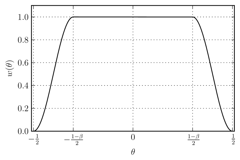
Figure 7: The general Tukey window $w_{\beta}(\theta)$ as defined in (151) for a generic value of the parameter $\beta\in[0,1]$, where $\beta$ is the fraction of the window length taken up by the transitions from $0$ to $1$ and back.

If we define

$$z^{w}_{K{k}}=\widetilde{x}^{w}_{K{k}}\sqrt{\frac{2}{T_{\text{sft}}S_{K}}}$$ (145)

as in (9), we have

$$E\left[z^{w}_{K{k}}\right]=\mu^{w}_{K{k}}\\ \approx h_{0}(-1)^{k}\xi^{w}(\kappa_{Kk})e^{\mathrm{i}\Phi_{K}}\frac{F^{K}_{+}\mathcal{A}_{+}-\mathrm{i}F^{K}_{\times}\mathcal{A}_{\times}}{2}\sqrt{\frac{2T_{\text{sft}}}{S_{K}}}$$ (146)

and

$$E\left[(z^{w}_{K{k}}-\mu^{w}_{K{k}})(z^{w}_{L{\ell}}-\mu^{w}_{L{\ell}})^{*}\right]=\delta_{KL}\,\gamma^{w}_{{k}{\ell}}\ .$$ (147)

We then modify (23) to

$$z^{w}_{K}\equiv\frac{1}{\Xi^{w}_{K}}\sum_{k\in\mathcal{K}_{K}}\sum_{k^{\prime}\in\mathcal{K}_{K}}(-1)^{k}\xi^{w*}\!(\kappa_{Kk})(\gamma^{w})^{-1}_{kk^{\prime}}\,z^{w}_{Kk^{\prime}}$$ (148)

where $\{(\gamma^{w})^{-1}_{k\ell}\}$ are the elements of the matrix inverse of $\{\gamma^{w}_{k\ell}\}$, and

$$\Xi^{w}_{K}=\sqrt{\sum_{k\in\mathcal{K}_{K}}\sum_{k^{\prime}\in\mathcal{K}_{K}}(-1)^{k-k^{\prime}}\xi^{w*}\!(\kappa_{Kk})\,(\gamma^{w})^{-1}_{kk^{\prime}}\,\xi^{w}(\kappa_{Kk^{\prime}})}$$ (149)

ensures that the normalization (24) holds as before. Then the derivation proceeds as before, with $\Xi^{w}_{K}$ replacing $\Xi_{K}$, and, in particular, the expected SNR (52) becomes

$$E\left[\rho\right]\approx(h^{\text{eff}}_{0})^{2}\langle(\Xi^{w})^{2}\rangle\sqrt{2\sum_{KL\in\mathcal{P}}\left(\widehat{\Gamma}^{\text{ave}}_{KL}\right)^{2}}$$ (150)

A.2 Results for specific windows

We now consider the consequences of the modification (150) by investigating the form of $\xi^{w}(\kappa)=T_{\text{sft}}^{-1}\delta^{w}_{T_{\text{sft}}}(\kappa/T_{\text{sft}})$ defined in (141) and $\gamma^{w}_{k\ell}$ defined in (143) for specific nonrectangular window choices. We consider the general family of Tukey windows, defined using an adjustable parameter $0\leq\beta\leq 1$ by

$$w_{\beta}(\theta)=\begin{cases}\frac{1}{2}\left(1-\cos\frac{\pi}{\beta}(2\theta+1)\right)&-\frac{1}{2}\leq\theta\leq-\left(\frac{1-\beta}{2}\right)\\ 1&-\left(\frac{1-\beta}{2}\right)\leq\theta\leq\left(\frac{1-\beta}{2}\right)\\ \frac{1}{2}\left(1-\cos\frac{\pi}{\beta}(2\theta-1)\right)&\left(\frac{1-\beta}{2}\right)\leq\theta\leq\frac{1}{2}\end{cases}\ .$$ (151)

The general form of the Tukey window is illustrated in Fig. 7. This family includes at its extremes the rectangular window ($\beta=0$) and the Hann window ($\beta=1$). In practical applications it is also common to use a Tukey window with a small finite parameter $\beta\ll 1$ rather than a pure rectangular window. These two specific cases are shown in Fig. 8, along with a Tukey window with $\beta=\frac{1}{2}$.

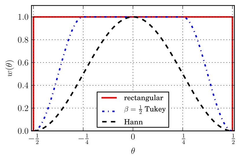
Figure 8: Specific versions of the general Tukey window $w_{\beta}(\theta)$ as defined in (151): the rectangular window $w^{\text{rect}}(\theta)=w_{0}(\theta)$, a canonical ($\beta=\frac{1}{2}$) Tukey window $w_{1/2}(\theta)$, and the Hann window $w^{\text{Hann}}(\theta)=w_{1}(\theta)$.

We can insert the general form of $w_{\beta}(\theta)$ from (151) into (141) to obtain

$$\xi^{w}_{\beta}(\kappa)=\frac{1}{2}\operatorname{sinc}\kappa+\frac{1}{2}(1-\beta)\operatorname{sinc}(\kappa[1-\beta])\\ +\frac{\beta}{4}\sin\left(\pi\kappa\left[1-\frac{\beta}{2}\right]\right)\left[\operatorname{sinc}\left(\frac{1-\beta\kappa}{2}\right)-\operatorname{sinc}\left(\frac{1+\beta\kappa}{2}\right)\right]\ ;$$ (152)

the “interesting” values of $\beta$ also have somewhat simpler explicit forms. For the rectangular window ($\beta=0$), which was considered in the main body of the paper, we have

$$\xi^{w}_{0}(\kappa)=\xi^{\text{rect}}(\kappa)=\operatorname{sinc}\kappa\ ;$$ (153)

for the Hann window ($\beta=1$), we have

$$\xi^{w}_{1}(\kappa)=\xi^{\text{Hann}}(\kappa)=\frac{1}{2}\operatorname{sinc}\kappa+\frac{1}{4}\operatorname{sinc}(1-\kappa)+\frac{1}{4}\operatorname{sinc}(1+\kappa)\ ;$$ (154)

and for the canonical ($\beta=\frac{1}{2}$) Tukey window, we have

$$\xi^{w}_{1/2}(\kappa)=\xi^{\text{Tukey}}(\kappa)\\ =\frac{1}{2}\operatorname{sinc}\kappa-\frac{1}{4}\operatorname{sinc}(2+\kappa)-\frac{1}{4}\operatorname{sinc}(2-\kappa)\\ +\frac{1}{4}\operatorname{sinc}\frac{\kappa}{2}+\frac{1}{8}\operatorname{sinc}\left(1+\frac{\kappa}{2}\right)+\frac{1}{8}\operatorname{sinc}\left(1-\frac{\kappa}{2}\right)$$ (155)

We plot these three functions in Fig. 9.

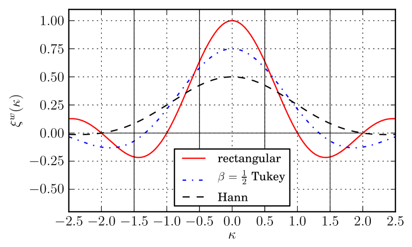
Figure 9: The window leakage function $\xi^{w}(\kappa)=T_{\text{sft}}^{-1}\delta^{w}_{T_{\text{sft}}}(\kappa/T_{\text{sft}})$ defined in (141) for the windows shown in Fig. 8. The explicit formulas are given in (153) for the rectangular window, (155) for the canonical ($\beta=\frac{1}{2}$) Tukey window, and (154) for the Hann window. Note that the version for rectangular-windowed data is just $\xi^{\text{rect}}(\kappa)=T_{\text{sft}}^{-1}\delta_{T_{\text{sft}}}(\kappa/T_{\text{sft}})=\operatorname{sinc}(\kappa)=\frac{\sin\pi\kappa}{\pi\kappa}$, which is the finite-time delta function plotted in Fig. 1.

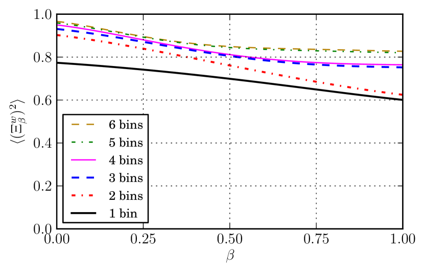
Figure 10: The leakage factor $\langle(\Xi^{w})^{2}\rangle$ appearing in (150) for a search using between one and six bins from each SFT, assuming a general Tukey window from the family (151). We see that, for any number of bins, the most sensitive search is when $\beta=0$, i.e., for rectangular windows. In particular, when a single bin is used from each SFT, we have $\langle\Xi^{2}\rangle=0.774$ for rectangular windowing ($\beta=0$), $\langle(\Xi^{w}_{\beta})^{2}\rangle=0.699$ for a canonical ($\beta=\frac{1}{2}$) Tukey window, and $\langle(\Xi^{\text{Hann}})^{2}\rangle=0.601$ for Hann windowing ($\beta=1$). Note that the $\beta=0$ value on each curve is just the corresponding “cumulative” number from Table 2.

To evaluate the factor of $\langle(\Xi^{w})^{2}\rangle$ appearing in (150), we need to construct the matrix $\{\gamma^{w}_{k\ell}\}$ via (143). Substituting (151) into (143), we can find

$$(\gamma^{w}_{\beta})_{k\ell}=(-1)^{k-\ell}(1-\beta)\operatorname{sinc}\left[(k-\ell)(1-\beta)\right]\\ +\frac{3}{8}\beta\operatorname{sinc}\left[(k-\ell)\beta\right]\\ -\frac{1}{4}\beta\operatorname{sinc}\left[(k-\ell)\beta-1\right]-\frac{1}{4}\beta\operatorname{sinc}\left[(k-\ell)\beta+1\right]\\ +\frac{1}{16}\beta\operatorname{sinc}\left[(k-\ell)\beta-2\right]+\frac{1}{16}\beta\operatorname{sinc}\left[(k-\ell)\beta+2\right]\ .$$ (156)

We can see that, for the rectangular case $\beta=0$, we get $(\gamma^{w}_{0})_{k\ell}=\delta_{k\ell}$ as before, while for the Hann case $\beta=1$ we have

$$\gamma^{\text{Hann}}_{k\ell}=\frac{3}{8}\delta_{k,\ell}-\frac{1}{4}\delta_{k,\ell-1}-\frac{1}{4}\delta_{k,\ell+1}+\frac{1}{16}\delta_{k,\ell-2}+\frac{1}{16}\delta_{k,\ell+2}\ .$$ (157)

The diagonal elements for general $\beta$ are

$$(\gamma^{w}_{\beta})_{kk}=1-\frac{5}{8}\beta=\overline{w^{2}_{\beta}}$$ (158)

as in (144). This means that, in the special case where the set of bins $\mathcal{K}_{K}$ from each SFT is just the “best bin” $\tilde{k}_{K}$ defined in (18), the matrix $\{\gamma^{w}_{k\ell}\}$ just has a single element $\gamma^{w}_{\tilde{k}_{K}\tilde{k}_{K}}=1-\frac{5}{8}\beta$, and

$$(\Xi^{w}_{K})^{2}=\frac{\left\lvert\xi^{w}_{\beta}(\tilde{\kappa}_{K})\right\rvert^{2}}{1-\frac{5}{8}\beta}$$ (159)

where $\xi^{w}_{\beta}(\kappa)$ is defined in (152). In general, though, we need to invert the matrix (156) and then average $(\Xi^{w}_{K})^{2}$ defined in (149) over possible values of $\tilde{\kappa}_{K}$. We plot the results in Fig. 10 as a function of $\beta$, for cases where we take the “best” $m$ bins from each SFT. We see that, for any number of bins, $\langle(\Xi^{w})^{2}\rangle$ is a maximum for $\beta=0$, i.e., rectangular windowing. The $\beta=0$ values are just the “cumulative” entries from Table 2 for the corresponding number of bins. Specifically, for the single-bin case, when $\beta=0$, we have $\langle\Xi^{2}\rangle=0.774$ (as seen in the $m=1$ entry of Table 2), when $\beta=\frac{1}{2}$, we have $\langle(\Xi^{\text{Tukey}})^{2}\rangle=0.699$, and when $\beta=1$, we have $\langle(\Xi^{\text{Hann}})^{2}\rangle=0.601$. These values also appear in Sundaresan and Whelan (2012), which explains in more detail the relevant phenomenon. While the dropoff from the maximum value of $(\Xi^{w}_{K})^{2}$ to its average value is greatest for rectangular windowing, the maximum value and the average value are also greatest for the rectangular window.

A common approach to handle the loss of signal associated with Hann-windowed data is to divide the data into overlapping Hann-windowed data segments, as in Goetz and Riles (2011). For the present search, however, it is easier just to include more bins from the rectangularly windowed Fourier transform, if desired, to increase the sensitivity of the search. The only drawback to that is a slight increase in computational time, but this increase is much smaller than what would arise from almost doubling the number of SFTs by the use of overlapping windows.

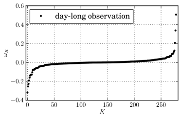
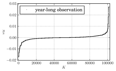
Figure 11: Eigenvalues $\{\omega_{K}\}$ of the weights matrix $\mathbf{W}$ defined in(35) for two scenarios. On the left, we show one day of observation with the LLO, LHO and Virgo detectors, assuming equal sensitivity, with $T_{\text{sft}}=900\text{\,s}$ and $T_{\text{max}}=3600\text{\,s}$. On the right, we show one year of observation under the same conditions, constructed as the union of 365 such days, spread throughout the year. In both cases, the start and end of each day include data gaps of 900–1800 s, randomly and independently generated for each detector.

Appendix B Probability distribution for cross-correlation statistic in Gaussian noise

In this appendix, we consider the detailed statistical properties of the cross-correlation statistic (36) in the presence of Gaussian noise. If the noise contribution to $\widetilde{x}_{Kk}$ is Gaussian, the definitions (9) and (23) imply that $\mathbf{z}-\boldsymbol{\mu}$ is a circularly symmetric Gaussian random vector Gallager (2014) with zero mean, unit covariance and zero pseudocovariance, as described in (26). If $\{\omega_{K}\}$ and $\{\mathbf{v}_{K}\}$ are the eigenvalues and eigenvectors, respectively, of the Hermitian weighting matrix $\mathbf{W}$ defined in (35) , so that

$$\mathbf{W}=\sum_{K}\mathbf{v}_{K}\omega_{K}{\mathbf{v}}^{{\dagger}}_{K}$$ (160)

then the statistic is

$$\rho=\sum_{K}{\mathbf{z}}^{{\dagger}}\mathbf{v}_{K}\omega_{K}{\mathbf{v}}^{{\dagger}}_{K}\mathbf{z}=\sum_{K}\omega_{K}\left\lvert{\mathbf{v}}^{{\dagger}}_{K}\mathbf{z}\right\rvert^{2}\ .$$ (161)

The conditions $\operatorname{Tr}(\mathbf{W})=0$ and $\operatorname{Tr}(\mathbf{W}^{2})=1$ imply that $\sum_{K}\omega_{K}=0$ and $\sum_{K}\omega_{K}^{2}=1$. To give an example of the typical form of the eigenvalues, we present in Fig. 11 two typical sets of eigenvalues, one assuming a day-long observation with three detectors, assuming $T_{\text{sft}}=900\text{\,s}$ and $T_{\text{max}}=3600\text{\,s}$, the other combining 365 such observations with randomly staggered starting times to simulate a year-long observation, assuming LIGO Livingston, Hanford and Virgo detectors with identical and stationary noise spectra.

Each ${\mathbf{v}}^{{\dagger}}_{K}\mathbf{z}$ is an independent circularly symmetric Gaussian random variable with zero mean and unit variance, which means its real and imaginary parts are independent Gaussian random variables with mean zero and variance $\frac{1}{2}$. Thus $\left\lvert{\mathbf{v}}^{{\dagger}}_{K}\mathbf{z}\right\rvert^{2}$ is $\frac{1}{2}$ times a $\chi^{2}(2)$ random variable, i.e., it is an exponential random variable with unit rate parameter. The characteristic function is thus

$$\varphi_{K}(t)=E\left[e^{{\mathrm{i}}t\left\lvert{\mathbf{v}}^{{\dagger}}_{K}\mathbf{z}\right\rvert^{2}}\right]=\frac{1}{1-{\mathrm{i}}t}$$ (162)

which means that the characteristic function of the cross-correlation statistic is

$$\begin{split}\varphi(t)&=E\left[\exp\left({\mathrm{i}}t\sum_{K}\omega_{K}\left\lvert{\mathbf{v}}^{{\dagger}}_{K}\mathbf{z}\right\rvert^{2}\right)\right]\\ &=\prod_{K}\varphi_{K}(\omega_{K}t)=\frac{1}{\prod_{K}(1-{\mathrm{i}}\omega_{K}t)}\end{split}$$ (163)

This allows a straightforward computation of the exact probability density function for the statistic $\rho$ as

$$f(\rho|h_{0}=0)=\begin{cases}\sum_{K,\,\omega_{K}>0}\frac{\omega_{K}^{-1}e^{-\rho/\omega_{K}}}{\prod_{L\neq K}(1-\omega_{L}/\omega_{K})}&\rho>0\\ \sum_{K,\,\omega_{K}<0}\frac{-\omega_{K}^{-1}e^{\rho/\omega_{K}}}{\prod_{L\neq K}(1-\omega_{L}/\omega_{K})}&\rho<0\end{cases}$$ (164)

which is a a mixture of exponential distributions. To get the false alarm probability $\alpha$ at a threshold $\rho^{\text{th}}>0$, we calculate

$$\begin{split}\alpha&\equiv P(\rho>\rho^{\text{th}}|h_{0}=0)=\int_{\rho^{\text{th}}}^{\infty}f(\rho|h_{0}=0)\,d\rho\\ &=\sum_{K,\,\omega_{K}>0}\frac{e^{-\rho^{\text{th}}/\omega_{K}}}{\prod_{L\neq K}(1-\omega_{L}/\omega_{K})}\end{split}$$ (165)

The problem with this expression is that the denominator can get very small, and the signs of the terms alternate. To see this, assume that we have ordered the eigenvalues so that

$$\omega_{N}>\omega_{N-1}>\cdots>\omega_{K_{0}}>0>\omega_{K_{0}-1}>\cdots>\omega_{1}$$ (166)

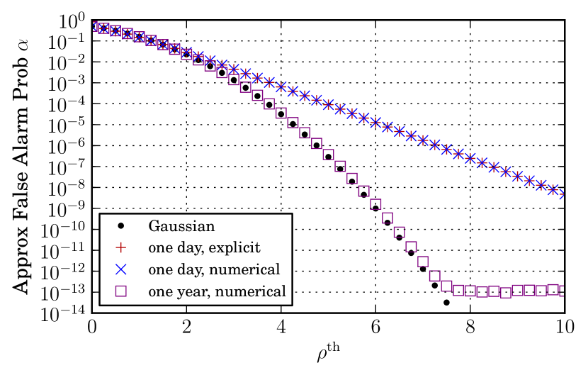
Figure 12: False alarm probabilities for the cross-correlation statistic in the day-long and year-long scenarios considered in Fig. 11, using the explicit formula (168) as well as numerical integration of (169), along with the probabilities we would get if we assumed the statistic to be Gaussian. For a day-long observation (with three detectors, $T_{\text{sft}}=900\text{\,s}$ and $T_{\text{max}}=3600\text{\,s})$, both methods give comparable results, but the Gaussian approximation is invalid for single-template false alarm probabilities below about $10^{-2}$. Note that for large signal values, a single exponential term dominates. For a year-long observation, practical calculation with (168) is impossible due to underflow issues. The numerical integration of (169) becomes unstable for false alarm probabilities below $10^{-12}$, but not before quantifying deviations from the Gaussian approximation even for a year-long observation.

Then

$$\prod_{L\neq K}\left(1-\frac{\omega_{L}}{\omega_{K}}\right)=\left[\prod_{L=1}^{K-1}\left(1-\frac{\omega_{L}}{\omega_{K}}\right)\right]\left[\prod_{L=K+1}^{N}\left(1-\frac{\omega_{L}}{\omega_{K}}\right)\right]\\ =(-1)^{N-K}\left[\prod_{L=1}^{K-1}\left(1-\frac{\omega_{L}}{\omega_{K}}\right)\right]\left[\prod_{L=K+1}^{N}\left(\frac{\omega_{L}}{\omega_{K}}-1\right)\right]$$ (167)

and the false alarm probability is

$$\alpha=\sum_{K=K_{0}}^{N}(-1)^{N-K}e^{-\rho^{\text{th}}/\omega_{K}}\\ \times\left[\prod_{L=1}^{K-1}\left(1-\frac{\omega_{L}}{\omega_{K}}\right)\right]^{-1}\left[\prod_{L=K+1}^{N}\left(\frac{\omega_{L}}{\omega_{K}}-1\right)\right]^{-1}$$ (168)

The last two factors can be very large, and are larger when the eigenvalues are closer together. (Recall that $N$ is the number of SFTs, which is approximately $T_{\text{obs}}/T_{\text{sft}}$, so there are many factors appearing in the product.)

Given the numerical problems with the exact false alarm probability (168) when the number of SFTs is large, it is sometimes necessary to use an alternate approach. We can perform a calculation analogous to that in Goetz and Riles (2011), based on the method of Davies (1973, 1980). This uses the Gil-Pelaez expressionGil-Pelaez (1951) to construct a cumulative distribution directly from the characteristic function (163) according to

$$\alpha=\frac{1}{2}+\frac{1}{\pi}\int_{0}^{\infty}\operatorname{Im}\left(\varphi(t)\,e^{-\mathrm{i}t\rho^{\text{th}}}\right)\frac{dt}{t}$$ (169)

We can then find the false alarm probability by numerical integration of (169). Results of both of these methods are shown in Fig. 12, for the two scenarios considered in Fig. 11. Both methods produce consistent results for a day-long observation, and illustrate deviation of the false alarm probability from the Gaussian value for $\rho^{\text{th}}\gtrsim 2$. For the year-long observation, explicit evaluation of (168) is impossible because of underflow in the cancellations, but numerical integration of (169) works until the false alarm probability goes below $10^{-12}$ or so. False alarm probabilities are considered in detail for a wider range of observing scenarios in Zhang et al. (2015).

References

- Steeghs and Casares (2002) D. Steeghs and J. Casares, “The Mass Donor of Scorpius X-1 Revealed,” Astrophys. J. 568, 273–278 (2002), astro-ph/0107343 .
- Aasi et al. (2015a) J. Aasi et al. (LIGO Scientific Collaboration), “Advanced LIGO,” Class. Quant. Grav. 32, 074001 (2015a), arXiv:1411.4547 .
- Acernese et al. (2015) F. Acernese et al. (Virgo Collaboration), “Advanced Virgo: a second-generation interferometric gravitational wave detector,” Class. Quant. Grav. 32, 024001 (2015), arXiv:1408.3978 .
- Somiya (2012) Kentaro Somiya (for the KAGRA Collaboration), “Detector configuration of KAGRA–The Japanese cryogenic gravitational-wave detector,” Class. Quant. Grav. 29, 124007 (2012), arXiv:1111.7185 .
- Messenger (2011) Chris Messenger, “Semicoherent search strategy for known continuous wave sources in binary systems,” Phys. Rev. D. 84, 083003 (2011), arXiv:1109.0501 .
- Leaci and Prix (2015) Paola Leaci and Reinhard Prix, “Directed searches for continuous gravitational waves from binary systems: parameter-space metrics and optimal Scorpius X-1 sensitivity,” Phys. Rev. D. 91, 102003 (2015), arXiv:1502.00914 .
- Galloway et al. (2014) D. K. Galloway, S. Premachandra, D. Steeghs, T. Marsh, J. Casares, and R. Cornelisse, “Precision Ephemerides for Gravitational-wave Searches. I. Sco X-1,” Astrophys. J. 781, 14 (2014), arXiv:1311.6246 .
- Abbott et al. (2007a) B. Abbott et al. (LIGO Scientific Collaboration), “Searches for periodic gravitational waves from unknown isolated sources and Scorpius X-1: Results from the second LIGO science run,” Phys. Rev. D. 76, 082001 (2007a), arXiv:gr-qc/0605028 .
- Bradshaw et al. (1999) C. F. Bradshaw, E. B. Fomalont, and B. J. Geldzahler, “High-Resolution Parallax Measurements of Scorpius X-1,” Astrophys. J. Lett. 512, L121 (1999).
- Jaranowski et al. (1998) Piotr Jaranowski, Andrzej Krolak, and Bernard F. Schutz, “Data analysis of gravitational-wave signals from spinning neutron stars. I: The signal and its detection,” Phys. Rev. D. 58, 063001 (1998), arXiv:gr-qc/9804014 .
- Andersson et al. (1999) Nils Andersson, Kostas D. Kokkotas, and Nikolaos Stergioulas, “On the relevance of the -mode instability for accreting neutron stars and white dwarfs,” Astrophys. J. 516, 307 (1999), arXiv:astro-ph/9806089 .
- Bildsten (1998) Lars Bildsten, “Gravitational Radiation and Rotation of Accreting Neutron Stars,” Astrophys. J. Lett. 501, L89 (1998), arXiv:astro-ph/9804325 .
- Watts et al. (2008) Anna Watts, Badri Krishnan, Lars Bildsten, and Bernard F. Schutz, “Detecting gravitational wave emission from the known accreting neutron stars,” Mon. Not. R. Astron. Soc. 389, 839–868 (2008), arXiv:0803.4097 .
- Abbott et al. (2007b) B. Abbott et al. (LIGO Scientific Collaboration), “Upper limit map of a background of gravitational waves,” Phys. Rev. D. 76, 082003 (2007b), arXiv:astro-ph/0703234 .
- Ballmer (2006) Stefan W. Ballmer, “A radiometer for stochastic gravitational waves,” Class. Quant. Grav. 23, S179 (2006), gr-qc/0510096 .
- Messenger and Woan (2007) C. Messenger and G. Woan, “A fast search strategy for gravitational waves from low-mass x-ray binaries,” Class. Quant. Grav. 24, S469–S480 (2007), arXiv:gr-qc/0703155 .
- Aasi et al. (2015b) J. Aasi et al. (LIGO Scientific Collaboration and Virgo Collaboration), “Directed search for gravitational waves from Scorpius X-1 with initial LIGO data,” Phys. Rev. D. 91, 062008 (2015b), arXiv:1412.0605 .
- Goetz and Riles (2011) E. Goetz and K. Riles, “An all-sky search algorithm for continuous gravitational waves from spinning neutron stars in binary systems,” Class. Quant. Grav. 28, 215006 (2011), arXiv:1103.1301 .
- Aasi et al. (2014) J. Aasi et al. (LIGO Scientific Collaboration and Virgo Collaboration), “First all-sky search for continuous gravitational waves from unknown sources in binary systems,” Phys. Rev. D. 90, 062010 (2014), arXiv:1405.7904 .
- van der Putten et al. (2010) S. van der Putten, H.J. Bulten, J.F.J. van den Brand, and M. Holtrop, “Searching for gravitational waves from pulsars in binary systems: An all-sky search,” J. Phys. Conf. Ser. 228, 012005 (2010).
- Dhurandhar et al. (2008) Sanjeev Dhurandhar, Badri Krishnan, Himan Mukhopadhyay, and John T. Whelan, “Cross-correlation search for periodic gravitational waves,” Phys. Rev. D. 77, 082001 (2008), arXiv:0712.1578 .
- Chung et al. (2011) Christine Chung, Andrew Melatos, Badri Krishnan, and John T. Whelan, “Designing a cross-correlation search for continuous-wave gravitational radiation from a neutron star in the supernova remnant SNR 1987A,” Mon. Not. R. Astron. Soc. 414, 2650–2663 (2011), arXiv:1102.4654 .
- Prix (2011) Reinhard Prix, “The -statistic and its implementation in ComputeFstatistic_v2,” LIGO Technical Document LIGO-T0900149-v5 (2011).
- Whelan et al. (2010) John T. Whelan, Reinhard Prix, and Deepak Khurana, “Searching for galactic white-dwarf binaries in mock LISA data using an -statistic template bank,” Class. Quant. Grav. 27, 055010 (2010), arXiv:0908.3766 .
- Prix and Whelan (2007) Reinhard Prix and John T. Whelan, “-statistic search for white-dwarf binaries in the first Mock LISA Data Challenge,” Class. Quant. Grav. 24, S565 (2007), arXiv:0707.0128 .
- Abbott et al. (2008) B. Abbott et al. (LIGO Scientific Collaboration), “All-sky search for periodic gravitational waves in LIGO S4 data,” Phys. Rev. D. 77, 022001 (2008), arXiv:0708.3818 .
- Sundaresan and Whelan (2012) Santosh Sundaresan and John T. Whelan, “Windowing and leakage in the cross-correlation search for periodic gravitational waves,” LIGO Technical Document LIGO-T1200431-v1 (2012).
- Zhang et al. (2015) Yuanhao Zhang, John T. Whelan, and Badri Krishnan, “Results of a Model-Based Cross-Correlation Search for Signals from Scorpius X-1 in Mock Gravitational-Wave Data,” LIGO DCC P1400216 (2015).
- Wette (2012) Karl Wette, “Estimating the sensitivity of wide-parameter-space searches for gravitational-wave pulsars,” Phys. Rev. D. 85, 042003 (2012), arXiv:1111.5650 .
- Abadie et al. (2011) J.. Abadie et al. (LIGO Scientific Collaboration and Virgo Collaboration), “Directional Limits on Persistent Gravitational Waves Using LIGO S5 Science Data,” Phys. Rev. Lett. 107, 271102 (2011), arXiv:1109.1809 .
- Abbott et al. (2004) B. Abbott et al. (LIGO Scientific Collaboration), “Analysis of first LIGO science data for stochastic gravitational waves,” Phys. Rev. D. 69, 122004 (2004), arXiv:gr-qc/0312088 .
- Messenger et al. (2015) C. Messenger et al., “Gravitational waves from Sco X-1: A comparison of search methods and prospects for detection with advanced detectors,” (2015), arXiv:1504.05889 .
- Brady et al. (1998) Patrick R. Brady, Teviet Creighton, Curt Cutler, and Bernard F. Schutz, “Searching for periodic sources with LIGO,” Phys. Rev. D. 57, 2101 (1998), arXiv:gr-qc/9702050 .
- Prix (2007) Reinhard Prix, “Search for continuous gravitational waves: Metric of the multi-detector -statistic,” Phys. Rev. D. 75, 023004 (2007), arXiv:gr-qc/0606088 .
- Gallager (2014) Robert G. Gallager, Stochastic Processes: Theory for Applications (Cambridge University Press, Cambridge, England, 2014).
- Davies (1973) R. B. Davies, “Numerical inversion of a characteristic function,” Biometrika 60, 415 (1973).
- Davies (1980) Robert B. Davies, “Algorithm AS 155: The Distribution of a Linear Combination of Random Variables,” J. Roy. Stat. Soc., Series C 29, 323 (1980).
- Gil-Pelaez (1951) J. Gil-Pelaez, “Note on the inversion theorem,” Biometrika 38, 481 (1951).