Gravitational waves from Sco X-1: A comparison of search methods
and prospects for detection with advanced detectors

Abstract

The low-mass X-ray binary Scorpius X-1 (Sco X-1) is potentially the most luminous source of continuous gravitational-wave radiation for interferometers such as LIGO and Virgo. For low-mass X-ray binaries this radiation would be sustained by active accretion of matter from its binary companion. With the Advanced Detector Era fast approaching, work is underway to develop an array of robust tools for maximizing the science and detection potential of Sco X-1. We describe the plans and progress of a project designed to compare the numerous independent search algorithms currently available. We employ a mock-data challenge in which the search pipelines are tested for their relative proficiencies in parameter estimation, computational efficiency, robustness, and most importantly, search sensitivity. The mock-data challenge data contains an ensemble of 50 Scorpius X-1 (Sco X-1) type signals, simulated within a frequency band of 50–1500 Hz. Simulated detector noise was generated assuming the expected best strain sensitivity of Advanced LIGOAasi et al. (2015) and Advanced VIRGOAcernese et al. (2015a) ($4\times 10^{-24}$ Hz^-1/2). A distribution of signal amplitudes was then chosen so as to allow a useful comparison of search methodologies. A factor of 2 in strain separates the quietest detected signal, at $6.8\times 10^{-26}$ strain, from the torque-balance limit at a spin frequency of 300 Hz, although this limit could range from $1.2\times 10^{-25}$ (25 Hz) to $2.2\times 10^{-26}$ (750 Hz) depending on the unknown frequency of Sco X-1. With future improvements to the search algorithms and using advanced detector data, our expectations for probing below the theoretical torque-balance strain limit are optimistic.

I Introduction

Low-mass X-ray binaries (LMXBs) are one of the most promising sources of continuous gravitational-wave (GW) emission for ground-based GW detectors. This precedence is motivated by the availability of an accretion-driven power source in these systems potentially capable of generating and supporting non-axisymmetric distortions in the Neutron Star (NS) component Papaloizou and Pringle (1978); Wagoner (1984); Bildsten (1998); Ushomirsky et al. (2000); Cutler (2002). low-mass X-ray binaries, and specifically sources such as Sco X-1 and Cygnus X-2 Premachandra (2015) are prime targets for GW searches. Since the second LIGO Science Run, numerous searches have been performed for Sco X-1 using varied data analysis strategies Abbott et al. (2007a, b, 2011); Aasi et al. (2014a, b), resulting in non-detections, but with increasing sensitivity. Sco X-1 is identified as the most likely, strongest GW emitter of the currently-known LMXBs due to its relative proximity to Earth and its high accretion rate. The accretion rate is used to infer the possible amplitude of GWs emitted according to the torque-balance model proposed in Wagoner (1984). With the forthcoming and unprecedented sensitivity from the advanced GW detectors The LIGO Scientific Collaboration et al. (2015); LIGO Scientific Collaboration et al. (2013); Harry (2010); Acernese et al. (2015b), our goal is detecting this source or performing more astrophysically constraining non-detections. In the latter case, the analyses would eventually be probing signal amplitudes that are below the current torque-balance limit and hence constraining LMXB accretion models.

The parameters governing the expected phase evolution of a continuous GW signal from Sco X-1 are only partially constrained. The Sco X-1 system is believed to contain a NS, but unlike a subset of other LMXBs Roy et al. (2015); Deller et al. (2014); Tendulkar et al. (2014); Bogdanov et al. (2014), the NS exhibits neither persistent nor intermittent pulsations in any electromagnetic band, and hence the spin frequency of the NS is unknown. This non-pulsating property has consequences for the estimation of the orbital parameters of the system, which are currently constrained through optical observations of the lower-mass companion object Steeghs and Casares (2002); Galloway et al. (2014). Additionally, there are relatively large uncertainties in the intrinsic spin evolution of the NS since it is constantly under the influence of a high rate of accretion from its companion. Consequently, the volume of the search parameter space is vast and computationally prohibitive for the most sensitive type of approach—the fully-coherent, matched-filter search over a bank of filters.

Other approaches to the detection problem attempt to maximize detection probability with a limited computational cost and are the best strategy for this problem. Numerous such methods have been developed within the GW community over the past decade. Most have been designed with other types of continuous GW sources as targets, but many are also suitable, with appropriate tuning, to the Sco X-1 problem. For this reason, we performed the study presented in this article. The principal objective is to compare and contrast the detection capabilities and parameter estimation properties of the numerous search methods presently available for Sco X-1. A mock-data challenge (MDC) is the best approach to identify commonalities and differences between analysis methods. The MDC includes many Sco X-1-type signals (with parameter values unknown to the partcipants) that are simulated in noise and analyzed by the various search pipelines in parallel. Since this is the first MDC of its kind for Sco X-1, the focus here is on a comparison between pipelines rather than including astrophysically realistic signal amplitudes. We anticipate a future MDC that employs more realistic signal parameters in order to more fully approximate a true search for continuous GWs from Sco X-1.

This article is organized as follows. Section II is a description of the Sco X-1 system, with focus on the possible emission mechanisms and on the state of knowledge of those parameters that influence the form of a continuous GW signal. In Section III brief descriptions and relevant references to the search pipelines that have participated in the MDC are given. Section IV contains a qualitative comparison of the search pipelines and the design and implementation of the MDC itself is presented in Section V. The results from each search pipeline are reported in Section VI and the manuscript concludes with Section VII containing a discussion of our findings and plans for future pipelines, pipeline improvements and a more realistic future MDCs.

II Scorpius X-1

Sco X-1 is a binary system with an orbital period of approximately 18.9 h, likely consisting of a $\sim$$1.4M_{\odot}$ NS that accretes mass from a $0.42M_{\odot}$ companion Steeghs and Casares (2002). With a long-term average X-ray flux of $3.9\times 10^{-10}\,\mathrm{W}\,{\mathrm{m}}^{-2}$ Watts et al. (2008), it is the brightest continuous extrasolar X-ray source on the sky, indicating a comparatively high accretion rate.

It has been proposed Bildsten (1998) that in a stable, X-ray luminous NS binary system like Sco X-1, the angular momentum transferred from the low-mass companion to the NS and the energy loss due to gravitational radiation are in equilibrium. Since the former can be deduced from the X-ray flux, torque-balance leads to a GW strain amplitude as a function of the spin frequency $\nu_{\text{s}}$ for Sco X-1 of Bildsten (1998); Galloway et al. (2014)

$$h_{0}\approx 3.5\times 10^{-26}\sqrt{\frac{300\,\mathrm{Hz}}{\nu_{\text{s}}}}\,.$$ (1)

It is possible that the system could temporarily be in a state where accretion torque exceeds the GW torque while maintaining the long term torque balance on average. This could result in a temporary increase in the strength of GW emission Haskell et al. (2015). Considering the long term average, if the spin frequency is between $25\,\mathrm{Hz}$ and $750\,\mathrm{Hz}$, the torque-balance strain is between $2.2\times 10^{-26}$ and $1.2\times 10^{-25}$.

There is significant astrophysical uncertainty in the torque-balance limit. Its derivation assumes accretion of mass at the radius of the neutron star, but the effective accretion radius for angular momentum transfer may be closer to the Alfvén radius, leading to a higher strain limit. On the other hand, its derivation also assumes negligible angular momentum loss from the star other than from GW emission and hence may be too high.

In a GW interferometer, this strain would be recorded (circular-orbit approximation) as $h(t)$:

$$\begin{split}h(t)=&\ h_{0}F_{+}(t,\alpha,\delta,\psi)\frac{1+\cos^{2}(\iota)}{2}\cos[\Phi(t)]\\ &+h_{0}F_{\times}(t,\alpha,\delta,\psi)\cos(\iota)\sin[\Phi(t)]\,,\end{split}$$ (2a)

$$\Phi(t)= \ \Phi_{0}+2\pi f_{0}(t_{\text{bin}}-t_{\text{ref}})+\delta\Phi_{\textup{spin-wander}}$$ (2b)

$$t_{\text{bin}}= \ t-d(t)-(a\sin i)\sin[2\pi(t-T_{\text{asc}})/P]\,.$$ (2c)

where $h_{0}$ is strain in the solar system barycenter, $F_{+}$ and $F_{\times}$ are detector antenna patterns for plus- and cross-polarizations, $t$ is time the signal is received at the detector, $\alpha$ and $\delta$ are respectively right ascension and declination, $\psi$ is polarization angle, $\iota$ is the inclination angle of the neutron star with respect to the line of sight, $f_{0}$ is the intrinsic signal frequency, $\Phi_{0}$ is the GW phase at reference time $t_{\textup{ref}}$, $d(t)$ and $a\sin i$ are the projections respectively of the detector’s separation relative to the solar system barycentre and the orbital semimajor axis onto the line of sight (where $i$ is the inclination angle of the LMXB orbit with respect to the line of sight), both measured in units of time, $P$ is the orbital period, $T_{\text{asc}}$ is the time of the orbital ascending node, and $\delta\Phi_{\textup{spin-wander}}$ is a unknown quantity accounting for spin-wandering induced by the short-term variation in accreted mass from the companion star.

II.1 The parameter space

Sco X-1 has been studied widely due to its prominence in the LMXB population. It is relatively nearby, at a distance (estimated from radio parallax measurements) of $2.8\pm 0.3$ kpc Bradshaw et al. (1999). Thanks in part to the relatively low extinction, the optical counterpart, V818 Sco, is also unusually bright for a LMXB ($V\approx 12.5$; Liu et al. (2007)).

The parameters that completely describe the binary system (for the purposes of the gravitational wave searches) are the orbital period $P$; reference phase $T_{\text{asc}}$ (the ascending node, i.e. the time at which the compact object crosses the plane tangent to the sky, moving away from the observer); and the projected semi-major axis $a\sin i$, where $i$ is the angle of the orbit’s axis relative to our line of sight (Table 1). In addition, it may be necessary to consider the limits on the system eccentricity $e$, (e.g. Galloway et al. (2014); Leaci and Prix (2015)), may require more than one template to span the parameter uncertainty interval.

The most precise orbital parameter measurements have been made from analysis of the Bowen blend emission lines around 4640 Å in the optical spectrum, arising from N iii and C iii Steeghs and Casares (2002). These emission lines are known to arise from the heated side of the companion facing the neutron star, and so by repeat measurements of their radial velocity, the orbital period and phase can be measured. The most recent effort combined two epochs of radial velocity measurements over a 12-yr baseline, to obtain an orbital period of $P=0.7873114\pm 0.0000005$ d and a time of inferior conjunction of the companion of $T_{0}=2454635.3683\pm 0.0012$ HJD Galloway et al. (2014).

Because these measurements track the companion (rather than the neutron star that is the source of the GW emission) the reference epoch must be shifted by for the purposes of GW searches. To convert from $T_{0}$ (when the companion is closest to the observer) to $T_{\text{asc}}$ (when the compact object crosses the plane of the sky moving away from the observer, one must take $T_{\text{asc}}=T_{0}-P/4=2454635.1715\pm 0.0012$ HJD. Furthermore, because the reference phase is defined at a particular epoch (depending upon the span of data used in the radial velocity fits), the effective uncertainty in $T_{\text{asc}}$ increases towards earlier and later times, and this increase must be taken into account for future GW searches. This effect was quantified by Galloway et al. (2014), including the effects of additional observational efforts.

The projected semi-major axis of the neutron star orbit $a\sin i$ is the most challenging to measure. It can be obtained in principle from the velocity amplitude of the Bowen emission region on the face of the companion, but this requires a correction first to the companion’s center of mass, and then to the neutron star, which requires constraints on the companion radius as well as the mass ratio of the binary components. This parameter is estimated instead from the symmetric component of the Doppler tomogram of the broad emission lines in the system as $1.44\pm 0.18$ lt-s (derived from a velocity amplitude of $K_{1}=40\pm 5\ {\rm km\,s^{-1}}$) Steeghs and Casares (2002). However, the Doppler tomogram derived from the subsequent epoch of optical spectroscopy analyzed by Galloway et al. (2014), exhibited significantly different morphology, such that it was not possible to (for example) combine the two datasets to improve the precision of the $a\sin i$ estimate.

While further incremental improvements on $P$ and $T_{\text{asc}}$ can be achieved relatively easily with additional optical spectroscopic measurements, improving the estimate of $a\sin i$ will likely require a deeper understanding of how the emission line morphology in the system evolves in response to secular variations.

In contrast to the binary system parameters, the spin frequency of the neutron star is unknown. No persistent or intermittent X-ray pulsations have been detected from Sco X-1. While the accreting source is thought to be a neutron star, no thermonuclear (“type-I”) bursts have ever been detected from the source, and hence no “burst oscillations” have been observed. Non-detections for X-ray pulsations have been reported for searches up to frequencies of 256 Hz, using data obtained with the European X-ray Observatory Satellite (EXOSAT; Middleditch and Priedhorsky (1986)), and up to 512 Hz using observations by Ginga Wood et al. (1991); Hertz et al. (1992); Vaughan et al. (1994). A much larger set (approximately 1.3 Ms) of high-time resolution (down to $1\ \mu s$) data is available from the Rossi X-ray Timing Explorer (RXTE; Jahoda et al. (1996)) mission (1996–2012). While unsuccessful searches of these data have almost certainly taken place (due to both the prominence of Sco X-1 among the LMXB population, and the high priority for pulsation searches for this mission) no limits have been reported. Analysis of these data are hampered by the high count-rate of the source, which necessitates non-standard data modes, as well as introducing substantial effects from instrumental “dead-time”.

The likely frequency range for the spin period has been estimated based on the separation of a pair of high-frequency quasi-periodic oscillations (QPOs), measured in the range 240–310 Hz van der Klis et al. (1996, 1997); Méndez and van der Klis (2000). In sources that exhibit pulsations or burst oscillations in addition to pairs of kHz QPOs, the QPO frequency separation is roughly equal to the spin frequency (or half that value).

Table 1: Scorpius X-1: system parameters

Sco X-1 parameter	Value	Uncertainty	Ref
Period	68023.70 sec	0.04 sec	Galloway et al. (2014)
Orbital semi-major axis	1.44 sec	0.18 sec	Abbott et al. (2007b); Steeghs and Casares (2002)
Time of ascension	897753994	100 sec	Galloway et al. (2014)
Orbital eccentricity	$<0.068$	$3\sigma$	Galloway et al. (2014); Leaci and Prix (2015)
Right Ascension	$16^{\mathrm{h}}19^{\mathrm{m}}55^{\mathrm{s}}.067$	$0\mbox{$.\!\!^{\prime\prime}$}06$	Skrutskie et al. (2006)
Declination	$-15^{\circ}38\mbox{${}^{\prime}$}25\mbox{$.\!\!^{\prime\prime}$}02$	$0\mbox{$.\!\!^{\prime\prime}$}06$	Skrutskie et al. (2006)
System inclination	$44^{\circ}$	$6^{\circ}$	Fomalont et al. (2001)
Companion mass	0.42 M${}_{\textup{Sol}}$		Steeghs and Casares (2002)
X-ray flux	$3.9\times 10^{-10}\mathrm{Wm}^{-2}$		Watts et al. (2008)

Note that the time of ascension ($T_{\rm asc}$) refers to the neutron star, and is calculated as $T_{0}-P/4$, where $T_{0}$ is the epoch of inferior conjunction of the companion from Galloway et al. (2014). The radial velocity data from this paper were also the source of the eccentricity limit, which was calculated by the authors.

Accreting neutron stars exhibit “spin wandering” (gradual changes in spin frequency; e.g. Bildsten et al. (1997); Baykal and Oegelman (1993)), attributed primarily to variations in the accretion rate. The accretion rate in turn varies on timescales of minutes to decades, with most notably, transient sources exhibiting outbursts during which the accretion rate increases by several orders of magnitude compared to the quiescent level King (2006). As a result, GW searches for LMXB systems are necessarily limited to a coherence time equal to the maximum timescale over which the spin evolution can be well modelled.

Although observations of the radio jets from Sco X-1 can be used under model-dependent assumptions to constrain the orientation of the neutron star spin axis Fomalont et al. (2001), here we assume no a priori knowledge of the axis direction.

III Current and future methods

In this section we give an overview of the current search algorithms (or pipelines) available for searches targeting Sco X-1. For additional technical details we either refer the reader to the corresponding methodological papers for each algorithm, where possible, or to a corresponding Appendix. In the following sections, we describe six algorithms: four which were used in our original comparison study, one for which the analysis infrastructure was completed after the initial deadline and run in self-blinded mode on the same data set in the subsequent months as described in Table 5, and one that has been proposed for future analyses.

III.1 Polynomial Search

The Polynomial Search van der Putten et al. (2010) is a generic all-sky method for finding GWs from continuously emitting sources, such as NSs in binary systems, in GW interferometric data. It is based on the assumption that the phase of an expected signal due to these sources in a ground-based GW detector can be approximated by a third-order polynomial in time during short stretches of time. If the binary orbit is the dominant source of Doppler modulation in the signal, this holds for periods up to one quarter of the binary period.

For each input short Fourier transform (SFT), the algorithm generates a set of templates of signals with a phase $\Phi_{t}(t)$ that evolves as a polynomial in time.

$$\Phi_{t}(t)=2\pi\left[f_{0}t+\frac{c_{1}}{2}t^{2}+\frac{c_{2}}{6}t^{3}\right]$$ (3)

The range for the polynomial coefficients $f_{0}$, $c_{1}$ and $c_{2}$ are chosen prior to analysis based on the properties of expected signals. The initial phase is matched implicitly by allowing for an offset in time between data and template.

The correlation of each template with the data segment is calculated as a function of offset time by multiplication in the frequency domain. The offset time that yields the largest correlation value is then recorded.

The probability that one or more templates yield a correlation exceeding a thresold value $C_{\text{t}}$ due to noise is

$$p_{\mathrm{SFT}}(C_{\text{t}})=1-{\left[\frac{1}{2}+\frac{1}{2}\operatorname{erf}\left(\frac{C_{t}}{\sqrt{2}\sigma}\right)\right]}^{N_{e}}$$ (4)

where $\sigma$ is the square root of the average power contained in an SFT frequency bin and $N_{e}$ is the effective number of templates. While the number of templates $N$ is known exactly, there is some degree of overlap between successive templates and $N_{e}$ corrects for this overlap. It can be determined by fitting the measured false alarm rate versus correlation threshold $C_{\text{t}}$ on the analysis results of a data set that contains only noise.

When analyzing $N$ SFTs with pure noise, the probability $p(n)$ that $n$ or more SFTs have one or more templates with a correlation exceeding the threshold is governed by a cumulative binomial distribution with a per-trial probability given by equation (4). This is the single-trial test statistic for detection. In order to test against a chosen false alarm probability threshold, the threshold is divided by the number of frequency bins to correct for the multiple comparisons problem Bonferroni (1935, 1936).

The Polynomial Search is an all-sky search and it does not benefit from detailed knowledge of the source that only influences the phase or the amplitude of the signal, however orbital parameters put a constraint on the time derivatives of the frequency in the data and the orbital period of Sco X-1 can be exploited by using longer SFTs than would be feasible for an all-sky search, increasing the coherence time and therefore also the sensitivity.

III.2 Radiometer

The Radiometer analysis Ballmer (2006); Abbott et al. (2007a, 2011) cross-correlates data from pairs of detectors to detect GW point sources with minimal assumptions about the signal, and uses an estimator given by

$$\hat{Y}=\int_{-\infty}^{\infty}df\int_{-\infty}^{\infty}df^{\prime}\delta_{T}(f-f^{\prime}){\tilde{s}}^{*}_{1}(f){\tilde{s}}_{2}(f^{\prime}){\tilde{Q}}(f^{\prime})$$ (5)

with variance

$$\sigma^{2}_{Y}\approx\frac{T}{2}\int_{0}^{\infty}dfP_{1}(f)P_{2}(f)|{{\tilde{Q}}(f)}|^{2}\,.$$ (6)

Here, $\delta_{T}(f-f^{\prime})$ is the finite-time approximation to the Dirac delta function, ${\tilde{s}}_{1}$ and ${\tilde{s}}_{2}$ are Fourier transforms of time-series strain data for each detector in the pair, $T$ is the detector pair live-time, and $P_{1}$ and $P_{2}$ are one-sided strain power spectral densities for each detector. The cross-correlation is performed with an optimal filter function, ${\tilde{Q}}(f)$, which weights time and frequency bins based on their sensitivity. The filter depends upon the modeled strain power spectrum and is normalized by the strain noise power spectra of the detector pairs. Also included in the filter is a phase factor which takes into account the time delay between the two detector sites. The detection statistic, the Radiometer signal-to-noise ratio (SNR) known as the ‘$Y$-statistic’, is calculated using a weighted average of data from many segments and multiple detector pairs:

$${\hat{Y}_{\rm tot}=\frac{\sum_{l}\hat{Y}_{l}\sigma_{l}^{-2}}{\sum_{l}\sigma_{l}^{-2}}}$$ (7)

with total variance

$${\sigma_{\rm tot}^{-2}=\sum_{l}\sigma_{l}^{-2}\,}$$ (8)

where $l$ sums over time segments and/or detector pairs for the variables defined in (5) and (6). It is expected to be normally distributed from the central limit theorem, and indeed this is born out empirically Abbott et al. (2007a, 2011). The Radiometer $Y$-statistic is the optimal maximum likelihood estimator for a cross-correlation search Ballmer (2006).

In practice, the Radiometer method has also been shown to yield robust results in the presence of realistic (non-Gaussian) noise Abbott et al. (2007a, 2011). The Radiometer search does not use a matched filter; so there are no assumptions about time evolution, except that the signal frequency remains within the 0.25 Hz frequency bin searched (0.25 Hz frequency bins were chosen based on the convention of other applications of the Radiometer algorithm and are not optimized for the Sco X-1 analysis). By not employing a matched filter, the Radiometer loses the sensitivity possible from using prior knowledge about the waveform. For the same reason, however, it is sensitive to arbitrary signal models (within the observing band), and is therefore robust.

III.3 Sideband search

The “Sideband” search Messenger and Woan (2007); Sammut et al. (2014) is based on an approach used in the detection of radio pulsars and low-mass X-ray binaries emitting Electromagnetic (EM) radiation Ransom et al. (2003). It uses the fact that the power in a continuously emitted signal from a source in a binary system, when observed over many orbits, becomes distributed among a finite number of frequency-modulated sidebands. These sidebands have the property that there is always a fixed number of sidebands for a given source. This number is dependent only upon the intrinsic emission frequency and the orbital radius. The frequency separation of the sidebands is the inverse of the orbital period, and the phasing relation between sidebands is a function of the orbital phase. The power spectrum of a timeseries containing such a signal will therefore be independent of the orbital phase. For a source of known orbital period and reasonably well constrained orbital radius (e.g. Sco X-1) the characteristic “comb”-like structure is well-defined and the data analysis task becomes one of locating this frequency domain structure.

In this case it is computationally efficient to construct a template in the frequency domain that closely matches the main features of this structure i.e. the width of the comb and the separation of the teeth. This template is then convolved with the $\mathcal{F}$-statistic Jaranowski et al. (1998) yielding a frequency series that contains the summed power from all sidebands as a function of central intrinsic emission frequency. The $\mathcal{F}$-statistic is used instead of the power spectrum due to the quadrupole emission of GWs coupled with the time-varying detector response. This is computed as a function of frequency and for the known fixed sky position allowing the effects of the motion of the detector relative to the source to be removed from the data. The convolution of the template with the $\mathcal{F}$-statistic, known as the $\mathcal{C}$-statistic, is given by

$$\mathcal{C}(f) =\sum\limits_{j}2\mathcal{F}(f_{j})\mathcal{T}(f_{j}-f)$$

$$=\left(2\mathcal{F}\ast\mathcal{T}\right)(f)$$ (9)

where $2\mathcal{F}$ is the $\mathcal{F}$-statistic and $\mathcal{T}$ is the comb template. Although this statistic is the incoherent sum of power from many sidebands, and is hence less sensitive than a fully coherent search, it does have the following qualities. It is very efficient to compute since its only search dimension is frequency and therefore only requires the computation of a fixed set of Fourier transforms. Also, unlike other semi-coherent search algorithms, its sensitivity does not scale with the fourth-root of the observation time. Its incoherent summation occurs in the frequency domain and its sensitivity is therefore proportional to the fourth-root of the number of sidebands. It maintains a square-root sensitivity relation to the observation time.

III.4 TwoSpect

The TwoSpect method Goetz and Riles (2011) relies on computing a sequence of power spectra whose coherence length is short enough so that a putative signal would remain in a single frequency bin during a single spectrum. Thus the coherence length is typically no longer than 1800 seconds; for the Scorpius X-1 search, it is either 360 or 840 seconds, depending on search frequency. For comparison, the sampling frequency of raw data is typically 16384 Hz, and observation runs are millions of seconds long. After the sequence of power spectra are corrected for the Doppler shift caused by Earth’s motion, a periodogram is created. For each frequency bin in the periodogram, we compute a second Fourier Transform, for which the integrated variable is the time of each power spectrum. When a continuous GW signal is present in the data, the second power spectra will contain excess power at frequencies corresponding to the GW signal frequency in the first spectra computed, and also the inverse of the binary orbital period in the second power spectrum. The name TwoSpect is given to this algorithm because two successive Fourier transforms are computed.

Gravitational wave detector data are analyzed by creating templates that mimic the putative signal pattern. A detection statistic, $R$, is computed by a weighted sum of $M$ pixel powers in the second Fourier transform $Z_{i}$, subtracting estimated noise $\lambda_{i}$, where the weights $w_{i}$ are determined by the template values for $M$ pixels:

$$R=\frac{\Sigma_{i=0}^{M-1}w_{i}\left[Z_{i}-\lambda_{i}\right]}{\Sigma_{i=0}^{M-1}\left[w_{i}\right]^{2}}\,.$$ (10)

To create a template for a circular orbit binary system, the putative GW signal frequency, binary orbital period, and amplitude of the frequency modulation are given. Orbital phase is an unimportant parameter due to the nature of the analysis: computing successive power spectra from the SFTs and then, importantly, the second second Fourier transforms remove dependence on orbital phase.

Although the original design of TwoSpect was an all-sky search method Goetz and Riles (2011); Aasi et al. (2014a), it can also be used as a directed search algorithm. By design, it is robust against phase jumps of the signal between successive power spectra, and TwoSpect is unaffected by spin wandering of sources because of the semi-coherent nature of the method and because of the short coherence time of the first Fourier transform. The choice of the coherence length of the first series of power spectra is given by the putative amplitude and period of the frequency modulation caused by the motion of the source. With these features, the TwoSpect method is a computationally efficient and robust algorithm capable of analyzing long stretches of gravitational wave data and detecting continuous GW signals from NSs in binary systems.

Running TwoSpect as a directed search algorithm involves calculating the $R$-detection statistic in the parameter space that might contain the GW signal (the incoherent harmonic sum stage of TwoSpect, used for the all-sky search, was bypassed entirely). The orbital period of Sco X-1 is sufficiently well-known to restrict the search to the two dimensions of putative signal frequency and frequency modulation. The grid spacing, inversely proportional to spectrum coherence time, was chosen to allow a mismatch of no more than $0.2$ in the detection statistic. Mismatch, in this context, means the relative loss in the the detection statistic, $R$, where the spacing was informed by studies in the TwoSpect methods paper Goetz and Riles (2011).

III.5 Cross-Correlation

The cross-correlation method Dhurandhar et al. (2008); Chung et al. (2011); Whelan et al. (2015), henceforth referred to as the CrossCorr method, is a modification of the directed stochastic-background search described in Section III.2. By using the signal model, it is able to coherently combine not just data taken by different detectors at the same time, but also data taken at different times, by the same or different detectors. Since this signal model depends on parameters such as frequency and binary orbital parameters, the search must be repeated over a grid of points in parameter space. In order to control computational costs associated with parameter space resolution, the method limits the time offset between pairs of data segments included in the construction of the statistic, allowing a tradeoff between computation time and sensitivity.

The data from each detector are divided into segments of length $T_{\text{sft}}$, which are then Fourier transformed. The index $K$ is used to label an SFT (so that it encodes both the time of the data segment and the detector from which it’s taken). We construct a statistic

$$\rho=\sum_{KL\in\mathcal{P}}(W_{KL}z_{K}^{*}z_{L}+W_{KL}^{*}z_{K}z_{L}^{*})$$ (11)

using the product of data from SFTs $K$ and $L$, where $KL$ (or $LK$) is in a list of allowed pairs $\mathcal{P}$, defined by $K\neq L$ and $\left\lvert T_{K}-T_{L}\right\rvert\leq T_{\text{max}}$, i.e., the timestamps of the two different data segments should differ by no more than some specified lag time. The weighting factor $W_{KL}$ is determined by the expected signal and noise contributions to the cross-correlation, and the frequency bin or bins used to create the normalized data value $z_{K}$ out of SFT $K$ is determined by the Doppler-shifted signal frequency associated with the modelled signal parameters. The linear combination of cross-correlation terms is normalized so that $\operatorname{Var}(\rho)=1$, and weighted to maximize $E[\rho]$ in the presence of the modelled signal. With this choice of weighting, the expected statistic value for a given $h_{0}$ scales like

$$E[\rho]\sim(h_{0}^{\text{eff}})^{2}\sqrt{T_{\text{obs}}T_{\text{max}}\left\langle\frac{(\Gamma^{\text{ave}}_{KL})^{2}}{S_{K}S_{L}}\right\rangle_{KL\in\mathcal{P}}}$$ (12)

where $h_{0}^{\text{eff}}$ is the combination of $h_{0}$ and $\cos\iota$ defined in (19), $S_{K}$ is constructed from the noise power spectrum and $\Gamma^{\text{ave}}_{KL}$ from the antenna patterns for detectors $K$ and $L$ at the appropriate times. The search can be made more sensitive by increasing $T_{\text{max}}$, but at the cost of additional computing cost, as detailed in Section IV.3.

III.6 Future method: Stacked $\mathcal{F}$-statistic

We now describe a method which has not yet been implemented or run on the MDC data, but holds promise for the future. The distributed computing project Einstein@Home website ; Aasi et al. (2013) was originally designed to undertake the highly computational task of searching for unknown isolated continuous GW sources. This involves a wide frequency band, all-sky search using computing power volunteered by participants across the globe. In recent years this power has been shared between algorithmically similar searches of radio data from the Arecibo and Parkes radio telescopes Knispel et al. (2011, 2013); Allen et al. (2013) and gamma-ray data from the the Fermi telescope.Pletsch et al. (2013)

The GW search uses an algorithm that coherently computes a maximum likelihood statistic over a finite length of data on a bank of signal templates. This statistic is known as the $\mathcal{F}$-statistic Jaranowski et al. (1998); Prix (2007) which is then incoherently summed (or stacked) over segments in such a way as to track a potential signal between segments Brady and Creighton (2000); Wette (2012); Prix and Shaltev (2012). The computational cost of this search is primarily controlled via the ratio of the coherence length to total data length. This is tuned to return approximate optimal sensitivity for the fixed and large computational power available from the Einstein@Home project.

Currently under development is a fixed-sky-location, binary-source version of this search algorithm. In this case the binary parameter space replaces that of the sky. A recent feasibility study Leaci and Prix (2015) investigated the potential sensitivity to Sco X-1.

IV Comparison of methods

In this section, we discuss the general properties of the five algorithms taking part in the MDC in terms of i) their dependence on the parameter space, ii) their intrinsic parameter estimation ability, and iii) their computational cost.

IV.1 Parameter space dependence

Each algorithm’s performance in relation to computational cost, search sensitivity and how the search is setup, depends on the Sco X-1 parameter space. Both the Polynomial and the Radiometer searches have the least parameter space dependence while the Sideband search has the most. The TwoSpect and CrossCorr searches fall between these extremes.

Since the Polynomial search does not explicitly model any of the source orbital parameters, changes in the parameter space boundaries only have indirect effects. For effective detection, the template parameters need to approximate the time derivatives of the phase of the signal as received by the detector. The contributions due to the binary orbit to these derivatives are proportional to the $a\sin i$ and inversely proportional to $P^{2}$ and $P^{3}$ for the first and second derivative of frequency with respect to time, respectively. Additionally, both derivatives scale with $f_{0}$. Therefore, the boundaries of the $c_{1}$ and $c_{2}$ template parameters need to be set to reflect the range of values of $P$ and $a\sin i$ compatible with measurements.

As long as the data contains at least one full binary period, the time of ascension should not affect the Polynomial search’s sensitivity.

Like the Polynomial search, the Radiometer search does not explicitly model and is largely insensitive to the orbital parameters. It operates under the assumption that the instantaneous received frequency of the signal resides within a single 0.25 Hz bin for the duration of the observation. The total expected variation of the instantaneous frequency is proportional to the product of the intrinsic frequency, the orbital semi-major axis and the orbital angular frequency. However, the intrinsic frequency is uncertain over a large range and hence at values in excess of $\sim$1 kHz it is increasingly likely that the assumption that the signal is restricted to a single bin is invalidated. The corresponding effects on sensitivity (and the related conversion factors for $h_{0}$ estimates and their uncertainties) are discussed in Appendix B. The current version of the search also assumes that the signal is circularly polarized. This assumption does not make the search insensitive to other polarizations, however it does affect resulting estimates of the signal amplitude $h_{0}$. To account for the assumption on polarization an average conversion factor can be applied to $h_{0}$ estimates and the associated uncertainties (see Appendix B). If information on the polarization were available, this would change the conversion factor and reduce the associated uncertainty.

The Sideband search in its current form is heavily restricted to the analysis of signals with well-known orbital periods and sky positions. The orbital period defines the spacing between the frequency-domain template “teeth” and knowledge of the sky location allows the coherent demodulation of the detector motion with respect to the source binary barycenter. The search is as sensitive to the source sky location as a fully coherent search. For a 1-year-long observation of a source with frequency $1$ kHz, the sky position must be known to a precision of $\sim$0.1 arcsec. In reality, spin wandering limits observation times for Sideband searches of Sco X-1 to $\sim$10 days Aasi et al. (2014b), which significantly relaxes the restriction on the sky position. The fractional orbital period uncertainty must be $<(4\pi fa\sin iT/P)^{-1}$ which is $\leq 4\times 10^{-6}$ for a 10 day observation of Sco X-1. The orbital semi-major axis determines the width of the frequency domain template which needs to be known to $\sim$10% precision. Post-processing techniques allow using any level of prior knowledge of the NS orientation parameters to be folded into our parameter estimation. The search is completely insensitive to knowledge of the orbital phase of the source, but is extremely sensitive to spin-wandering since the intrinsic frequency resolution is ${\approx}1/T$ where $T$ is the total observation time.

The TwoSpect search is sensitive to projected semi-major axis and orbital period, but is insensitive to initial orbital phase. The two Fourier transforms in TwoSpect preserve only power information at present, ignoring orbital phase. Orbital period can be explored, with a template spacing Goetz and Riles (2011) of $\Delta P\simeq P_{0}^{2}/(\alpha_{\textup{TS}}T_{obs})$ for an allowed detection statistic mismatch of 0.2 in the templates; the empirical value $\alpha_{\textup{TS}}=2.7(T_{\text{sft}}/1800)+1.8$ is derived from simulations. Taking Sco X-1’s estimated period as $P_{0}$ and a 1-year-long data set of 360- or 840-s SFTs yields template spacing of 50 to 65 s, much greater than the uncertainty in Sco X-1’s orbital period. For this reason, TwoSpect does not attempt to infer orbital period in this MDC. Similar to the Radiometer search, the TwoSpect search is optimized for a circularly polarized signal. The search is nonetheless sensitive to arbitary polarizations and the details of the corresponding $h_{0}$ sensitivity dependence are detailed in Section III.4. As is the case for the Sideband search, TwoSpect post-processing of search results can be optimized by the inclusion of prior information on NS orientation parameters. In this MDC, however, we assume no prior information on orientation or polarization.

The CrossCorr search is a template-based method, in that the weights and particularly the phases with which cross-correlation terms are combined depend on the assumed signal parameters. The search is sensitive to frequency, projected semi-major axis and time of ascension, and requires a search over a grid of points in this three-dimensional parameter space, laid out according to the metric constructed in Whelan et al. (2015). The same is in principle true for orbital period, but the prior constraints on this parameter for the MDC were tight enough that the search could be performed with the a priori most likely value. The response of the search is insensitive to initial GW phase and only weakly sensitive to polarization angle. It is sensitive to both the intrinsic amplitude $h_{0}$ and the inclination angle $\iota$ between the neutron star spin and the line of sight; the amplitude weighting $\Gamma^{\text{ave}}_{KL}$ selects the part of the wave which is robust in $\iota$ and therefore the quantity to which the search is sensitive is $h_{0}^{\text{eff}}$ defined in (19). This choice of weighting produces an unknown systematic offset in the other parameters, and was the limiting error on frequency estimates in the MDC.

IV.2 Parameter estimation

Each pipeline can reveal information about the physical parameters of Sco X-1 in the event of a detection or a null result. In the latter case, in principle, constraints can be placed on the amplitude, source orientation and polarisation parameters, however in practice this is limited to upper limits on the amplitude only. All of the searches in this comparison are insensitive to initial GW phase. Other parameters can nevertheless, in principle, be estimated, including GW strain amplitude $h_{0}$, neutron star inclination angle $\iota$ and projected orientation angle $\psi$, GW radiation frequency $f$, projected orbital semi-major axis $a\sin i$, time of ascension $T_{\text{asc}}$, and orbital period $P$. This MDC has assumed the orbit of Sco X-1 to be circular, but a non-zero eccentricity would also add two dimensions to the parameter space: the eccentricity itself and the argument of periapse.

The Polynomial search models templates with a frequency and frequency time-derivatives over short data segments. The intrinsic GW frequency of a source in a binary system can be estimated from the average frequency of templates that correlate relatively strongly with data. For a template to contribute towards the estimate it must satisfy two conditions. First, the frequency of the template must be in the bin in which the signal was detected. Second, the correlation must exceed the threshold value that corresponds to a $10\%$ per-SFT false alarm rate. The standard deviation of the template frequencies is representative of the uncertainty in the intrinsic frequency estimation. The orbital period can potentially be extracted similarly from the times of sequential zero points in the second derivatives of the frequency with respect to time, but this is currently not implemented in the search pipeline.

Currently, the Radiometer search can be sensitive either to sky location or tuned for a narrowband search, as for Sco X-1 (though work is in progress on an all-sky narrowband search).It is not, at present, sensitive to orbital semi-major axis, orbital period or time of ascension and hence these parameters are not estimated. The $Y$-statistic (defined in (5)) in each frequency bin (0.25 Hz in width) can be converted to a strain $h_{0}$. This is done via a normalization from root-mean-squared strain and the application of a correction for the assumption of circular polarization. Strain is reported for the loudest frequency bin and hence, in the event of detection, the intrinsic GW frequency is estimated with an uncertainty of 0.25 Hz and the amplitude $h_{0}$ is returned. For non-detection, upper-limits on $h_{0}$ are reported based on the loudest event in the total search band.

The Sideband search estimates a detection statistic at each frequency bin of width $5\times 10^{-7}$Hz (the inverse of twice the observation span). However, signals trigger multiple non-sequential but equally spaced frequency bins. Consequently, signal frequency estimation ability is conservatively reduced by ${\sim}4$ orders of magnitude. At present, $a\sin i$ is not estimated from the search, but estimates can be derived by follow-up analyses that vary the width of the comb template. Such a procedure could also be enhanced by exchanging the flat comb template for a more accurate version. The orbital period is assumed to be known and the time of ascension is analytically maximized over in the construction of the Sideband statistic and hence neither are estimated. Future algorithm developments may allow time of ascension to be determined. In the event of a detection the corresponding statistic is processed to yield an estimate of the signal amplitude $h_{0}$. In the event of a null result the loudest statistic is used to compute an upper-limit on the amplitude.

The TwoSpect search, in its directed search mode with fixed sky location, tests templates with a model of $f$, $a\sin i$, and $P$. The orbital period is fixed for the Sco X-1 search since its uncertainty is small. TwoSpect is insensitive to the time of ascension. Signal parameters are estimated from a detection based on the most extreme single-template $p$-value from any one interferometer. Here, single-template $p$-value is the probability of the TwoSpect detection statistic, $R$, being as large or greater if the given template is applied to Gaussian noise. This $p$-value is not corrected for correlations or trials factors, so it does not directly correspond to an overall false alarm probability of detection, but it is locally useful for ascertaining the best-matching template. The amplitude $h_{0}$ is proportional to the fourth-root of the $R$ statistic (see (10)) and estimates and upper-limits of $h_{0}$ are determined as described a forthcoming methods paper Meadors et al. (2015). Uncertainty on the estimate of $h_{0}$ is largely due to the unknown value of the NS inclination angle $\iota$. Uncertainties in estimates of $f$ and $a\sin i$ are empirically derived from signal injections and are on the scale of the template grid except for marginally-detected pulsars. More precisely, since the estimates are the $f$ and $a\sin i$ values of the highest-statistic template, there true $f$ and $a\sin i$ are somewhere between that template and its neighbors, approaching a uniform distribution for fine grid-spacing. If a signal is an extremely marginal detection, it is possible for noise to change which template has the highest statistic, adding further uncertainty. For most detected pulsars, however, the uncertainty is dominated by the spacing between neighboring templates, a grid scale of $1/(2T_{\text{sft}})$ in $f$ and $1/(4T_{\text{sft}})$ in $a\sin i$. This scale is set by prior simulations Goetz and Riles (2011).

The CrossCorr search is performed over a grid of templates in $f$, $a\sin i$ and $T_{\text{asc}}$, whose spacing is determined by the metric given in Whelan et al. (2015), and in particular becomes finer in each direction if the maximum allowed time separation $T_{\text{max}}$ between pairs of SFTs is increased. As described in Section V.1.5, parameter estimates can be obtained that are more accurate than the spacing of the final parameter grid by fitting a quadratic function to the highest statistic values and reporting the peak of that function. The errors in estimating these parameters come from three sources: a systematic offset depending on the unknown value of the inclination angle $\iota$, a standard statistical uncertainty due to the noise realization, and a residual error associated with the interpolation procedure.

IV.3 Computational Cost

The volume of the Sco X-1 signal parameter space makes a fully coherent search intractable and has motivated the development of the algorithms described in this paper. In designing these algorithms compromises between computation time and sensitivity have been made in order to maximize detection probability with realistic computational resources. For all searches that are part of this study, with the exception of the Sideband search, computation cost scales linearly with the length (in time) of the data analyzed. The Polynomial Search and the present version of TwoSpect analyze data from different detectors independently and hence the computation time required scales with the number of interferometers. Radiometer, Sideband, and CrossCorr instead analyze combined datasets and therefore scale with the number of combinations. The main component of the Sideband search involves the convolution of the data with a template in the frequency domain and consequently scales as ${\sim}T\log{T}$ where $T$ is the observation time.

As the spin frequency of Sco X-1 is currently unknown, the frequency bandwidth is a substantial factor in the search cost for most methods. The cost of the Sideband and Polynomial searches scales linearly with the size of the GW frequency search band. For TwoSpect the number of templates grows in proportion to the search frequency $f$ and hence the total number of templates $N_{\textup{template}}$, and also therefore computational cost, scales with the maximum search frequency $f_{\textup{max}}$ squared, for wide band searches starting at $f_{\textup{min}}$. To be precise, let one the duration on a short Fourier transform containing the data be $T_{\textup{sft}}$ (sometimes denoted $T_{\textup{coh}}$, because for TwoSpect this is the coherence length.) Let also the analysis be split into subsections, each analyzing a frequency band of $f_{\textup{bw}}$, typically much less than $(f_{\textup{max}}-f_{\textup{min}})$. The astrophysical period is $P$ and the uncertainty in the projected semimajor axis is $a\sin i$. Then the number of templates is precisely Meadors et al. (2015),

$$\begin{split}N_{\textup{template}}&=2\left(T_{\textup{sft}}+\frac{1}{f_{\text{bw}}}\right)\\ &\times\left[1+\frac{4\pi T_{\textup{sft}}}{P}(6\sigma_{a\sin i})(f_{\text{max}}+f_{\text{min}}+f_{\text{bw}})\right]\\ &\times(f_{\text{max}}-f_{\text{min}}),\end{split}$$ (13)

for a template grid spacing of $1/(2T_{\textup{sft}})$ in $f$ and $1/(4T_{\textup{sft}})$ in $a\sin{i}$ along with a search to $\pm 3\sigma$ in $a\sin i$. An empirical estimate of 3 central processing unit (CPU)-seconds per template holds on modern CPU cores at the time of the MDC.

For CrossCorr the situation is more extreme, as the density of templates in each orbital direction ($a\sin i$ and $T_{\text{asc}}$) grows proportional to the frequency, so the number of templates scales with the cube of the maximum search frequency. However, this can be mitigated somewhat by reducing the coherence time $T_{\text{max}}$ as a function of frequency, since the density of templates in each of the three parameter space directions also scales approximately as $T_{\text{max}}$. Overall, the computing cost of the CrossCorr method scales approximately as the number of templates times the number of SFT pairs. For a search of $N_{\text{det}}$ detectors each with observing time $T_{\text{obs}}$, carried out using SFTs of duration $T_{\text{sft}}$ and maximum lag time $T_{\text{max}}$, the number of SFT pairs is

$$N_{\text{pairs}}\approx N_{\text{det}}^{2}\frac{T_{\text{obs}}}{T_{\text{sft}}}\frac{T_{\text{max}}}{T_{\text{sft}}}$$ (14)

The SFT duration $T_{\text{sft}}$ is limited by the potential loss of SNR due to unmodelled phase acceleration during the SFT, and must also be reduced with increasing frequency. (Note that the coherence time of the search is $T_{\text{coh}}=T_{\text{max}}$ and not $T_{\text{sft}}$, so the question of SFT length is one of computational cost and not of sensitivity.)

The Radiometer search is limited primarily by data throughput, which renders the frequency bandwidth irrelevant to computational performance. Reductions in the uncertainties on orbital parameters will not impact the Radiometer search. For the Sideband search, refined measurements of the semi-major axis or time of ascension could motivate algorithmic changes but would not affect computational cost. The Polynomial and TwoSpect search costs would decrease in proportion to improvements in semi-major axis estimates.

The Sideband method is limited in observation length by the possibility of spin wandering within the Sco X-1 and other LMXB systems. For Sco X-1 the current observation limit is 10 days resulting in an analysis time of ${\sim}1500$ CPU hours on a modern processor for a full search. It is possible that the Sideband search could play a role as a fast and relatively low-latency first-look algorithm used to scan the data as it is generated. The other search methods are not thought to be limited by possible spin wandering in LMXB systems due to their higher tolerance to small frequency variations. Hence, observation times of $O(\text{yrs})$ are feasible. For the TwoSpect search the corresponding computational cost for a complete analysis is estimated as between $5\times 10^{4}$–$5\times 10^{5}$ CPU hours. The computational cost of a CrossCorr search depends on the coherence times used at different frequencies, but scaling up the cost of the analysis described in this paper to a 1500 Hz bandwidth gives an estimated computing cost of $\sim 3\times 10^{6}$ CPU hours.Analysis of a full year of data for the Polynomial search would require ${\sim}10^{8}$ CPU hours, rendering analysis of part of the data the most viable option. The Radiometer pipeline is by far the computationally cheapest method that is able to use all available data. It would require ${\sim}600$ CPU-hours to search over all combinations of detectors in a 3–detector network .

V Mock data challenge

We have chosen an MDC as our primary tool for evaluating the qualities of the different search methodologies. The aims of the MDC are to simulate multiple realizations of Sco X-1-type signals under psuedo-realistic conditions such that pipelines can be compared empirically using both individual signals and signal populations. The properties of the detector noise, signal parameter distributions, and scope of the MDC (described below) are chosen based on a balance between the current development level of the search and simulation algorithms, the computational cost of this analysis, and the expected sensitivities of the search algorithms.

The MDC is characterized by the observational parameters and data output of the simulated detectors, the injection parameters of the simulated signals, and the information provided to the participating pipelines of the MDC. The MDC data and simulated signals are created using the program lalapps_Makefakedata_v5 of the LIGO Analysis Library software package for GW data analysislal . The properties of the data are described in Table 2.

Table 2: Simulated data.

Parameter	Value
Detectors	LIGO Hanford (H1), LIGO Livingston (L1), and Virgo (V1)
Observing run duration	00:00:00 1 January 2019 – 00:00:00 1 January 2020
Duty factor $\left\{\begin{tabular}[]{@{\ }l@{}}H1\\ L1\\ V1\end{tabular}\right.$	73.6% 61.8% 75.2%
Data sampling rate	4096 Hz
Detector strain noise	White, Gaussian noise, with noise spectral density $\sqrt{S_{\text{h}}}=4\times 10^{-24}$ Hz-1/2
Data storage format	Time-series data in GW frame files D. Buskulic et al. (2014)
Orbital parameters	Selected from Gaussian distributions using values given in Table 1
Frequency parameters	Distributed psuedo-randomly in the range $50$–$1500$ Hz

For this MDC, 100 simulated Sco X-1-type signals were added to the data, 50 of which were considered as “open” signals and 50 as “closed”. The simulated detector noise was chosen to be Gaussian with no frequency dependence and characterised by a noise spectral density broadly equivelent to the advanced detector design sensitivities The LIGO Scientific Collaboration et al. (2015); LIGO Scientific Collaboration et al. (2013); Harry (2010); Acernese et al. (2015b). The parameters of the open signals were made available to the challenge participants making these signals ideal for pipeline tuning and validation. Detection and parameter estimation of the closed signals constitute the goals of the MDC. A list of the closed-signal parameters are listed in Table 3. All signals had the following properties:

• Sky location: Fixed equal to the best-known value for Sco X-1 (see Section II.1).

• Intrinsic frequency $f_{0}$: Each signal has an intrinsic frequency value that is contained within a unique 5–Hz band, selected pseudo-randomly in the frequency range of 50–1500 Hz. There is a small bias towards lower frequencies in order to reduce the computational cost of the challenge. There is a minimum 5–Hz spacing between the boundaries of each 5–Hz band containing a simulated signal. The intrinsic frequency is monochromatic and randomly chosen from a uniform distribution. There are no accretion induced spin-wandering effects of the GW frequency.

• NS orientation $\cos{\iota}$, GW polarization angle $\psi$, and initial NS rotation phase $\phi_{0}$: randomly chosen from uniform distributions with $\cos{\iota}{\in}(-1,1)$ and $\psi,\phi_{0}{\in}(0,2\pi)$ rad.

• Orbital parameters $P$, $T_{\text{asc}}$, $a\sin i$: The values are randomly chosen from known Gaussian distributions with means and variances equal to the values given in Table 1. The time of orbital ascension was shifted to an epoch close to the mid-point of the simulated observation and hence the MDC value was $1245967384\pm 250$ GPS seconds. The larger uncertainty on $T_{\text{asc}}$ is consistent with additional components due to the orbital period uncertainty and the time span between the most recent Sco X–1 orbital measurements and the proposed MDC observing epoch. The orbit is assumed to be circular (eccentricity $e=0$).

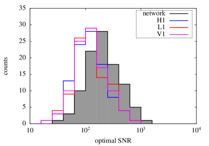
Figure 1: The distribution of SNRs for the open and closed simulated signals.

• GW strain amplitude $h_{0}$: For a given signal with pre-selected $\cos{\iota}$ and $\psi$, a value of $h_{0}$ is chosen to be consistent with the 3-detector multi-IFO optimal SNR having been drawn from a log-normal distribution with parameters $\mu=\log{200},\sigma=0.7$. The optimal SNR$=(h|h)$, where $h$ is the signal (multi-IFO) timeseries and $(x|y)$ is the usual scalar product (see Prix (2007) for a derivation). These parameters define the mean and standard deviation of the SNR natural logarithm. The distribution of SNRs is shown in Figure 1. The SNR distribution parameters were originally selected in order to satisfy the requirement that the weakest searches would detect $\mathcal{O}(5)$ signals and that the strongest would fail to detect approximately the same fraction. Tuning was performed prior to the MDC to establish the distribution parameters based on the original 4 pipelines only (excluding CrossCorr).

Table 3: Signal parameters for the closed part of the MDC.

index	band (Hz)	$f_{0}$ (Hz)	$a\sin i$ (sec)	$P$ (sec)	$T_{\text{asc}}$ (GPS sec)	$h_{0}$ ($10^{-25}$)	$\cos{\iota}$	$\psi$ (rads)	$\phi_{0}$ (rads)
1	50–55	54.498391348174	1.379519	68023.673692	1245967666.024	4.160101	-0.611763	0.656117	4.184335
2	60–65	64.411966012332	1.764606	68023.697209	1245967592.982	4.044048	-0.573940	4.237726	5.263431
3	70–75	73.795580913582	1.534599	68023.738942	1245967461.346	3.565197	0.971016	1.474289	4.558232
5	90–95	93.909518008164	1.520181	68023.681326	1245966927.931	1.250212	-0.921724	0.459888	5.442296
11	150–155	154.916883586097	1.392286	68023.744190	1245967559.974	3.089380	0.323669	1.627885	3.402987
14	180–185	183.974917468730	1.509696	68023.755607	1245967551.047	2.044140	0.584370	3.099251	5.420183
15	190–195	191.580343388804	1.518142	68023.722885	1245967298.451	11.763777	0.028717	5.776490	1.844049
17	210–215	213.232194220000	1.310212	68023.713119	1245967522.541	3.473418	0.082755	5.348830	2.848229
19	230–235	233.432565653291	1.231232	68023.686054	1245967331.136	6.030529	0.224890	1.467310	0.046980
20	240–245	244.534697522529	1.284423	68023.742615	1245967110.972	9.709634	-0.009855	3.008558	1.414107
21	250–255	254.415047846878	1.072190	68023.753262	1245967346.405	1.815111	0.292830	0.302833	0.449571
23	270–275	271.739907539784	1.442867	68023.685008	1245967302.288	2.968392	-0.498809	1.367339	3.578383
26	300–305	300.590450155009	1.258695	68023.687437	1245967177.469	1.419173	0.817770	6.028239	0.748872
29	330–335	330.590357652653	1.330696	68023.774609	1245967520.825	4.274554	0.711395	4.832193	3.584838
32	360–365	362.990820993568	1.611093	68023.714448	1245967585.560	10.037770	0.295336	2.372268	1.281230
35	390–395	394.685589797695	1.313759	68023.671480	1245967198.049	16.401523	0.491537	4.023472	4.076188
36	400–405	402.721233789014	1.254840	68023.628720	1245967251.346	3.864262	0.210925	2.195660	1.662426
41	450–455	454.865249156175	1.465778	68023.695320	1245967225.750	1.562041	-0.366942	2.712863	4.785230
44	480–485	483.519617972096	1.552208	68023.724831	1245967397.861	2.237079	-0.889314	3.754288	5.584973
47	510–515	514.568399601819	1.140205	68023.714935	1245967686.805	4.883365	-0.233705	3.645842	5.773243
48	520–525	520.177348201609	1.336686	68023.634260	1245967675.302	1.813016	-0.241020	0.816681	2.908419
50	540–545	542.952477491471	1.119149	68023.750909	1245967927.484	1.092771	0.939190	4.031313	1.527390
51	550–555	552.120598886904	1.327828	68023.741431	1245967589.535	9.146386	0.120515	3.280902	0.382047
52	560–565	560.755048768919	1.792140	68023.831850	1245967377.203	2.785731	0.486566	4.530901	4.726265
54	590–595	593.663030872532	1.612757	68023.722670	1245967624.534	1.517530	-0.819247	5.029020	0.539005
57	620–625	622.605388362863	1.513291	68023.736515	1245967203.215	1.576918	0.402573	3.365393	5.634876
58	640–645	641.491604906276	1.584428	68023.683124	1245967257.744	3.416297	0.149811	0.273787	5.120474
59	650–655	650.344230698489	1.677112	68023.696004	1245967829.905	8.834794	0.497028	3.148233	3.305762
60	660–665	664.611446618250	1.582620	68023.623412	1245967612.309	2.960648	0.825769	5.828391	6.093132
61	670–675	674.711567789201	1.499368	68023.712738	1245967003.318	6.064238	0.047423	3.616627	6.236046
62	680–685	683.436210983289	1.269511	68023.734889	1245967453.966	10.737497	-0.070857	6.155982	3.343461
63	690–695	690.534687981171	1.518244	68023.681037	1245967419.389	1.119028	-0.630799	2.583073	4.573909
64	700–705	700.866836291234	1.399926	68023.663565	1245967596.121	1.599528	0.052755	0.493210	0.457488
65	710–715	713.378001688688	1.145769	68023.749146	1245967094.570	8.473643	0.420557	1.782869	5.600087
66	730–735	731.006818153273	1.321791	68023.713215	1245967576.493	9.312048	0.596321	4.560452	5.114716
67	740–745	744.255707971300	1.677736	68023.702943	1245967084.297	4.579697	0.028568	3.060388	2.536793
68	750–755	754.435956775916	1.413891	68023.738717	1245967538.698	3.695848	-0.401291	4.343783	0.034602
69	760–765	761.538797037770	1.626130	68023.662519	1245966821.545	2.889282	0.102754	3.302613	3.405741
71	800–805	804.231717847467	1.652034	68023.792724	1245967156.547	2.922576	-0.263274	2.526713	5.884348
72	810–815	812.280741438401	1.196485	68023.718158	1245967159.077	1.248093	0.591815	2.341322	4.708392
73	820–825	824.988633484129	1.417154	68023.683539	1245967876.831	2.443983	-0.169611	0.114125	1.081173
75	860–865	862.398935287248	1.567026	68023.746169	1245967346.324	7.678400	0.432360	0.574140	0.813485
76	880–885	882.747979842807	1.462487	68023.621227	1245966753.240	3.260143	0.447011	5.242454	0.560221
79	930–935	931.006000308958	1.491706	68023.642700	1245967290.057	4.680848	0.015637	5.686775	0.729836
83	1080–1085	1081.398956458276	1.198541	68023.740103	1245967313.935	5.924668	0.121699	3.760452	6.032308
84	1100–1105	1100.906018344283	1.589716	68023.763681	1245967204.150	11.608892	-0.571199	2.310229	2.956547
85	1110–1115	1111.576831848269	1.344790	68023.748155	1245967049.350	4.552730	0.069526	0.365444	2.048360
90	1190–1195	1193.191890630547	1.575127	68023.773099	1245966914.268	0.684002	-0.900467	0.195847	0.873581
95	1320–1325	1324.567365220908	1.591685	68023.703242	1245967424.756	4.293322	0.687636	4.543767	4.301401
98	1370–1375	1372.042154535880	1.315096	68023.760793	1245966869.917	5.404060	-0.080942	4.895973	3.760856

The participants of the challenge were given the following additional information to guide them in the analysis of the data:

• A list of the 5–Hz frequency bands that contain open signals or closed signals. The exact signal parameters for the open signals were also known.

• Participants were required to assume that signals do contain phase contributions due to spin wandering (although they do not). They were to assume that this wandering would have the characteristics of a time-varying spin frequency derivative of maximum amplitude $10^{-12}$ Hz$\cdot$s^-1 with variation timescale $10^{6}$ seconds.

The participants were requested to provide the following data products from their analysis, in order to perform like-for-like comparisons between pipelines:

• Detectability: for the 50 closed signals, identify each as a detection or non-detection. Signal detection is defined as candidates recovered at a confidence equivalent to a $p$-value $=10^{-2}$ accounting for multiple-trials over each 5–Hz band. The $p$-value is generically defined as the probability of obtaining a given detection statistic from data containing only the non-astrophysical background noise.

• Parameter estimation: If a signal is claimed as detected in a given 5–Hz frequency band, then the analysis pipeline must report on the measured signal parameters and associated uncertainties. Note that each individual pipeline has different abilities to measure signal parameters. In particular, no participating pipeline currently provided estimates of $\cos{\iota}$, $\psi$, or $\phi_{0}$.

• Upper limits: for those 5–Hz frequency bands where a signal is not detected, then the pipeline must report the $95$% confidence level upper limit on the GW amplitude $h_{0}$ (also accounting for the multiple trials).

Additional, less-strict instructions were also suggested to participants and included the sensible use of costly computational resources. This was stated so as to be able to compare pipelines under the assumption of broadly similar computational costs. Limiting each pipeline to identical total computational resources is currently an unfeasible restriction to enforce.

V.1 Search Implementations

In this section, a description is given of the different choices made by each search pipeline specifically for this MDC.

V.1.1 Polynomial

For this MDC, the Polynomial search analyzed $1.81\times 10^{6}$ s of simulated data from the LIGO H1 (Hanford) interferometer, spread over a period of $4.855\times 10^{6}$ s, starting at the Global Positioning System (GPS) time $1251698492$. The length of the period was a compromise between sensitivity and use of computational resources. Only $10^{4}$ s long segments of data (without gaps) were analyzed. The data was taken from the interval that had the largest duty cycle in terms of uninterrupted SFT-size segments.

For an all-sky search, Polynomial Search uses 1200 s SFTs, in order to be sensitive to a wide range of binary orbital periods. Since the binary period of Sco X-1 is known, the SFT length can be increased to up to one fourth of its period. If beam patterns were constant in time, the sensitivity would scale with the square root of the SFT length. However, for longer SFTs, evolution of the beam patterns negatively affect sensitivity. $10^{4}$ s was chosen as a compromise.

In total, 50 regions of 5 Hz each were searched, with template parameters in the range $\pm 4.0\times 10^{-5}$ Hz s^-1 for the first derivative of signal frequency with respect to time and $\pm 1.0\times 10^{-8}$ Hz s^-2 for the second derivative with respect to time. The largest expected values of these derivatives assuming 1–$\sigma$ uncertainties on the simulated signal parameters are $\pm 2.1\times 10^{-5}$ Hz s^-1 and $\pm 1.9\times 10^{-9}$ Hz s^-2, respectively.

Detection statistics were determined for each 0.5 Hz frequency bin based on the number of SFTs in which one or more templates exceed the correlation threshold. The threshold required to attain a 1% false alarm probability was determined from the analysis results in a 5 Hz reference band of the MDC data known not to contain a signal (720–725 Hz).

V.1.2 Radiometer

The Radiometer search used all data from H1, L1, and V1 that was coincident between pairs of detectors. This was $\sim$185 days for H1–L1, $\sim$244 days for H1–V1, and $\sim$185 days for L1–V1.

For each 0.25 Hz band the $p$-value was calculated under the assumption that the corresponding $Y$-estimate (see (5)) is Gaussian distributed, as expected from the central limit theorem for the many independent segments. This assumption has been shown to be robust in studies with realistic data Abbott et al. (2007a, 2011). The single trial $p$-value is given by

$$p=\frac{1}{2}\left(1-\operatorname{erf}\left(\frac{{\rm SNR}}{\sqrt{2}}\right)\right)$$ (15)

from which the multi-trial $p$-value is computed via

$$p_{\rm multi}=1-(1-p)^{N}$$ (16)

where ${\rm SNR}=\hat{Y}_{\rm tot}/\sigma_{\rm tot}$ and $N$ is number of independent trials which, for a 5 Hz band with 0.25 Hz bins, is 21 (due to choice of bin start frequency, the Radiometer search here searched slightly beyond the 5 Hz band which resulted in 21 rather than 20 trials). The Radiometer search results were converted to match the format presented in this paper. The conversion process is described in Appendix B.

V.1.3 Sideband

The Sideband search analyzed a 10-day stretch of MDC data (864000 sec) using all 3 interferometers and with an initial GPS time of 1245000000. This was not an optimally selected 10-day stretch of data (as was done in the Aasi et al. (2014b)), with the duty factors for the three interferometers being $70\%$, $58\%$ and $80\%$ for H1, L1 and V1 respectively. Since the noise floor is constant in time, optimality in this case is dependent upon the duty factors of the data combined with the diurnal time variation of the antenna patterns in relation to the Sco X-1 sky position. The “optimal” 10–day data-stretch has subsequently been identified as starting at GPS time 1246053142 and having duty factors $86\%$, $83\%$ and $94\%$.

For Gaussian noise, each value of the $\mathcal{C}$-statistic is drawn from a central $\chi^{2}_{4M}$ distribution, where $M=2{\rm ceil}(2\pi f_{0}a\sin i)+1$ is the number of sidebands. For $N$ independent trials, $p$-values are therefore calculated as

$$p=1-\left[F\left(\mathcal{C},\,4M\right)\right]^{N},$$ (17)

where $F(\mathcal{C},4M)$ is the cumulative distribution function of a $\chi_{4M}^{2}$ distribution evaluated at $\mathcal{C}$. If one assumes each trial is statistically independent and defines a target false alarm probability, (17) allows us to determine a threshold value of the maximum recovered $\mathcal{C}$-statistic, denoted $\mathcal{C}^{*}_{N}$ (for details see  Aasi et al. (2014b)). In practice, there is strong correlation between $\mathcal{C}$-statistic values due to the nature of the comb template. In addition there are small deviations from the expected statistical behavior of the $\mathcal{C}$-statistic due to approximations and noise normalization procedures within the search algorithm. Therefore, Monte Carlo simulations have been used to identify a correction to $\mathcal{C}^{*}_{N}$ that corresponds to the desired false alarm probability. The corrected threshold statistic is given by

$$C^{\star}_{\kappa}=C^{\star}_{N}\left(1+\kappa\right)-4M\kappa,$$ (18)

where $\kappa=0.3$ Aasi et al. (2014b). A detection is therefore claimed if the maximum recovered value of the statistic satisfies $\mathcal{C}>\mathcal{C}^{\star}_{\kappa}$.

V.1.4 TwoSpect

The TwoSpect pipeline analyzed all MDC data from each interferometer separately. For each interferometer, detection statistics and corresponding single-template $p$-values were computed for each template. A set of most significant $p$-value outliers in 5 Hz bands were produced for each interferometer, subject to a $p$-value threshold inferred from Monte-Carlo simulations in Gaussian noise (see a forthcoming methods paper Meadors et al. (2015) for details). These sets were compared in pairwise coincidence (H1-L1, H1-V1, or L1-V1), where coincidence required proximity within a few grid points in the parameter space. Surviving outliers were classified as a detection at the predefined 1% false alarm threshold.

In the case of detection, the highest $p$-value from a single interferometer in a given band was used to produce estimated signal parameters. Uncertainties in these parameters were determined from the open signals within the MDC. For the intrinsic signal frequency and modulation depth, we estimated the mean and standard deviation of parameter estimation error in the open signals. This error varied little for different injected signal strength $h_{0}$, so function was or could be estimated to yield more precise uncertainty measurements other than the mean error. Since the parameter distribution for the closed signals was known to be the same as the open signals, we reported the mean error as our estimate of uncertainty. Since some higher-frequency bands appeared to have greater error, a seperate mean error was estimated for those bands. Further details to be reported in a forthcoming methods paper. Confidence intervals calculated more rigorously for the signal amplitude. Upper-limits on signal amplitude were determined from an estimate of the 95% confidence level of non-detected open MDC signals. The largest uncertainty in upper limits and signal amplitude estimation derives from the ambiguity between true $h_{0}$ signal and $\cos\iota$ inclination. This ambiguity cannot be resolved with the present algorithm and depends partially on the assumed prior distribution of signal ampltitudes; the uncertainty was estimated by simulation. Complete details of the parameter estimation and upper-limit setting procedure are detailed in the methods paper Meadors et al. (2015).

V.1.5 CrossCorr

The CrossCorr pipeline analyzed all MDC data from all three interferometers together, calculating cross-correlation contributions from each pair of SFTs for which the timestamps differed by less than a coherence time $T_{\text{max}}$. In order to control computational costs, different values of $T_{\text{max}}$ were used for bands in different frequency ranges, and also for different parts of orbital parameter space within each frequency band, as detailed in Appendix D. Each 5 Hz frequency band was divided into 100 frequency slices and eight regions of orbital parameter space, described in more detail in Section D.1. The resulting 800 parameter space regions were then searched using a cubic lattice with a metric mismatch of $0.25$ (as defined in Whelan et al. (2015)), and the highest resulting statistic values combined into a “toplist” for the entire band. Local maxima over parameter space were in principle considered as candidate signals, although in practice each band contained high statistic values clustered around a single global maximum.

A “refinement” was performed around each such maximum, decreasing the grid spacing by a factor of 3 and limiting attention to a cube 13 grid spacings on a side. The resulting maximum statistic value was high enough to declare a confident signal detection for each of the 50 bands, but for some of the weaker detected signals, a followup was performed with an even finer parameter space resolution and a longer coherence time, which approximately doubled the statistic value.

Since the CrossCorr statistic is a sum of contributions from many SFT pairs, and is normalized to have unit variance and zero mean in the absence of a signal, the nominal significance of a detection can be estimated using the cumulative distribution function of a standard Gaussian distribution. A false alarm probability for the loudest statistic value in a 5 Hz band can be estimated by assuming that each of the templates in the original grid was an independent trial and multiplying the single-template $p$-value by the associated trials factor. The $p$-values generated by this procedure are not reliable false alarm probabilities, however, since with typical trials factors of $10^{8}$, the relevant single-template $p$-values are $10^{-10}$ or smaller, for which the Gaussian distribution is no longer a good approximation. Therefore, the nominal multi-template $p$-value corresponding to an actual false alarm probability of 1% was estimated by running the first stage of the pipeline on forty-nine 5 Hz bands containing no signal. Comparing this value to those associated with the detected closed signals showed the latter all to be detections. For more details, see Section D.2 of Appendix D.

For each detected signal, the best-fit values of $f_{0}$, $a\sin i$ and $T_{\text{asc}}$ were determined by interpolation, fitting a multivariate quadratic to the 27 statistic values in a cube centered on the highest value in the final grid, and reporting the peak of this function. Parameter uncertainties were a combination of: residual errors from the interpolation procedure, statistical errors associated with the noise contribution to the detection statistic, and a systematic error associated with parameter offset associated with the unknown value of $\cos\iota$. Additionally, analysis of the open signals showed a small unexplained frequency-dependent bias in the $a\sin i$ estimates. To produce conservative errorbars, the size of the empirical correction for this bias was added in quadrature with the other errors. The procedure is described in further detail in Appendix D and Zhang et al. (2015).

VI Results

Participants in the MDC were asked to submit their results on the 50 closed signals no later than 30 April 2014 in the form described in Table 4. Four pipelines (Polynomial, Radiometer, Sideband and TwoSpect) completed their analysis of the closed signals on or near the original deadline of the MDC, at which point the previously secret parameters were made available. Some of the final post-processing analyses took place after the initial submissions in order to provide the full final submission. A fifth analysis method, the CrossCorr pipeline, was not in place soon enough to participate in the original challenge, but carried out a subsequent opportunistic analysis. This “self-blinded” analysis was conducted and a submission table prepared without looking at the parameters of the closed signals. Table 5 summarizes these submission dates.

From the submission tables of each pipeline, we have generated a number of comparison figures and tables. The description of results are divided into the topics of detection, upper-limits and parameter estimation.

Table 4: The MDC submission parameters.

parameter	symbol	units	description
PULSAR INDEX			the index of the closed pulsar	}53mmfor all signals
PULSAR FSTART		Hz	the lower bound on the search frequency band
PULSAR FEND		Hz	the upper bound on the search frequency band
DETECTION			please state either yes or no
P VALUE	$\log{p}$		natural-log of the multi-trial statistical significance of the loudest event found
H0 UL	$h_{0}^{95\%}$		95% confidence upper limit on $h_{0}$, the dimensionless strain tensor amplitude	}23mm for non-detected signals only
H0 EST	$h_{0}$		best estimate for $h_{0}$, the dimensionless strain tensor amplitude	}103mm for detected signals only
H0 ERR	$\Delta h_{0}$		uncertainty on the best estimate of $h_{0}$
F0 ESTIMATE	$f_{0}$	Hz	best estimate for $f_{0}$, the intrinsic GW frequency
F0 ERROR	$\Delta f_{0}$	Hz	uncertainty on the best estimate of $f_{0}$
ASINI EST	$a\sin i$	sec	best estimate for the product of the orbital radius and the sin of the inclination
ASIN ERR	$\Delta(a\sin i)$	sec	uncertainty on the best estimate of $a\sin i$
PERIOD EST	$P$	sec	best estimate for the orbital period
PERIOD ERR	$\Delta P$	sec	uncertainty on the best estimate of $P$
TASC EST	$T_{\text{asc}}$	GPS sec	best estimate for the time of ascension
TASC ERR	$\Delta T_{\text{asc}}$	GPS sec	uncertainty on the best estimate of the time of ascension

Table 5: Dates of submitted results for the MDC.

Submission deadline 30 April 2014	TwoSpect	Polynomial	Radiometer	Sideband	CrossCorr
Initial submission	30 April 2014	1 May 2014	1 May 2014	19 May 2014	19 Dec. 2014
Final submission	22 Aug. 2014	1 Oct. 2014	29 Mar. 2015	27 June 2014	16 Jan. 2015

VI.1 Detection

An overview of the detectability of the MDC signals is shown in Figure 2. The list of specific signals detected by each pipeline are given in Appendix A. Three different figures of merit are plotted: the detection success as a function of $h_{0}$, as a function of optimal SNR, and as a function of reported $\log_{10}(p)$. Of the original four pipelines that ran in the MDC (see Table 5), TwoSpect was able to detect the most signals and detect signals of lower intrinsic strain and SNR than the other three pipelines. The CrossCorr pipeline, which ran an opportunistic, “self-blinded” analysis in the months following the original MDC, was able to detect all 50 signals.

Specifically, the CrossCorr, TwoSpect, Radiometer, Sideband, and Polynomial pipelines detect 50, 34, 28, 16, and 5 respectively with ratios of 1, 1.83, 3.27, 5.21, and 11.2 between the weakest detected $h_{0}$ values from each pipeline and the weakest signal present. Equivalent ratios in detectable optimal SNR are 1, 2.0, 2.2, 4.1, and 7.0. We also plot the estimated value of the $\log_{10}(p)$, the (base 10) logarithm of the $p$-value as defined in Section V, for all signals (detected and non-detected) in the third panel of Figure 2.

Among the four original pipelines, we note that all detected signals from the Polynomial pipeline are a subset of those detected by the Sideband pipeline which in turn are a subset of those detected by the Radiometer pipeline which, with the exception of pulsar 52, are a subset of those detected by TwoSpect.(TwoSpect saw an above-threshold statistic in the pulsar 52 band for V1, but not in coincidence with H1 or L1, so no detection was declared). While the CrossCorr pipeline was the most successful, detecting all 50 closed signals, it is also the least mature. In particular CrossCorr has not yet been used for an astrophysical analysis of GW detector data as TwoSpect, Sideband and Radiometer have, and its behavior in the face of non-Gaussianity and other instrumental noise features has not been probed by this idealized MDC.

Due to the relatively low number of simulated signals in the MDC we are aware that we do not deeply probe the interesting boundaries in sensitivity between pipelines. In particular, the closed signal detections give no indication of the lower limit of detectability for the CrossCorr pipeline. Some insight can be taken from the open signal data, in which CrossCorr was able to find 49 of the 50 open signals. The one “missed” signal had $h_{0}=3.81\times 10^{-26}$ and an optimal SNR of $33$. The “quietest” of the 49 open signals which CrossCorr detected had $h_{0}=4.96\times 10^{-26}$ and an optimal SNR of $48$. For comparison, the weakest of the closed signals were pulsar 90 with $h_{0}=6.84\times 10^{-26}$ and pulsar 64 with an optimal SNR of $71$.

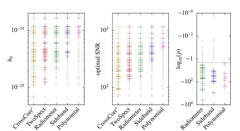
Figure 2: A comparison of detected signal properties for each search pipeline. We plot the values of $h_{0}$, optimal SNR, and estimated $\log_{10}(p)$ value for the detected (color) and non-detected (grey) signals from each pipeline. The 3rd panel shows the $\log_{10}(p)$ values from the search pipelines which were able to estimate reliable values, with the black horizontal dashed line representing the detection threshold of $\log_{10}(p)=-2$. Note that the TwoSpect and CrossCorr pipelines generated nominal $p$-values, but as they were known not to be quantitatively accurate, they are not shown here. Note also that the CrossCorr pipeline obtained results seven months beyond the original deadline for the MDC, as detailed in Table 5. The full list of detected and non-detected signals is given in Appendix A

Further comparison between pipelines is shown in Figure 3 where detection efficiency versus the GW strain $h_{0}$, and the optimal SNR respectively are plotted. Detection efficiency is defined as the fraction of signals claimed as detected at the chosen confidence ($p<10^{-2}$) as a function of the value indicated on the $x$-axis. For example, the Sideband search achieves a detection efficiency of $\approx 0.8$ at $h_{0}=7\times 10^{-25}$. The efficiency curves and their uncertainties are obtained by marginalizing over the parameters of a basic sigmoid function using the posterior distribution generated from the 50 detection/non-detection results from the closed signal bands. (Note that although the CrossCorr pipeline detected all 50 signals, the Jeffreys prior used for the sigmoid parameters prevents the posterior from implying 100% efficiency at all signal strengths, as it would with a maximum likelihood method. The inferred sigmoid parameters for CrossCorr are still somewhat arbitrary and dependent on this choice of prior, however.) At 50% detection efficiency, the scaling in $h_{0}$ sensitivity relative to the weakest signal in the closed data set is $\approx$0.40, 3.4, 4.6, 7.9, and 13 for CrossCorr, TwoSpect, radiometer, sideband and polynomial, respectively. In terms of SNR at 50% efficiency, these numbers are $\approx$0.44, 2.2, 2.8, 4.4, and 7.0.

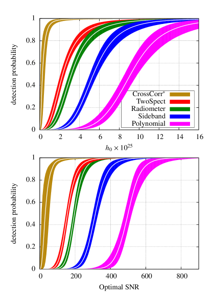
Figure 3: The upper and lower plots show the detection efficiencies for each pipeline as a function of $h_{0}$ and multi-detector optimal SNR respectively. The shaded regions represent the 50% uncertainty (inter-quartile range) after marginalizing over the parameters of a basic sigmoid function $f(x)=(1+e^{-\alpha(\log(x)-\beta)})^{-1}$ using the posterior distribution generated from the 50 detection/non-detection results from the closed signal bands. The posterior was constructed using a Jeffreys prior on $\alpha$ and $\beta$ so that the inferred efficiencies are all less than unity, even for the CrossCorr pipeline (whose results were obtained in self-blinded mode several months after the others and half a year beyond the nominal end date of the MDC, as detailed in Table 5), which detected all 50 closed signals. However, the exact turnover point of the CrossCorr efficiency curve is more uncertain and less robust against changes of the fitting procedure than the others.

VI.2 Parameter Estimation

The parameter estimation abilities of each pipeline are varied and range from the minimum state of inference: only estimating the signal frequency, up to the maximum state: estimation of frequency, orbital semi-major axis and time of ascension, and the strain amplitude. None of the pipelines performed additional parameter inference on $\cos\iota,\psi$ or $\phi_{0}$. None treated the orbital period as a search parameter and hence they do not refine this estimate beyond the initial known prior distribution. There was only very limited candidate follow-up analyses to potentially enhance parameter estimation via, e.g., analysis of additional data, or deeper analysis over localized parameter space regions around candidates. (CrossCorr employed a limited narrow-parameter-band analysis with a longer coherence time on three of the quietest detections. This method was developed to confirm marginal detections and was used for that purpose on one of the open signals. While it was not necessary for the closed-signal detections, it did provide more accurate parameter estimates as well as more confident detections, and could in principle have been used more widely.) The details of the estimated parameter values from all pipelines can be found in Appendix A.

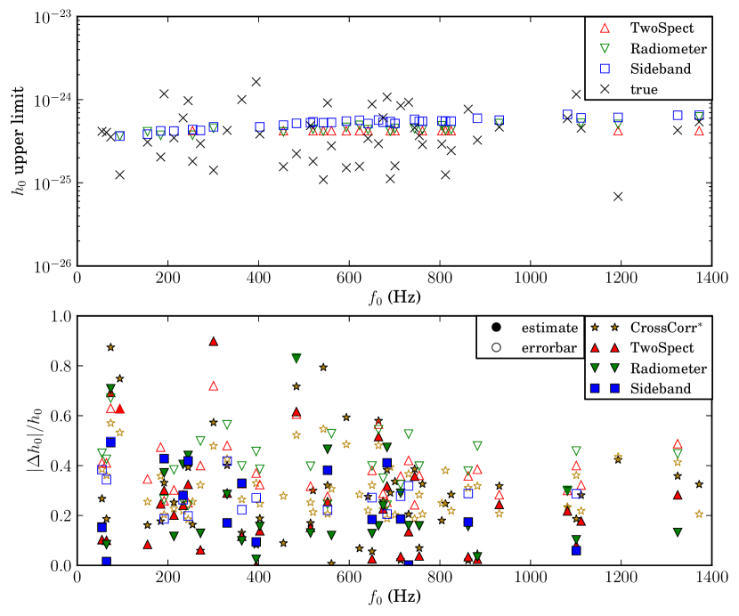
Figure 4: Comparison of signal amplitude estimates (from detected signals) and upper limits (from non-detected signals) from each pipeline as a function of intrinsic signal frequency. The top panel shows the $95\%$ confidence upper-limits on $h_{0}$ for non-detected signal from each pipeline that provided such results. The black crosses indicate the true value of $h_{0}$. In the bottom panel, the solid symbols in the top panel show the fractional errors in $h_{0}$ estimates, and open symbols show the quoted one-sigma errorbars, again divided by the true $h_{0}$ value. The uncertainty in $h_{0}$ is comparable for all pipelines which provided estimates, since all were dominated by the unknown value of $\cos\iota$. The complete details of the amplitude estimates and upper limits can be found in Appendix A.

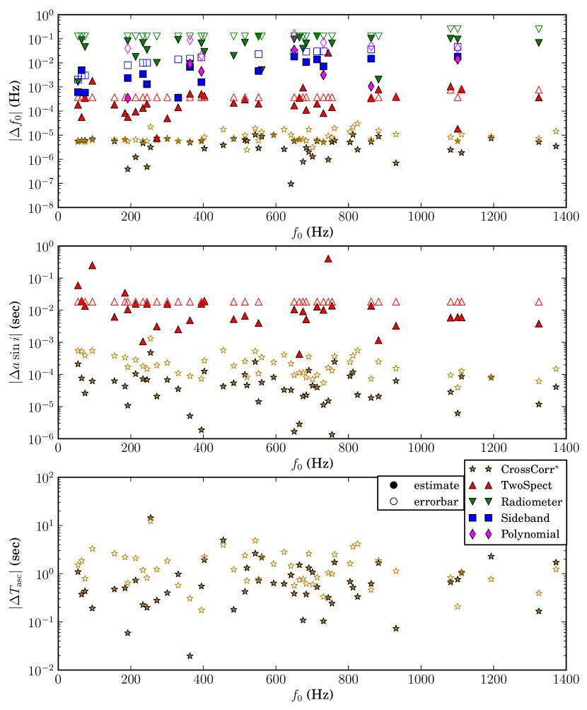
Figure 5: Comparisons of parameter estimation for detected signal from each pipeline as a function of intrinsic signal frequency. The solid symbols in each plot show the difference between the true and estimated values of intrinsic signal frequency, projected semimajor axis, and time of passage of the ascending node for the detected signals for pipelines which report those quantities. The open symbols show the quoted one-sigma errorbars corresponding to each estimate. The complete details of the parameter estimates can be found in Appendix A. The causes of notable outliers seen in the estimation of the orbital semi-major axis by TwoSpect are discussed in Section VI.2.

Figure 4 shows the fractional error in the estimates of $h_{0}$, along with the quoted errorbars, for the detected signals and the upper-limits set for those signals not detected. Note that the TwoSpect pipeline sets a fixed upper-limit value for each non-detected signal at the level of $4.23\times 10^{-25}$, and the Polynomial pipeline does not produce estimates or upper-limits for $h_{0}$. (The CrossCorr pipeline detected all 50 signals and therefore had no upper limits to report.) It is clear that for non-detections, there is very little spread between pipelines in the resulting upper-limits. Typically, these values vary between pipelines by of order of tens of percent with TwoSpect and the Radiometer searches consistently setting the most stringent upper-limits. As can be seen from the second panel in Figure 4, in all cases for detected signals, the estimated $h_{0}$ values are consistent with the true values given each pipeline’s reported uncertainties. Additionally, the $h_{0}$ uncertainties are comparable for all pipelines. This is because these searches are all sensitive not to $h_{0}$ but to a combination of $h_{0}$ and $\cos\iota$ known as $h_{0}^{\text{eff}}$ and given by

$$(h_{0}^{\text{eff}})^{2}=h_{0}^{2}\,\frac{[(1+\cos^{2}\iota)/2]^{2}+[\cos\iota]^{2}}{2}$$ (19)

This is equal to $h_{0}^{2}$ for circular polarization ($\iota=0^{\circ}$ or $180^{\circ}$) and $\frac{h_{0}^{2}}{8}$ for linear polarization ($\iota=90^{\circ}$), and has an average value of $\frac{2}{5}h_{0}^{2}$ when averaged isotropically over the inclination angle $\iota$. The uncertainty in the value of $\cos\iota$ dominates the other measurement errors for $h_{0}$ in each of the pipelines.

The first panel of Figure 5 gives the difference between the true and estimated intrinsic GW frequency. Note that for search frequencies below $\sim$1 kHz, the Radiometer search returns a fixed estimate for frequency uncertainty of $\pm 0.125$ Hz based on the size of the frequency bins used in the Radiometer analysis. Beyond this frequency, where the signal is likely to span two frequency bins, the uncertainty is increased to $\pm 0.25$ Hz. These uncertainties are conservative. In all but 1 case, the Radiometer analysis correctly identifies the signal frequency bin. For pulsar 65, two adjacent bins yielded $p$-values below the detection threshold and the lower of the two was selected as the candidate signal. The true signal location, however, was within the rejected bin. The TwoSpect search has the best frequency accuracy of the original four pipelines of the MDC, and in the majority of cases is consistent with the true values to within their quoted error bars. There is one notable outlier, however, for a low-SNR detection. The Sideband search’s claimed uncertainties are conservative and appear to have overestimated uncertainties since all 18 detected signals lie within the 1-$\sigma$ error bars. The Polynomial search frequency estimates are consistent within its estimated uncertainties with the true values for all 7 of its corresponding detected signals. The CrossCorr search produces considerably smaller error bars than all of the original 4 MDC pipelines, and the errors in its frequency estimates are consistent with those uncertainties. CrossCorr’s parameter space precision is due in part to its method of finding the best fit parameters by interpolation rather than reporting the grid point with the highest statistic value.

The final two panels of Figure 5 represent the orbital parameter estimation ability of the TwoSpect and CrossCorr pipelines. These two searches reported the projected orbital semi-major axis, while CrossCorr was the only pipeline to estimate the time of ascension $T_{\text{asc}}$. The interpolation performed by CrossCorr allows it to obtain parameter estimates with smaller error bars, with a resolution finer than its final grid spacing. For TwoSpect, of the majority of signals that are detected, the $a\sin i$ estimate is consistent with the true values and uncertainties are $\mathcal{O}(0.02)$ s (representing a $\approx$1.5% error). This indicates a potential improvement over the known prior observational uncertainty by a factor of ${\sim}$10. There are however, 2 notable outliers in which $a\sin i$ is significantly underestimated. This occurs when a strong signal in one detector matches a weak signal in another; reading parameters off the highest $p$-value template does not always yield an accurate estimate in this marginal case. Further refinement of coincident parameter estimation, or parameter estimation in a future coherent mode, may correct this problem.

In Figure 6, distributions of parameter estimation offsets from the true values and rescaled by the estimated measurement uncertainty are shown. It is expected to observe distributions that are proportional to zero mean, unit variance, Gaussian distributions. For the estimates of the signal strain amplitude $h_{0}$ for which we have results from four algorithms, the distributions are generally consistent with the expected Gaussian. This is also the behavior for the estimates of $a\sin i$ from the TwoSpect algorithm, although it should be noted that 2 outliers (visible in the middle panel of Figure 5) have been omitted from this plot. The $a\sin i$ errorbars reported by CrossCorr appear to be somewhat larger than the typical actual offsets, which is to be expected from the inclusion of the bias correction as a conservatively-estimated source of error. For the intrinsic GW frequency estimation, deviations are observed from the expected behavior for the Sideband, Polynomial, and Radiometer approaches whereas the TwoSpect and CrossCorr algorithms are broadly consistent with expectations. In all cases, matching the expectations means that one can infer that the 1–$\sigma$ uncertainty estimates are valid. For the Polynomial, Sideband, and Radiometer frequency results, there is an apparent bias towards overestimation of the 1–$\sigma$ errors (this is expected in the case of the Radiometer). It should be noted that in the Polynomial case, there are only seven detected signals from which the distribution can be constructed and hence these results are subject to large statistical uncertainties.

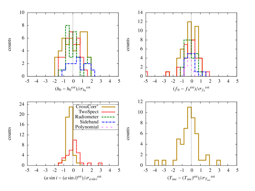
Figure 6: Distributions of estimated parameter offsets relative to their estimated measurement uncertainties for the detected MDC signals. Only TwoSpect and CrossCorr return an estimate of the projected semimajor axis, and only CrossCorr returns an estimate of time at the ascending node. None of the pipelines return period estimates.

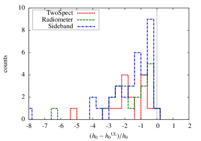
Figure 7: Distribution of offsets between $h_{0}$ upper limits and actual values non-detected MDC signal. The polynomial search returns only frequency estimation for detection and does not return an $h_{0}$ upper-limit, while CrossCorr had no non-detections among the 50 closed signals.

For the Sideband frequency estimates, a narrow distribution is obtained implying that the algorithm produces overly conservative uncertainties. This is expected due to the difficulty of converting the intrinsically multi-modal Sideband detection statistic into an equivalent single-mode uncertainty. In the limit of high SNR, the maximum Sideband detection statistic is expected to belong to the frequency bin coincident with the true intrinsic GW frequency. This frequency bin has a relatively narrow width in comparison to other algorithms and is given by $\approx 1/T$ where $T$ is the length of the observation (so in this case $\sim 10^{-6}$ Hz). For lower SNR (still detectable signals), the maximum could originate from Sideband statistics from integer multiples of $\pm 1/P$ Hz away from the true value. The total segmented space will contain $\mathcal{O}(10^{-6})$ Hz but for Sco X-1 will span $\mathcal{O}(10^{-4})$ Hz. Based on the range of offsets between the true frequency and those associated with the maximum statistic observed in the open data set a conservative value of $0.042(f/1\,\text{kHz})$ Hz was chosen for the error on frequency.

In Figure 7, the distribution of $h_{0}$ upper-limit offsets relative to the true $h_{0}$ value are shown. The expected form of such a distribution is an unknown function of the original SNR distribution of the MDC signals and the search algorithm in question. An expected property of this distribution, however, is that, given a 95% confidence on the upper-limit value, 5% of the quoted values should be greater than the true $h_{0}$ value. Given that each of the 3 algorithms that reported $h_{0}$ upper-limits only did so on a limited number of undetected signals it is expected that $\mathcal{O}(1)$ of the upper limits would lie below the true strain value, which is consistent with observations.

VI.3 Computational cost of the MDC analysis

In one sense it would be desirable to compare each algorithm at fixed computational cost, therefore separating the efficacy of the algorithm from the computing power used. The implicit restriction on computational expense applied to the MDC analysis was limited by the availability of computational resources (equally available to all participants) and the length of the challenge itself.

The current implementations of both the Radiometer and the Sideband searches are not computationally limited. For the Radiometer search this means that choices made in the algorithm design result in the ability to analyze all MDC data over the entire parameter space on a single machine in $O(\text{hours})$. This constitutes a tiny fraction of the available computational power. The post-processing of the results is equally cheap due to the relative insensitivity of the Radiometer in parameter estimation. For this particular MDC much effort through additional, relatively cheap but time consuming injection studies (restricted to the Radiometer analysis) was required to calibrate the Radiometer, designed for stochastic signals, for continuous waves. Future Radiometer implementations will benefit from source-specific tunings which will likely increase the computational cost but will maintain the algorithm status as not computationally limited.

The Sideband search is also not computationally limited. However, this is due to its high sensitivity to spin-wandering and hence there is a self-imposed limit of 10 days observation. The two main search stages can then be run in a $O(10)$ hours using $\sim$100 machines (within a cluster). Post-processing of the results for parameter estimation adds an additional comparable cost. Whilst this is considerably more costly than the Radiometer algorithm, it similarly costs far less than the available computational power.

The Polynomial search is highly computationally limited, primarily due to its design as an all-sky search; the number of templates cannot be reduced substantially using the known parameters available for Sco X-1. Furthermore, the SFT length was increased compared to the all-sky search strategy, which increases sensitivity at the cost of further increasing computation cost. The relative immaturity as an established algorithm may have contributed further to the time required. For this MDC, only 56 days of simulated data from just one of the three available interferometers was analyzed (H1). This allows all potential MDC signals to be analyzed, but at a reduced sensitivity compared to analysis of the full data set. With this, restriction, the computational cost was limited to approximately $10^{6}$ core-hours.

For TwoSpect the MDC search over the 100 signals (open and closed) required $\sim$few weeks of wall-clock processing time using $O(10^{3})$ CPUs. Directed search post-processing was developed as part of the MDC, and the additional cost required was $\sim$few days in total on one CPU. The main tunable algorithmic parameters of TwoSpect in a directed search for Sco X-1 are template spacings for the tested frequency and projected semi-major axis, along with the SFT coherence time. The template spacings were chosen to give a mismatch no greater than 0.20. The SFT length was chosen to be 360 s for higher frequency bands, above 360 Hz, and 840 s for lower frequency bands. These SFTs kept most of the modulated signal frequency contained within one bin per SFT. Ideally, SFTs are as long as possible, just short of where spectral leakage would occur; we chose to restrict ourselves to two sets of SFTs since the cost of generating more would be high for relatively low gains in sensitivity.

As described in Section IV.3, the computational cost for CrossCorr grows with search frequency, but can be tuned by reducing the coherence time $T_{\text{max}}$. To maintain approximately the same computing cost for each signal band, a range of $T_{\text{max}}$ values were used, as listed in Table 12. The total computing cost for the fifty closed signal bands in this setup was approximately $20,\!000$ CPU-days.

VII Discussion

We have considered five search pipelines presently available to the GW community that are capable of searching for the continuous GW emission from Sco X-1. A general overview of each pipeline has been presented with regards to sensitivity, computational efficiency, parameter space dependencies, and parameter estimation capabilities. To compare these methods, an MDC was performed that included 50 unknown simulated signals consistent with the known Sco X-1 parameter space. Each algorithm has presented its results of the 50 signals in terms of detection status and signal parameter estimation in the event of a detected signal exceeding a predefined false-alarm threshold. These results were then used to compare the algorithms and to elucidate unforeseen strengths and weaknesses in each approach. We expect each team will employ improvements to the pipelines in future versions.

Perhaps the most critical figure of merit for each pipeline is the detection efficiency. Among the four original pipelines that ran in the MDC, the clear leader in this category was the TwoSpect algorithm, which detected 34 of the 50 closed signals. The next most sensitive algorithm was the Radiometer search with 28 detections, followed by the Sideband search with 16, and finally the Polynomial approach with 7. The CrossCorr pipeline, which completed its preliminary, self-blinded analysis seven months after the original MDC deadline, as detailed in Table 5 detected all 50 closed signals. The definition for detection in the MDC is less stringent than typically used in continuous GW searches, and, in the presence of non-Gaussian noise (as is usually the case with real GW detectors), a higher threshold would be used. Since the focus of the MDC was on algorithm comparison, this choice acted as a discriminator between pipelines but should not necessarily be used as a true indicator of detectable signal strengths in real data.

Whilst it is difficult in general to rank the algorithms with respect to some measure of sensitivity at fixed computational cost, it is very clear that the Radiometer algorithm does the best with limited computational power. It uses less computational power than the Sideband search and yet claims detection on more signals. In comparison to the TwoSpect and CrossCorr algorithms, which consumed the most computational resources, the Radiometer search detected $82\%$ of the TwoSpect signals and $56\%$ of the CrossCorr signals using $<1\%$ of the computational power of either search.

The weakest signal in this relatively small MDC sample had strain $h_{0}\approx 6.8\times 10^{-26}$ at $1190$ Hz, and the weakest detected by the four pipelines which ran during the original MDC time frame had $h_{0}\approx 1.4\times 10^{-25}$ at $300$ Hz which is slightly greater than the torque-balance limit for Sco X-1 at a GW signal frequency of 50 Hz and almost an order of magnitude higher than the corresponding limit at a GW signal frequency of 1500 Hz. From this perspective it is clear that improvements must be made to these algorithms in order to make detection a possibility and to start to set astrophysically interesting constraints on GW emission from Sco X-1. This is also true of the CrossCorr pipeline, which detected all of the closed signals, but missed one open signal with $h_{0}=3.8\times 10^{-26}$, indicating that its detectability threshold was likely slightly above the torque balance level as well, at least for the coherence times considered in this analysis.

The Sideband search suffers the most from the potential effects of spin-wandering in the Sco X-1 system. This issue has not been considered in this analysis other than to acknowledge its possible effects and to assume, rather than model, its presence. Multiple 10-day data segments can, in principle, be added semi-coherently to improve the sensitivity of the Sideband search Aasi et al. (2014b). Other algorithms will most likely, at some point in their development, have to account for this feature. To do so, we must be able to accurately quantify its realistic behavior and to model it in our simulations. The point at which an algorithm attains a frequency resolution at the level at which spin-wandering is expected to vary is the point at which new data analysis techniques are required. For the Radiometer and Polynomial searches this is unlikely to ever be the case which makes them attractive in their robustness. For CrossCorr, the level of spin wandering described in the MDC is likely to limit the coherence time $T_{\text{max}}$ to about 12 hoursWhelan et al. (2015), which could pose limitations on future searches with even longer coherence times. For TwoSpect the effect requires further study and for the Sideband search, the 10 day observation limit is already a constraint imposed by spin-wandering.

In a realistic search, outliers would typically be further analyzed using different follow-up methods. This can be as simple as analyzing the same set of data using other analysis pipelines to verify the presence of a putative signal, or the follow-up can involve multiple, hierarchical steps to refine and improve the signal-to-noise ratio of a candidate signal.

All of the algorithms presented here have planned improvements for the advanced detector era. It is currently unclear how much the detection sensitivity could improve from each of the analyses. Investigations into the following specific enhancements are already underway.

• TwoSpect: coherently combining SFTs from H1, L1, and V1 prior to the second Fourier transform step should enable improvements in the detectable $h_{0}$. Indeed, initial tests indicate an additional 7 could be detected of the 16 closed signals that were originally missed by TwoSpect. A coherent analysis of the second Fourier transform should also yield non-negligible improvement in detection efficiency as well. It is also possible that a finer grid spacing and/or interpolation could be used to improve the uncertainties in parameter estimates, although the improvement in $f_{0}$ and $a\sin i$ estimation may be limited by noise fluctuations.

• Radiometer: applying a variable-size frequency window rather than fixed $0.25$ Hz bins will improve sensitivity. The width of the window will scale proportionally with frequency and be tuned to the expected modulation depth of the Sco X-1 signal. It will also be overlapped to reduce the chance of mismatch with a possible signal.

• Sideband: Combining the results from multiple short observations (rather than relying on a single short observation) will improve sensitivity. There is also the possibility to perform partial orbital phase demodulation in the coherent $\mathcal{F}$-statistic stage of the analysis. This would take advantage of prior orbital phase knowledge which is currently ignored by all algorithms taking part in this MDC.

• Polynomial: With improved algorithm and implementation efficiency, as well as the use of graphical processor units it will be possible to analyze a larger subset of the data, therefore improving sensitivity. For parameter estimation a secondary search can be launched with smaller template grid spacing to refine the frequency of signal candidates. It may also be possible to use multiple detectors to triangulate a signal and estimate the sky location. This would also enable an estimate of the $h_{0}$ of the GW. Work to extend templates to span multiple coherent intervals is also planned.

• CrossCorr: since the search is computationally limited, the primary planned approach to improve the sensitivity is to increase the speed of the code. Any such increase in speed would allow longer coherence times, and therefore improved sensitivity, at the same computing power. Possible avenues range from reorganization of the computation of weightings related to spectral leakage, to leveraging vectorized hardware instructions such as AVX or SSE (currently employed by the TwoSpect pipeline), to a more fundamental reorganization of the calculation to be performed in the time domain with the “resampling” method defined in Jaranowski et al. (1998); Prix (2011). Enhancements not related to speed may include filtering with multiple templates to make the search sensitive to other combinations of the amplitude parameters besides $h_{0}^{\text{eff}}$.

In addition to the algorithms that took part in this MDC, the stacked $\mathcal{F}$-statistic approach discussed in Section III.6 has great potential to exceed the performance of the five main algorithms presented in this paper. Recent sensitivity estimates published for a hypothetical search with days-long coherence timeLeaci and Prix (2015) are especially encouraging. It should be stressed that this search in development should be compared to the future sensitivities of the existing algorithms. Likewise, the CrossCorr algorithm, which produced the best results on the MDC data included in this paper, had the advantage of running later, so some care should be taken when comparing its results to the four methods run during the MDC timeframe, which have been undergoing enhancements since then. Also, the CrossCorr pipeline is still relatively immature, and its performance on actual interferometer data is yet to be tested.

The work presented here has been a valuable first step towards validating our algorithms, understanding their uncertainties, quantifying our detection criteria (albeit in Gaussian noise), and gauging our best sensitivity to Sco X-1. We intend to build on this work, and at the time of writing this manuscript, are deciding on the format and features of the next MDC. Among other improvements, the three main advancements we plan to make are the addition of spin-wandering to our simulated signals, the inclusion of non-Gaussian noise (most likely, rescaled real 1st generation detector noise), and the use of signal amplitudes at, or below, the torque balance limit. This will constitute a far greater challenge to the participants, but will allow us to transition from primarily comparing our pipelines to being able to make predictions about astrophysically realistic scenarios in the advanced detector era.

Appendix A Complete MDC results

This section contains tables given the complete results of the searches, which are summarized in Section VI. The specific signals detected by each pipeline, summarized in Figure 2 and Figure 3, Figure 6, and Figure 7 are listed in Table 6. (Note that the details of the signals themselves are in Table 3.) The upper limits (for non-detected signals) and estimates (for detected signals) of $h_{0}$, summarized in Figure 4, are detailed in Table 8 and Table 7, respectively. The estimates on the parameters $f_{0}$, $a\sin i$ and $T_{\text{asc}}$, summarized in Figure 4 and Figure 6, are shown in Table 9, Table 10, and Table 11, respectively.

Table 6: Comparison of signal detections.

index	opt SNR	CrossC.∗	TwoSp.	Radiom.	Sideb.	Polyn.
1	335	yes	yes	yes	yes	no
2	310	yes	yes	yes	yes	no
3	427	yes	yes	yes	yes	no
5	142	yes	yes	no	no	no
11	168	yes	yes	no	no	no
14	157	yes	yes	no	no	no
15	526	yes	yes	yes	yes	yes
17	159	yes	yes	yes	no	no
19	292	yes	yes	yes	yes	no
20	407	yes	yes	yes	yes	no
21	96	yes	no	no	no	no
23	205	yes	yes	yes	no	no
26	144	yes	yes	no	no	no
29	385	yes	yes	yes	yes	no
32	554	yes	yes	yes	yes	yes
35	1142	yes	yes	yes	yes	yes
36	194	yes	yes	yes	no	no
41	92	yes	no	no	no	no
44	246	yes	yes	yes	no	no
47	248	yes	yes	yes	no	no
48	94	yes	no	no	no	no
50	127	yes	no	no	no	no
51	400	yes	yes	yes	yes	no
52	190	yes	no	yes	no	no
54	155	yes	no	no	no	no
57	96	yes	no	no	no	no
58	155	yes	no	no	no	no
59	607	yes	yes	yes	yes	yes
60	304	yes	yes	yes	no	no
61	269	yes	yes	yes	no	no
62	457	yes	yes	yes	yes	no
63	92	yes	no	no	no	no
64	71	yes	no	no	no	no
65	528	yes	yes	yes	yes	no
66	729	yes	yes	yes	yes	yes
67	192	yes	yes	no	no	no
68	227	yes	yes	yes	no	no
69	125	yes	no	no	no	no
71	155	yes	no	no	no	no
72	98	yes	no	no	no	no
73	111	yes	no	no	no	no
75	495	yes	yes	yes	yes	yes
76	214	yes	yes	yes	no	no
79	211	yes	yes	no	no	no
83	277	yes	yes	yes	no	no
84	891	yes	yes	yes	yes	yes
85	199	yes	yes	no	no	no
90	76	yes	no	no	no	no
95	376	yes	yes	yes	no	no
98	232	yes	no	no	no	no

The detection status (at 1% false alarm probability) for each search algorithm as a function of signal index and optimal SNR. Note that the CrossCorr pipeline results were obtained in self-blinded mode several months after the others and half a year beyond the nominal end date of the MDC, as detailed in Table 5.

Table 7: Comparison of $h_{0}$ upper-limits.

index	$h_{0}\times 10^{25}$	TwoSpect	Radiometer	Sideband
1	4.160	–	–	–
2	4.044	–	–	–
3	3.565	–	–	–
5	1.250	–	$3.67$	$3.646$
11	3.089	–	$4.12$	$3.853$
14	2.044	–	$3.73$	$4.206$
15	11.764	–	–	–
17	3.473	–	–	$4.188$
19	6.031	–	–	–
20	9.710	–	–	–
21	1.815	$4.23$	$3.74$	$4.369$
23	2.968	–	–	$4.262$
26	1.419	–	$4.53$	$4.714$
29	4.275	–	–	–
32	10.038	–	–	–
35	16.402	–	–	–
36	3.864	–	–	$4.713$
41	1.562	$4.23$	$4.10$	$4.944$
44	2.237	–	–	$5.196$
47	4.883	–	–	$5.270$
48	1.813	$4.23$	$4.41$	$5.420$
50	1.093	$4.23$	$4.19$	$5.282$
51	9.146	–	–	–
52	2.786	$4.23$	–	$5.312$
54	1.518	$4.23$	$4.64$	$5.523$
57	1.577	$4.23$	$4.92$	$5.644$
58	3.416	$4.23$	$4.36$	$5.155$
59	8.835	–	–	–
60	2.961	–	–	$5.691$
61	6.064	–	–	$5.356$
62	10.737	–	–	–
63	1.119	$4.23$	$4.17$	$5.449$
64	1.600	$4.23$	$4.51$	$5.168$
65	8.474	–	–	–
66	9.312	–	–	–
67	4.580	–	$4.46$	$5.796$
68	3.696	–	–	$5.488$
69	2.889	$4.23$	$4.38$	$5.507$
71	2.923	$4.23$	$4.86$	$5.557$
72	1.248	$4.23$	$4.27$	$5.516$
73	2.444	$4.23$	$4.36$	$5.516$
75	7.678	–	–	–
76	3.260	–	–	$5.974$
79	4.681	–	$5.17$	$5.671$
83	5.925	–	–	$6.641$
84	11.609	–	–	–
85	4.553	–	$5.21$	$6.035$
90	0.684	$4.23$	$5.05$	$6.112$
95	4.293	–	–	$6.494$
98	5.404	$4.23$	$6.20$	$6.523$

The simulated signal strain amplitude $h_{0}$ compared with 95% confidence upper-limits provided by all pipelines with the exception of the Polynomial search, which did not provide $h_{0}$ estimates, and the CrossCorr search, which detected all 50 signals. Note that the TwoSpect pipeline reports a fixed upper-limit value for all non-detections. Details of this procedure are given in the methods paper Meadors et al. (2015).

Table 8: Comparison of $h_{0}$ estimation.

idx	$h_{0}\times 10^{25}$	CrossCorr∗	TwoSpect	Radiometer	Sideband
1	4.16	$5.27\pm 1.60$	$4.59\pm 1.71$	$4.80\pm 1.87$	$4.79\pm 1.60$
2	4.04	$4.80\pm 1.46$	$4.45\pm 1.66$	$4.38\pm 1.72$	$3.98\pm 1.39$
3	3.57	$6.68\pm 2.03$	$6.04\pm 2.25$	$6.09\pm 2.39$	$5.32\pm 1.77$
5	1.25	$2.19\pm 0.67$	$2.04\pm 0.79$	–	–
11	3.09	$2.59\pm 0.79$	$2.83\pm 1.07$	–	–
14	2.04	$2.41\pm 0.73$	$2.55\pm 0.97$	–	–
15	11.76	$7.87\pm 2.39$	$8.22\pm 3.05$	$7.40\pm 3.10$	$6.73\pm 2.19$
17	3.47	$2.60\pm 0.79$	$2.77\pm 1.05$	$3.07\pm 1.33$	–
19	6.03	$4.33\pm 1.32$	$4.58\pm 1.71$	$3.59\pm 1.55$	$4.34\pm 1.59$
20	9.71	$5.89\pm 1.79$	$6.56\pm 2.44$	$5.43\pm 2.33$	$5.64\pm 1.92$
21	1.82	$1.52\pm 0.46$	–	–	–
23	2.97	$3.14\pm 0.96$	$3.15\pm 1.19$	$3.35\pm 1.48$	–
26	1.42	$2.23\pm 0.68$	$2.69\pm 1.02$	–	–
29	4.27	$5.99\pm 1.82$	$5.51\pm 2.05$	$5.49\pm 2.41$	$5.00\pm 1.79$
32	10.04	$8.72\pm 2.65$	$8.87\pm 3.29$	$9.05\pm 4.00$	$6.73\pm 2.24$
35	16.40	$17.75\pm 5.40$	$16.39\pm 6.07$	$16.80\pm 7.49$	$14.86\pm 4.44$
36	3.86	$3.14\pm 0.95$	$3.33\pm 1.25$	$3.26\pm 1.49$	–
41	1.56	$1.42\pm 0.43$	–	–	–
44	2.24	$3.84\pm 1.17$	$3.62\pm 1.36$	$4.09\pm 1.86$	–
47	4.88	$4.05\pm 1.23$	$4.14\pm 1.55$	$4.25\pm 1.94$	–
48	1.81	$1.27\pm 0.39$	–	–	–
50	1.09	$1.96\pm 0.60$	–	–	–
51	9.15	$6.21\pm 1.89$	$6.81\pm 2.53$	$4.89\pm 2.24$	$5.66\pm 2.02$
52	2.79	$2.81\pm 0.85$	–	$3.12\pm 1.47$	–
54	1.52	$2.42\pm 0.74$	–	–	–
57	1.58	$1.47\pm 0.45$	–	–	–
58	3.42	$2.47\pm 0.75$	–	–	–
59	8.83	$9.33\pm 2.84$	$9.07\pm 3.36$	$7.71\pm 3.52$	$7.21\pm 2.40$
60	2.96	$4.68\pm 1.42$	$4.49\pm 1.68$	$3.43\pm 1.61$	–
61	6.06	$4.50\pm 1.37$	$4.69\pm 1.75$	$4.62\pm 2.12$	–
62	10.74	$6.63\pm 2.02$	$7.32\pm 2.72$	$5.66\pm 2.59$	$6.33\pm 2.21$
63	1.12	$1.44\pm 0.44$	–	–	–
64	1.60	$1.06\pm 0.32$	–	–	–
65	8.47	$8.29\pm 2.52$	$8.17\pm 3.03$	$6.02\pm 2.75$	$6.90\pm 2.35$
66	9.31	$11.22\pm 3.42$	$10.57\pm 3.92$	$10.80\pm 4.90$	$9.33\pm 2.97$
67	4.58	$2.81\pm 0.86$	$2.94\pm 1.11$	–	–
68	3.70	$3.44\pm 1.05$	$3.56\pm 1.34$	$3.11\pm 1.47$	–
69	2.89	$1.95\pm 0.59$	–	–	–
71	2.92	$2.40\pm 0.73$	–	–	–
72	1.25	$1.56\pm 0.48$	–	–	–
73	2.44	$1.75\pm 0.53$	–	–	–
75	7.68	$7.84\pm 2.38$	$7.41\pm 2.75$	$6.48\pm 2.90$	$6.34\pm 2.21$
76	3.26	$3.41\pm 1.04$	$3.34\pm 1.26$	$3.37\pm 1.56$	–
79	4.68	$3.19\pm 0.97$	$3.54\pm 1.33$	–	–
83	5.92	$4.54\pm 1.38$	$4.63\pm 1.78$	$4.16\pm 1.78$	–
84	11.61	$13.78\pm 4.19$	$12.54\pm 4.65$	$12.80\pm 5.32$	$10.92\pm 3.33$
85	4.55	$3.27\pm 1.00$	$3.74\pm 1.47$	–	–
90	0.68	$0.97\pm 0.30$	–	–	–
95	4.29	$5.83\pm 1.77$	$5.51\pm 2.09$	$4.86\pm 1.92$	–
98	5.40	$3.65\pm 1.11$	–	–	–

The simulated signal strain amplitude $h_{0}$ compared to the estimated values and their 1–$\sigma$ uncertainties from each search algorithm. The Polynomial algorithm does not return $h_{0}$ estimates.

Table 9: Comparison of frequency estimation.

index	$f_{0}$ (Hz)	CrossCorr∗	TwoSpect	Radiometer	Sideband	Polynomial
1	54.498391	$54.498397\pm 0.000005$	$54.4982\pm 0.0003749$	$54.5\pm 0.125$	$54.499\pm 0.002$	–
2	64.411966	$64.411972\pm 0.000006$	$64.4119\pm 0.0003749$	$64.5\pm 0.125$	$64.407\pm 0.003$	–
3	73.795581	$73.795575\pm 0.000005$	$73.7952\pm 0.0003749$	$73.75\pm 0.125$	$73.795\pm 0.003$	–
5	93.909518	$93.909525\pm 0.000006$	$93.9113\pm 0.0003749$	–	–	–
11	154.916884	$154.916878\pm 0.000006$	$154.917\pm 0.0003749$	–	–	–
14	183.974917	$183.974911\pm 0.000007$	$183.975\pm 0.0003749$	–	–	–
15	191.580343	$191.580343\pm 0.000006$	$191.58\pm 0.0003749$	$191.5\pm 0.125$	$191.578\pm 0.008$	$191.58\pm 0.04$
17	213.232194	$213.232193\pm 0.000006$	$213.232\pm 0.0003749$	$213.25\pm 0.125$	–	–
19	233.432566	$233.432561\pm 0.000006$	$233.433\pm 0.0003749$	$233.5\pm 0.125$	$233.436\pm 0.01$	–
20	244.534698	$244.534698\pm 0.000006$	$244.535\pm 0.0003749$	$244.5\pm 0.125$	$244.536\pm 0.01$	–
21	254.415048	$254.415051\pm 0.000022$	–	–	–	–
23	271.739908	$271.739915\pm 0.000006$	$271.74\pm 0.0003749$	$271.75\pm 0.125$	–	–
26	300.590450	$300.590443\pm 0.000007$	$300.591\pm 0.0003749$	–	–	–
29	330.590358	$330.590352\pm 0.000006$	$330.591\pm 0.0003749$	$330.5\pm 0.125$	$330.59\pm 0.014$	–
32	362.990821	$362.990816\pm 0.000006$	$362.99\pm 0.0003749$	$363\pm 0.125$	$362.984\pm 0.015$	$363\pm 0.09$
35	394.685590	$394.685584\pm 0.000005$	$394.686\pm 0.0003749$	$394.75\pm 0.125$	$394.684\pm 0.017$	$394.69\pm 0.02$
36	402.721234	$402.721231\pm 0.000008$	$402.721\pm 0.0003749$	$402.75\pm 0.125$	–	–
41	454.865249	$454.865253\pm 0.000017$	–	–	–	–
44	483.519618	$483.519625\pm 0.000007$	$483.519\pm 0.0003749$	$483.5\pm 0.125$	–	–
47	514.568400	$514.568406\pm 0.000010$	$514.568\pm 0.0003749$	$514.5\pm 0.125$	–	–
48	520.177348	$520.177354\pm 0.000002$	–	–	–	–
50	542.952477	$542.952467\pm 0.000019$	–	–	–	–
51	552.120599	$552.120596\pm 0.000006$	$552.121\pm 0.0003749$	$552\pm 0.125$	$552.116\pm 0.023$	–
52	560.755049	$560.755040\pm 0.000014$	–	$560.75\pm 0.125$	–	–
54	593.663031	$593.663041\pm 0.000010$	–	–	–	–
57	622.605388	$622.605391\pm 0.000017$	–	–	–	–
58	641.491605	$641.491605\pm 0.000010$	–	–	–	–
59	650.344231	$650.344225\pm 0.000006$	$650.344\pm 0.0003749$	$650.25\pm 0.125$	$650.326\pm 0.027$	$650.31\pm 0.15$
60	664.611447	$664.611440\pm 0.000007$	$664.611\pm 0.0003749$	$664.5\pm 0.125$	–	–
61	674.711568	$674.711567\pm 0.000007$	$674.712\pm 0.0003749$	$674.75\pm 0.125$	–	–
62	683.436211	$683.436214\pm 0.000006$	$683.436\pm 0.0003749$	$683.5\pm 0.125$	$683.447\pm 0.029$	–
63	690.534688	$690.534690\pm 0.000017$	–	–	–	–
64	700.866836	$700.866835\pm 0.000003$	–	–	–	–
65	713.378002	$713.377996\pm 0.000006$	$713.378\pm 0.0003749$	$713.25\pm 0.125$	$713.364\pm 0.03$	–
66	731.006818	$731.006813\pm 0.000005$	$731.007\pm 0.0003749$	$731\pm 0.125$	$731.014\pm 0.03$	$731.01\pm 0.07$
67	744.255708	$744.255707\pm 0.000009$	$744.282\pm 0.0003749$	–	–	–
68	754.435957	$754.435962\pm 0.000008$	$754.436\pm 0.0003749$	$754.5\pm 0.125$	–	–
69	761.538797	$761.538791\pm 0.000019$	–	–	–	–
71	804.231718	$804.231723\pm 0.000014$	–	–	–	–
72	812.280741	$812.280731\pm 0.000022$	–	–	–	–
73	824.988633	$824.988636\pm 0.000030$	–	–	–	–
75	862.398935	$862.398930\pm 0.000006$	$862.399\pm 0.0003749$	$862.5\pm 0.125$	$862.384\pm 0.036$	$862.4\pm 0.05$
76	882.747980	$882.747971\pm 0.000015$	$882.747\pm 0.0003749$	$882.75\pm 0.125$	–	–
79	931.006000	$931.006001\pm 0.000011$	$931.006\pm 0.0003749$	–	–	–
83	1081.398956	$1081.398954\pm 0.000008$	$1081.4\pm 0.0007659$	$1081.5\pm 0.25$	–	–
84	1100.906018	$1100.906024\pm 0.000006$	$1100.91\pm 0.0003749$	$1101\pm 0.25$	$1100.89\pm 0.046$	$1100.92\pm 0.04$
85	1111.576832	$1111.576830\pm 0.000011$	$1111.58\pm 0.0007659$	–	–	–
90	1193.191891	$1193.191898\pm 0.000009$	–	–	–	–
95	1324.567365	$1324.567360\pm 0.000007$	$1324.57\pm 0.0007659$	$1324.5\pm 0.25$	–	–
98	1372.042155	$1372.042158\pm 0.000014$	–	–	–	–

The simulated signal intrinsic frequency $f_{0}$ compared with the estimates provided by all search pipelines for their respective detected signals.

Table 10: Comparison of $a\sin i$ estimation.

index	$a\sin i$ (sec)	CrossCorr∗	TwoSpect
1	1.37952	$1.37973\pm 0.00055$	$1.32004\pm 0.01839$
2	1.76461	$1.76468\pm 0.00053$	$1.78418\pm 0.01839$
3	1.53460	$1.53462\pm 0.00040$	$1.54807\pm 0.01839$
5	1.52018	$1.52012\pm 0.00055$	$1.27114\pm 0.01839$
11	1.39229	$1.39235\pm 0.00038$	$1.39849\pm 0.01839$
14	1.50970	$1.50965\pm 0.00034$	$1.47490\pm 0.01839$
15	1.51814	$1.51813\pm 0.00017$	$1.50757\pm 0.01839$
17	1.31021	$1.31032\pm 0.00029$	$1.32593\pm 0.01839$
19	1.23123	$1.23131\pm 0.00018$	$1.23230\pm 0.01839$
20	1.28442	$1.28449\pm 0.00015$	$1.26879\pm 0.01839$
21	1.07219	$1.07267\pm 0.00132$	–
23	1.44287	$1.44289\pm 0.00019$	$1.44599\pm 0.01839$
26	1.25869	$1.25876\pm 0.00023$	$1.27430\pm 0.01839$
29	1.33070	$1.33073\pm 0.00011$	$1.32816\pm 0.01839$
32	1.61109	$1.61110\pm 0.00009$	$1.60622\pm 0.01839$
35	1.31376	$1.31376\pm 0.00007$	$1.29794\pm 0.01839$
36	1.25484	$1.25497\pm 0.00027$	$1.23518\pm 0.01839$
41	1.46578	$1.46582\pm 0.00057$	–
44	1.55221	$1.55226\pm 0.00019$	$1.55747\pm 0.01839$
47	1.14021	$1.14011\pm 0.00026$	$1.13354\pm 0.01839$
48	1.33669	$1.33673\pm 0.00008$	–
50	1.11915	$1.11890\pm 0.00053$	–
51	1.32783	$1.32784\pm 0.00011$	$1.32385\pm 0.01839$
52	1.79214	$1.79220\pm 0.00034$	–
54	1.61276	$1.61268\pm 0.00024$	–
57	1.51329	$1.51332\pm 0.00041$	–
58	1.58443	$1.58446\pm 0.00022$	–
59	1.67711	$1.67711\pm 0.00010$	$1.66654\pm 0.01839$
60	1.58262	$1.58262\pm 0.00011$	$1.58219\pm 0.01839$
61	1.49937	$1.49939\pm 0.00012$	$1.49017\pm 0.01839$
62	1.26951	$1.26953\pm 0.00008$	$1.27473\pm 0.01839$
63	1.51824	$1.51838\pm 0.00036$	–
64	1.39993	$1.39997\pm 0.00007$	–
65	1.14577	$1.14581\pm 0.00010$	$1.13298\pm 0.01839$
66	1.32179	$1.32180\pm 0.00006$	$1.33204\pm 0.01839$
67	1.67774	$1.67772\pm 0.00016$	$1.27351\pm 0.01839$
68	1.41389	$1.41389\pm 0.00013$	$1.40005\pm 0.01839$
69	1.62613	$1.62588\pm 0.00037$	–
71	1.65203	$1.65194\pm 0.00024$	–
72	1.19649	$1.19660\pm 0.00039$	–
73	1.41715	$1.41718\pm 0.00056$	–
75	1.56703	$1.56705\pm 0.00007$	$1.55329\pm 0.01839$
76	1.46249	$1.46251\pm 0.00025$	$1.46132\pm 0.01839$
79	1.49171	$1.49177\pm 0.00015$	$1.48842\pm 0.01839$
83	1.19854	$1.19857\pm 0.00010$	$1.19267\pm 0.01839$
84	1.58972	$1.58972\pm 0.00004$	$1.58362\pm 0.01839$
85	1.34479	$1.34488\pm 0.00013$	$1.33880\pm 0.01839$
90	1.57513	$1.57521\pm 0.00008$	–
95	1.59168	$1.59167\pm 0.00006$	$1.58786\pm 0.01839$
98	1.31510	$1.31514\pm 0.00015$	–

The simulated signal projected orbital semi-major axis $a\sin i$ compared to the estimates from the TwoSpect and CrossCorr pipelines. Note that the TwoSpect pipeline reports a fixed $a\sin i$ uncertainty for all detections. Details of this procedure are given in the methods paper Meadors et al. (2015).

Table 11: Comparison of $T_{\text{asc}}$ estimation.

index	$T_{\text{asc}}$ (GPS sec)	CrossCorr∗
1	1245967666.0	$1245967664.9\pm 1.5$
2	1245967593.0	$1245967592.6\pm 1.9$
3	1245967461.3	$1245967461.8\pm 0.8$
5	1245966927.9	$1245966927.7\pm 3.3$
11	1245967560.0	$1245967560.5\pm 2.6$
14	1245967551.0	$1245967551.5\pm 2.2$
15	1245967298.5	$1245967298.5\pm 0.6$
17	1245967522.5	$1245967523.3\pm 2.1$
19	1245967331.1	$1245967330.9\pm 1.2$
20	1245967111.0	$1245967111.2\pm 0.8$
21	1245967346.4	$1245967360.8\pm 12.4$
23	1245967302.3	$1245967302.0\pm 1.2$
26	1245967177.5	$1245967177.1\pm 1.8$
29	1245967520.8	$1245967521.8\pm 0.6$
32	1245967585.6	$1245967585.6\pm 0.3$
35	1245967198.0	$1245967197.5\pm 0.2$
36	1245967251.3	$1245967249.4\pm 2.2$
41	1245967225.8	$1245967220.8\pm 4.0$
44	1245967397.9	$1245967398.0\pm 1.2$
47	1245967686.8	$1245967686.4\pm 2.4$
48	1245967675.3	$1245967674.0\pm 0.7$
50	1245967927.5	$1245967930.1\pm 4.9$
51	1245967589.5	$1245967590.2\pm 0.8$
52	1245967377.2	$1245967379.4\pm 2.1$
54	1245967624.5	$1245967623.9\pm 1.6$
57	1245967203.2	$1245967202.6\pm 2.8$
58	1245967257.7	$1245967256.8\pm 1.4$
59	1245967829.9	$1245967829.5\pm 0.6$
60	1245967612.3	$1245967610.8\pm 0.7$
61	1245967003.3	$1245967003.2\pm 0.8$
62	1245967454.0	$1245967454.3\pm 0.6$
63	1245967419.4	$1245967418.1\pm 2.6$
64	1245967596.1	$1245967595.0\pm 0.6$
65	1245967094.6	$1245967095.1\pm 0.8$
66	1245967576.5	$1245967576.4\pm 0.3$
67	1245967084.3	$1245967084.0\pm 1.0$
68	1245967538.7	$1245967538.9\pm 1.0$
69	1245966821.5	$1245966819.8\pm 2.5$
71	1245967156.5	$1245967157.2\pm 1.6$
72	1245967159.1	$1245967158.6\pm 3.6$
73	1245967876.8	$1245967876.5\pm 4.1$
75	1245967346.3	$1245967346.9\pm 0.5$
76	1245966753.2	$1245966751.6\pm 1.9$
79	1245967290.1	$1245967290.1\pm 1.1$
83	1245967313.9	$1245967314.6\pm 0.8$
84	1245967204.1	$1245967204.9\pm 0.2$
85	1245967049.3	$1245967050.4\pm 1.0$
90	1245966914.3	$1245966916.5\pm 0.8$
95	1245967424.8	$1245967424.6\pm 0.4$
98	1245966869.9	$1245966871.6\pm 1.2$

The simulated signal time of passage of the ascending node compared to the estimate from the CrossCorr pipeline, which was the only search to estimate this parameter.

Appendix B Radiometer technical details

B.1 Re-expressing the Radiometer results

Unlike the other search methods presented in this paper, the Radiometer algorithm grew out of the search for an anisotropic stochastic GW background where the strongest sources dominated Ballmer (2006); Abbott et al. (2007a, 2011). This focus shaped how the Radiometer results were reported. In order to accurately compare the different search algorithms, the Radiometer search has converted its results to be in the format used in this paper. The changes applied are for converting from strain power to strain amplitude, for generalizing the assumption of a circularly polarized signal with spin axis is aligned with the line of sight to a random polarization, and for applying a factor to account for signals spanning multiple frequency bins.

B.2 Converting strain power to strain amplitude

The radiometer algorithm is normalized such that its $Y$-statistic equals the strain power. Under the assumption of circular polarization, conversion from ${\hat{Y}_{\rm tot}}$ to the strain amplitude $h_{0}$ is straightforward:

$$h_{0}=\sqrt{{\hat{Y}_{\rm tot}}df}$$ (20)

where $df$ is the width of the frequency bin.

B.3 Converting from circular to random polarization

In its current form, the Radiometer search assumes a circularly polarized signal. If a signal is exactly circularly polarized, the estimate of $h_{0}$ should be unbiased. However, the closer a signal is to being linearly polarized, the greater the underestimate of $h_{0}$. This is the same as the TwoSpect algorithm and the same method for characterizing the effect as described in Appendix C.3 is used here, resulting in an average circular polarization correction factor of $C_{\rm cp}=1.74\pm 0.37$ on $h_{0}$.

B.4 Signals spanning multiple frequency bins

The current implementation of the Radiometer search is not tuned to Sco X-1. One aspect of this is that the search uses 0.25 Hz bins rather than bin size based on twice the modulation depth of $(2\pi f_{0}\,a\sin i)/P$ and on the Earth’s annual motion around the Sun. Another aspect is that frequency bins are non-overlapping even though Sco X-1’s frequency $f_{0}$ is unknown. Both of these situations lead to the fact that signals can span more than one frequency bin. Below 538 Hz, signals can span two bins if the signal frequency is sufficiently close to the boundary between frequency bins. Signals span 2-3 frequency bins above 538 Hz and 3-4 bins above 1076 Hz depending on where the signal frequency is relative to the frequency bin borders. When signals span more than one bin, the signal SNR is lessened in each individual bin. This causes the Radiometer, statistically speaking, to underestimate $h_{0}$ and to potentially miss borderline detections.

To account for the $h_{0}$ underestimate, we statistically calculate a frequency-dependent correction factor. We start by determining the correction factor for a single frequency bin at a particular frequency (’the trial correction factor’) by simulating $10^{4}$ trials, where each trial has a single signal injection in it. The set of signal injections are uniformly spaced across the bin. For each trial, we assume that the signal is uniform over the frequency span and that the center value of the bin frequency for the calculation of $\Delta f_{\rm obs}$ (at most a 1% error).

At or below 538 Hz, $\Delta f_{\rm obs}\leq df$ and there are three separate regimes that need to be considered: 1) when the trial injected signal is divided between the chosen frequency bin and the adjacent bin lower in frequency (while still having a maximum SNR in the chosen bin), 2) when the signal falls completely within the chosen bin, and 3) when the signal is divided between the chosen frequency bin and the adjacent bin higher in frequency (while still having a maximum SNR in the chosen bin). If the injected signal falls exactly on the border between bins, the recovered $\hat{Y}_{\rm tot}$ will be half the value expected from the injection. If the injected signal is completely within the chosen bin, the recovered $\hat{Y}_{\rm tot}$ will be the same as expected from the injected value. In case 1), the trial correction factor on $\hat{Y}_{\rm tot}$ (for a single frequency bin) is given by

$$\frac{1}{C_{\rm mfb\_{trial}}}=\frac{f_{\rm inj}}{\Delta f}+0.5-\frac{df_{\rm low}}{\Delta f}$$ (21)

where $f_{\rm inj}$ is the central frequency of the injection, $\Delta f$ is the frequency width of the injection, and $df_{\rm low}$ is the low frequency border of the chosen bin. In case 2), $C_{\rm mfb\_{trial}}=1$ since no correction is necessary. In case 3),

$$\frac{1}{C_{\rm mfb\_{trial}}}=-\frac{f_{\rm inj}}{\Delta f}+0.5+\frac{df_{\rm high}}{\Delta f}$$ (22)

where $df_{\rm high}$ is the high frequency border of the chosen bin. The trial correction factor as a function of frequency for the 40, 290, and 538 Hz frequency bins are shown in Figure 8.

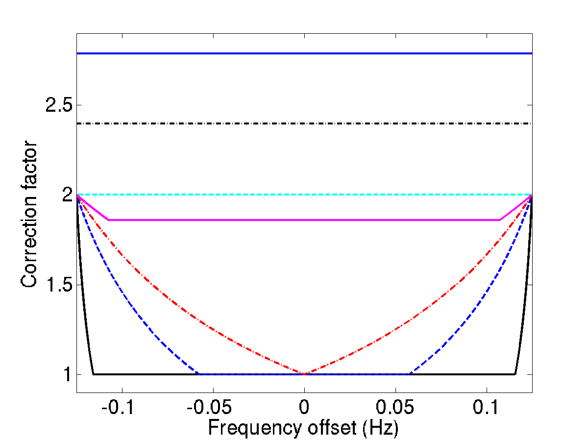
Figure 8: Simulated correction of $\hat{Y}_{\rm tot}$ for the Radiometer search across the standard 0.25 Hz-wide bin for a variety of frequencies. Bin center falls at the frequency offset of 0 Hz. The traces, from bottom to top, display the simulation for 40 (black, solid), 290 (blue, dashed), 538 (red, dot-dashed), 1000 (magenta, solid), 1076 (cyan, dashed), 1290 (black, dot-dashed), and 1500 Hz (blue, solid). Below 538 Hz note that at the bin boundary, where only half of the SNR is in this bin, the correction factor is two. The correction factor is one when the signal is completely within the bin. $\Delta f$ is larger for 290 Hz than for 40 Hz, thus the frequencies at which the injection is completely within the chosen bin (and thus has a correction factor of one) are fewer. Above 538 Hz, it is not possible to have the entire injection within a single frequency bin $df$. At most, $df/{\Delta f}$ of the injection can be within a single bin, resulting in a correction factor that is always greater than one. Above 1076 Hz, $\hat{Y}_{\rm tot}$ is always $df/{\Delta f}$ of the injection.

Above 538 Hz and at or below 1076 Hz, $df<\Delta f_{\rm obs}\leq 2*df$ and there are again three regimes to be considered: 1) when the trial injected signal is divided between the chosen frequency bin and the adjacent bin lower in frequency (while still having a maximum SNR in the chosen bin), 2) when the signal completely fills the chosen bin, and 3) when the signal is divided between the chosen frequency bin and the adjacent bin higher in frequency (while still having a maximum SNR in the chosen bin). Similar to at lower frequencies, if the injected signal falls exactly on the bin border, the recovered $\hat{Y}_{\rm tot}$ will be half the value expected from the injection and thus requires a correction factor of two. If the signal completely fills the chosen bin, the recovered $\hat{Y}_{\rm tot}$ will be the fraction of the injected signal it spans. Above 538 Hz and below 1076 Hz, Eq.’s 21 and 22 still apply to cases 1) and 3) respectively. However case 2) becomes

$$\frac{1}{C_{\rm mfb\_{trial}}}=\frac{df}{{\Delta f}}.$$ (23)

The trial correction factor as a function of frequency for the 1000 and 1076 Hz frequency bins are shown in Figure 8.

Above 1076 Hz, $\Delta f_{\rm obs}>2*df$. Here, the trial injected signal only has a maximum SNR in the chosen bin when the signal completely fills the bin. The correction factor is then always Eq. 23. The trail correction factor as a function of frequency for the 1290 and 1500 Hz bins are shown in Figure 8.

In the above discussion, the trial correction factor is exactly determined for a large number of frequencies within an individual frequency bin. In order to determine a single corrected value of $\hat{Y}_{\rm tot}$ for each frequency bin, we calculate

$$\hat{Y}_{\rm tot\_BCFcorr}=\hat{Y}_{\rm tot\_meas}\times C_{\rm mbf}$$ (24)

where $\hat{Y}_{\rm tot\_meas}$ is the (uncorrected) measured value of $\hat{Y}_{\rm tot}$ for a particular frequency bin and $C_{\rm mbf}$ is the expectation value of $C_{\rm mfb\_{trial}}$, the set of correction factors from the simulated trials. Figure 9 shows the correction factor and associated $1\sigma$ uncertainty for each frequency bin over a large range of frequency bins.

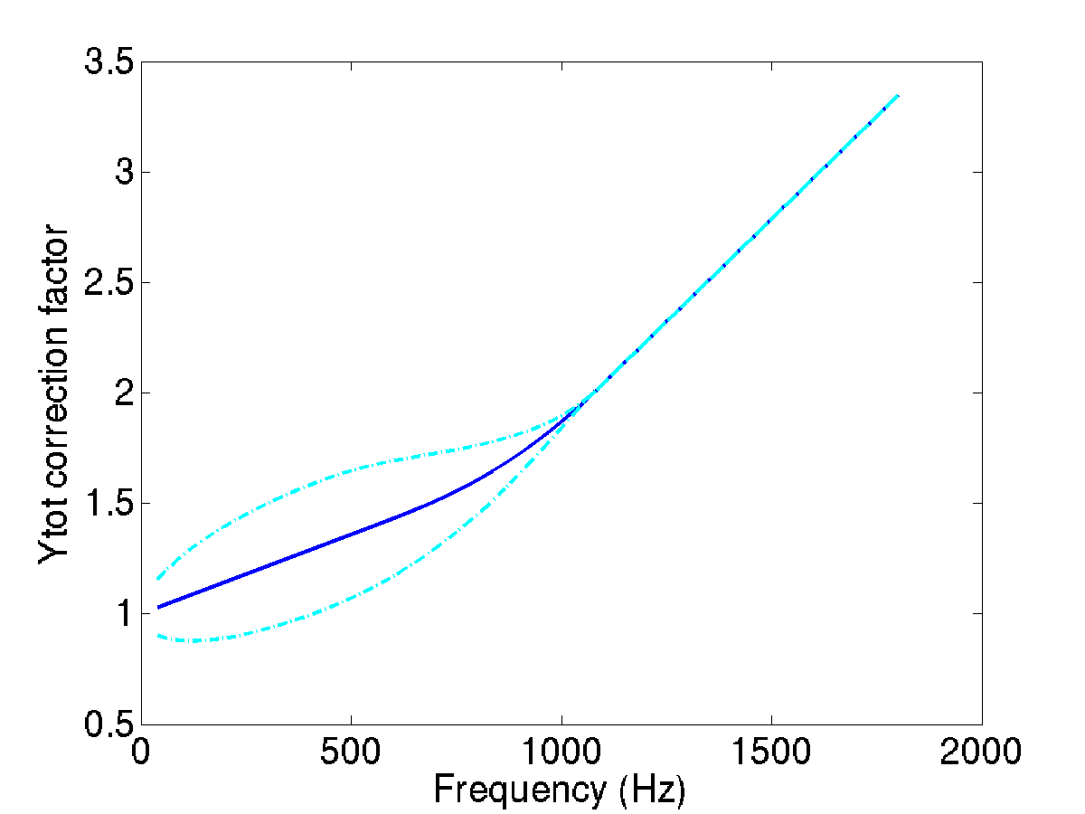
Figure 9: Frequency bin correction factor necessary to account for signals spanning multiple bins in the Radiometer search. The solid blue line denotes the correction factor and the dashed cyan lines denote its $1\sigma$ uncertainty. At low frequencies, it is statistically infrequent for a signal to span multiple frequency bins, resulting in a correction factor close to one. At high frequencies, signals always span at least two frequency bins which is reflected by the larger correction factor. The increasing uncertainty with increasing frequency below 538 Hz reflects that increasing $\Delta f$ results in fewer occurrences of a simulation falling completely within a frequency bin which results in a broadened distribution of the simulated trials. The decreasing uncertainty with increasing frequency above 538 Hz is affected by two factors. One is that increasing $\Delta f$ increases the occurrences among the simulated trials of completely spanning the frequency bin. The other factor is that the range of correction factors for a particular frequency bin lessens with increasing frequency (and hence increasing $\Delta f$).

B.5 The combined correction factor

The measured ${\hat{Y}_{\rm tot}}$, when accounting for the circular polarization assumption and for a signal spanning multiple frequency bins, is converted to $h_{0}$ by

$$h_{0}=C_{\rm cp}\times\sqrt{C_{\rm mbf}\times{\hat{Y}_{\rm tot}}df}$$ (25)

and uncertainties on this value are determined by standard propagation of error techniques for uncorrelated variables as well as the Goodman expression for exact variance Goodman (1960). Bayesian upper limits are calculated for the MDC’s 5 Hz injection search bands in which the Radiometer made no detection, using the frequency bin within the search band with the largest measured $h_{0}$ (after application of correction factors).

The conversion factors were verified with the open signals. Without correction factors applied, the average ratio of detected and measured to injected $h_{0}$ is $0.48$ and none of the 29 detected and measured $h_{0}$ agree with the injected $h_{0}$ to within one standard deviation. After applying the conversion factors, the average ratio of detected and measured to injected $h_{0}$ is $1.00$. Independent of frequency, the uncertainties were found to be too small with only 12 of the 29 detections agreeing to within one standard deviation with the injection. Work is in progress to identify the source of this discrepancy, but currently the open signals have been used to establish a factor by which to increase the error bars. Choosing a factor of $\sqrt{3}$ causes 21 of the 29 detections to agree with the injection to within one standard deviation (and all to agree within two standard deviations). The ratio of the measured and corrected to injected $h_{0}$ is shown in Figure 10.

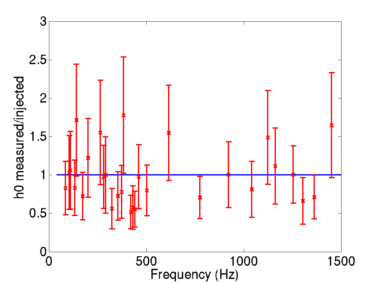
Figure 10: Ratio of measured and corrected to injected $h_{0}$ for the Radiometer search for the open signals. An extra empirical factor of $\sqrt{3}$ has been included in the uncertainties. When the measured and the injected $h_{0}$ agree to within one standard deviation, the error bars for the data (red) should intersect the blue line which has a value of one.

Appendix C TwoSpect technical details

Addition details on TwoSpect are presented in a forthcoming methods paper Meadors et al. (2015).

In this MDC, TwoSpect used Gaussian noise data from the open signal to calibrate the false alarm probability to 0.01 or better. Outliers in $R$-statistic and $p$-value were coincidence-tested; detections were required to be present in at least one interferometer pair. Initially, a threshold of $\log_{10}p=-7.75$ yielded the desired false alarm probability in bands using 840-s SFTs, but $\log_{10}p=-12.0$ was needed for 360-s SFT bands. This was found, after the deadline, to be caused by some non-Gaussian signal having been sampled in our data. If this had been known, the threshold for 360-s SFT bands could have been lower, $\log_{10}p=-8.80$, in accordance with the expectation that $p$-value thresholds should be independent of coherence time. At most one detection was lost due to this mistake.

C.1 Detection criteria

• Single-IFO candidates are the up-to-200 most extreme $p$-value outliers in a 5-Hz band that had a $\log_{10}p\leq$ threshold, where threshold = $-7.75$ if $f<$ 360.0 Hz (those that used 840-s SFTs) or $-12.0$ if $f\geq$ 360.0 Hz (those that used 360-s SFTs).

• Each candidate must survive at least one double-IFO coincidence test, involving a pairwise comparison of single-IFO candidates to see whether they are within 1/$T_{\textup{SFT}}$ in both frequency ($f$) and modulation depth ($\Delta f_{\textup{obs}}$, also known as $df$).

If there is any candidate surviving these criteria in a 5 Hz band, we mark detected, else not detected. Note that the coincidence requirement achieves the desired false alarm probability, but it means that calculating an accurate joint $p$-value for the detection would be require additional studies with computing cost beyond the scope of the MDC.

C.2 Parameter Estimation

Open signals allowed the calibration of parameter estimation methods. Signal parameters were estimated with a standard deviation according to the error in open signals, using the extremal $p$-value for a coincident signal to read the estimated parameters. In addition to the uncertainty inherent in this procedure, there is also a systematic uncertainty due to $\cos\iota$, because the pipeline is instead sensitive to the circularly-polarized-equivalent, $h_{0}^{\text{eff}}$, defined in (19) This systematic error is also included in the uncertainties for $h_{0}$.

Upper limits and detection efficiency estimates were made using open pulsar data.

C.3 Ambiguity between $h_{0}$ and $\cos\iota$

The cosine of the inclination angle of the pulsar, $\cos\iota$, casts an ambiguity over the determination of $h_{0}$. For TwoSpect, which assumes circular polarization, the approximate true value of $h_{0}$ will indeed be as reported if $|\cos\iota|$ = 1, but will be greater for smaller $|\cos\iota|$ is less (i.e., the GW is elliptically polarized). In the case of linear polarization, $h_{0}$ will be about $2^{3/2}\approx 2.83$ times larger than reported. A simulation of $2\times 10^{6}$ pulsars, generated uniformly in $1/h_{0}$ for $h_{0}$ between $3\times 10^{-26}$ and $3\times 10^{-24}$, demonstrated that the average factor is 1.74 with $1\sigma$-uncertainty of $\pm 0.37$.

We validated the fraction of open analyses that estimated $h_{0}$, $f$ and $a\sin i$ within their 1-$\sigma$ error bars:

• $h_{0}$: 77.4%

• $f$: 74.2%

• $asini$: 67.7%

• Period: 100% with only 68023.8259 s tried

Because these percentages are larger than fraction expected in 1-$\sigma$, the parameter estimation uncertainties for the open data set were conservative.

Appendix D CrossCorr technical details

Complete details of the CrossCorr analysis as implemented for the MDC will appear in Zhang et al. (2015). This appendix briefly describes the most important aspects.

D.1 Choice of $T_{\text{max}}$ parameter

Table 12: Choice of SFT durations and coherence times for the cross-correlation search.

Freq range	$T_{\text{sft}}$(s)	$T_{\text{max,inner}}$(s)	$T_{\text{max,outer}}$ (s)
$50$–$100$	$900$	$5400$	$3600$
$100$–$200$	$600$	$2400$	$1200$
$200$–$400$	$420$	$2100$	$840$
$400$–$800$	$300$	$1140$	$840$
$800$–$1375$	$240$	$780$	$540$

As described in Sec. D.1, the cross-correlation search used a different duration $T_{\text{sft}}$ for the Fourier transforms of the data as a function of frequency. It also used two different values of maximum allowed time offset $T_{\text{max}}$ between correlated SFTs for the two regions of parameter space shown in Fig. 11. These choices were made to balance computing cost and sensitivity.

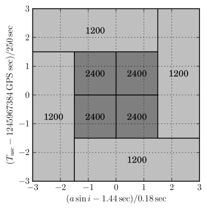
Figure 11: Example of $T_{\text{max}}$ values for the CrossCorr search divided according to orbital parameter space. The “inner regions”, which are more likely to contain the signal parameters, use a longer coherence length $T_{\text{max}}$.

The primary determining factor in both the sensitivity and computational cost of the CrossCorr search is the coherence time $T_{\text{max}}$. This is the maximum time offset allowed between pairs of SFTs to be included in the CrossCorr statistic. Use of a single $T_{\text{max}}$ value for the entire MDC would not have been ideal for two reasons:

• The density of templates in each of the orbital parameter space directions ($a\sin i$ and $T_{\text{asc}}$) grows with frequency. Additionally, since the method treats the Doppler-shifted frequency as constant over an SFT, the SFT length needs to be decreased with frequency in order to avoid loss of SNR due to unmodelled Doppler acceleration. These two effects mean a search with the same $T_{\text{max}}$ will be more computationally expensive at higher frequencies.

• If the prior uncertainties on orbital parameters are assumed to be Gaussian distributed (as they were for the MDC), the “inner” regions of parameter space (close to the most likely values) are more likely to contain the signal parameters than the “outer” regions.

Since it is impractical to have the coherence time $T_{\text{max}}$ (and the SFT duration $T_{\text{sft}}$) vary continuously with frequency, the CrossCorr search was implemented with a single setup for all of the frequency bands lying in a particular “octave”, as described in Table 12. The setups were chosen to have roughly constant computing cost (estimated as proportional to the number of parameter space templates times the number of SFT pairs) for each 5 Hz band. To determine the ideal coherence time $T_{\text{sft}}$ within this constraint, the orbital parameter space was divided into “inner” and “outer” regions, as shown in Figure 11. The “inner” regions, with both $a\sin i$ and $T_{\text{asc}}$ within 1.5 standard deviations ($1.5\sigma$) of their a priori most likely values, had, according to the assumed Gaussian prior distribution, a $75.1\%$ probability of containing any given signal. The outer regions, where both parameters were within $3\sigma$ of their most likely value, but at least one was more than $1.5\sigma$ away, constituted three times the area in parameter space, but only had a $24.4\%$ chance of containing the signal. Different combinations of $T_{\text{max,inner}}$ and $T_{\text{max,outer}}$ which fit within the computing budget were considered, and the ones which provided the greatest overall likelihood of producing a detection (considering the probability of the signal lying in each region and the conditional probability of observing a high enough statistic value with the chosen $T_{\text{max}}$, if the signal was in that region) were chosen. These are summarized in Table 12.

D.2 Detection confidence

A naïve estimate of significance for the CrossCorr search, which constructs a statistic which in the absence of a signal has zero mean and unit variance, is to assume the distribution to be Gaussian. The single-template false-alarm probability corresponding to a value $\rho$ for the statistic defined in (11) is then

$$p_{1}=\frac{1}{2}\operatorname{erfc}\left(\frac{\rho}{\sqrt{2}}\right)\approx\frac{e^{-\rho^{2}/2}}{\rho\sqrt{2\pi}}(1-\rho^{-2})$$ (26)

where the asymptotic form of the complementary error function should be used to avoid underflow when $\rho>20$. To estimate a combined $p$-value of a search using $N$ templates, these were assumed to be $N$ independent trials and constructs the per-band false alarm probability corresponding to the maximum $\rho$ over the band:

$$p_{N}=1-(1-p_{1})^{N}\approx 1-e^{Np_{1}}\approx Np_{1}$$ (27)

where the first approximation is valid when $N$ is large and $p_{1}$ is small, and the second is valid when $Np_{1}$ is also small. The nominal detection threshold would be $p_{N}<10^{-2}$, however with $N\sim 10^{8}$ templates per band, the Gaussian approximation (26) will be invalid at the required small values of $p_{1}\lesssim 10^{-10}$. Since the methods described in Whelan et al. (2015) for estimating the false-alarm probability more accurately were not implemented at the time of the analysis, the naïve value $p_{N}$ was calculated. Although the resulting values do not represent a realistic quantification of the false-alarm probability (and are therefore not shown in Figure2), they can be compared to the results of 49 searches over signal-free bands similar to the closed signal bands of the MDC. The lowest naïve $p$-value from those searches, which wa s $p_{N}=7.5\times 10^{-5}$, provides an empirical estimate of an actual $p$-value of $1.02\%$. In comparison, the highest naïve $p$-value for any closed signal was $p_{N}=3.4\times 10^{-129}$, so it is possible to comfortably declare all of them to be confident detections, even without reliable $p$-values.

D.3 Parameter estimation and errorbars

The CrossCorr search is performed over a grid of templates in $f$, $a\sin i$ and $T_{\text{asc}}$, whose spacing is determined by the metric given in Whelan et al. (2015). The spacing in each direction scales (in cases where $T_{\text{max}}$ is small compared to the orbital period, as it was for the MDC analysis) as $\sqrt{m}/T_{\text{max}}$, where $m$ is the chosen mismatch and $T_{\text{max}}$ is the maximum time separation allowed between pairs of SFTs to be included in the cross-correlation. Additionally, the spacing in $a\sin i$ and $T_{\text{asc}}$ each scale as $1/f_{0}$ and the spacing in $T_{\text{asc}}$ scales as $1/(a\sin i)$. The initial grid spacing was chosen to produce a mismatch of around $0.25$. A refined grid of $13\times 13\times 13$ points, with one-third the original spacing, was then generated around the loudest candidate signal in the band. For some quieter signals there was a further followup with a larger value of $T_{\text{max}}$ to produce an even finer $13\times 13\times 13$ grid centered on the loudest candidate in the refined grid. For parameter estimation purposes, an interpolation procedure was used, where the statistic values in a $3\times 3\times 3$ subgrid of the final fine grid, centered on the loudest value, were fit to a multivariate quadratic. The peak of this quadratic function was chosen as the best estimate of the parameters, allowing them to be estimated more accurately than the spacing of the final grid. The errorbars quoted for the CrossCorr results are a quadrature combination of three effects: the usual statistical uncertainty associated with the unknown noise realization (which scales inversely with the observed $\rho$ value), an interpolation error estimated using the residuals of the quadratic fit, and a systematic uncertainty associated with the unknown value of $\cos\iota$. Parameter estimates were produced using this method for the open signals and compared to the actual parameter values. The actual offsets between estimated and true parameters were mostly consistent with the estimated uncertainties, aside from two observed effects described in the following sections. Analysis of this effects led to an empirically-determined modifications to the procedure, and this modified procedure was used to obtain the parameter estimates and errorbars for the closed data.

D.3.1 Empirical adjustment of $a\sin i$ values

Analysis of the open signals indicated that the $a\sin i$ estimates were systematically lower than the true values, with the qualitative feature that the underestimates were larger at lower frequencies. The explanation for this is unknown, but the dependence was assumed on dimensional grounds to be inversely proportional to frequency. The proportionally constant was estimated from the open signals, and the adjustment was made to replace the old estimate with

$$(a\sin i)_{\text{est,new}}=(a\sin i)_{\text{est,old}}+\frac{0.028}{f_{0}}$$ (28)

In order to produce conservative estimates of our parameter uncertainties, this offset amount $0.028/f_{0}$ was combined in quadrature with the other three contributions to the errorbars reported for $a\sin i$.

D.3.2 Empirical adjustment of statistical errorbars for loud signals

A second discrepancy seen in the recovered parameters of the open signals was that some of the loudest recovered signals ($\rho\gtrsim 300$) had recovered parameters (especially $T_{\text{asc}}$) which were significantly larger than the calculated erorrbars would suggest. A conjectured explanation is that the expressions used for generating the statistical errorbars neglected higher order terms in the signal amplitude $h_{0}$. Scaling arguments indicate that the relative size of such terms should be $\sim\rho/\sqrt{N_{\text{pairs}}}$. The statistical errorbars for all parameters were thus increased by a factor of $1+150\frac{\rho}{\sqrt{N_{\text{pairs}}}}$, where the coefficient $150$ was empirically determined to make the $T_{\text{asc}}$ errorbars calculated from the open data consistent with the actual parameter offsets.

References

- Aasi et al. (2015) J. Aasi et al. (LIGO Scientific Collaboration), “Advanced LIGO,” Class. Quant. Grav. 32, 074001 (2015), arXiv:1411.4547 .
- Acernese et al. (2015a) F. Acernese et al. (Virgo Collaboration), “Advanced Virgo: a second-generation interferometric gravitational wave detector,” Class. Quant. Grav. 32, 024001 (2015a), arXiv:1408.3978 .
- Papaloizou and Pringle (1978) J. Papaloizou and J. E. Pringle, “Gravitational radiation and the stability of rotating stars,” Mon. Not. R. Astron. Soc. 184, 501–508 (1978).
- Wagoner (1984) R. V. Wagoner, “Gravitational radiation from accreting neutron stars,” Astrophys. J. 278, 345–348 (1984).
- Bildsten (1998) L. Bildsten, “Gravitational Radiation and Rotation of Accreting Neutron Stars,” Astrophys. J. Lett. 501, L89–L93 (1998), astro-ph/9804325 .
- Ushomirsky et al. (2000) G. Ushomirsky, C. Cutler, and L. Bildsten, “Deformations of accreting neutron star crusts and gravitational wave emission,” Mon. Not. R. Astron. Soc. 319, 902–932 (2000), astro-ph/0001136 .
- Cutler (2002) C. Cutler, “Gravitational waves from neutron stars with large toroidal B fields,” Phys. Rev. D 66, 084025 (2002), gr-qc/0206051 .
- Premachandra (2015) S. Premachandra, Precision ephemerides of neutron star binaries to assist gravitational wave searches: Sco X-1 & Cyg X-2, Ph.D. thesis, Monash (2015).
- Abbott et al. (2007a) B. Abbott et al. (LIGO Scientific Collaboration), “Upper limit map of a background of gravitational waves,” Phys. Rev. D 76, 082003 (2007a), astro-ph/0703234 .
- Abbott et al. (2007b) B. Abbott et al. (LIGO Scientific Collaboration), “Searches for periodic gravitational waves from unknown isolated sources and Scorpius X-1: Results from the second LIGO science run,” Phys. Rev. D 76, 082001 (2007b), gr-qc/0605028 .
- Abbott et al. (2011) B. P. Abbott et al. (LIGO Scientific Collaboration and Virgo Collaboration), “Directional limits on persistent gravitational waves using ligo s5 science data,” Phys. Rev. Lett. 107, 271102 (2011), arXiv:1109.1809 .
- Aasi et al. (2014a) J. Aasi et al. (LIGO Scientific Collaboration and Virgo Collaboration), “First all-sky search for continuous gravitational waves from unknown sources in binary systems,” Phys. Rev. D 90, 062010 (2014a).
- Aasi et al. (2014b) J. Aasi et al. (LIGO Scientific Collaboration and Virgo Collaboration), “A directed search for gravitational waves from Scorpius X-1 with initial LIGO,” (2014b), arXiv:1412.0605 .
- The LIGO Scientific Collaboration et al. (2015) The LIGO Scientific Collaboration, J. Aasi, B. P. Abbott, . Abbott, T. Abbott, M. R. Abernathy, K. Ackley, C. Adams, T. Adams, P. Addesso, and et al., “Advanced LIGO,” Classical and Quantum Gravity 32, 074001 (2015), arXiv:1411.4547 [gr-qc] .
- LIGO Scientific Collaboration et al. (2013) LIGO Scientific Collaboration, Virgo Collaboration, J. Aasi, J. Abadie, B. P. Abbott, R. Abbott, T. D. Abbott, M. Abernathy, T. Accadia, F. Acernese, and et al., “Prospects for Localization of Gravitational Wave Transients by the Advanced LIGO and Advanced Virgo Observatories,” ArXiv e-prints (2013), arXiv:1304.0670 [gr-qc] .
- Harry (2010) Gregory M. Harry (LIGO Scientific), “Advanced LIGO: The next generation of gravitational wave detectors,” Class.Quant.Grav. 27, 084006 (2010).
- Acernese et al. (2015b) F. Acernese et al. (VIRGO), “Advanced Virgo: a second-generation interferometric gravitational wave detector,” Class.Quant.Grav. 32, 024001 (2015b), arXiv:1408.3978 [gr-qc] .
- Roy et al. (2015) J. Roy et al., “Discovery of Psr J1227-4853: A Transition from a Low-mass X-Ray Binary to a Redback Millisecond Pulsar,” Astrophys. J. Lett. 800, L12 (2015), arXiv:1412.4735 .
- Deller et al. (2014) A. T. Deller et al., “Radio imaging observations of PSR J1023+0038 in an LMXB state,” (2014), arXiv:1412.5155 .
- Tendulkar et al. (2014) S. P. Tendulkar et al., “NuSTAR Observations of the State Transition of Millisecond Pulsar Binary PSR J1023+0038,” Astrophys. J. 791, 77 (2014), arXiv:1406.7009 .
- Bogdanov et al. (2014) S. Bogdanov et al., “Coordinated X-ray, Ultraviolet, Optical, and Radio Observations of the PSR J1023+0038 System in a Low-mass X-ray Binary State,” (2014), arXiv:1412.5145 .
- Steeghs and Casares (2002) D. Steeghs and J. Casares, “The Mass Donor of Scorpius X-1 Revealed,” Astrophys. J. 568, 273–278 (2002), arXiv:astro-ph/0107343 .
- Galloway et al. (2014) D. K. Galloway, S. Premachandra, D. Steeghs, T. Marsh, J. Casares, and R. Cornelisse, “Precision Ephemerides for Gravitational-wave Searches. I. Sco X-1,” Astrophys. J. 781, 14 (2014), arXiv:1311.6246 .
- Watts et al. (2008) A. L. Watts, B. Krishnan, L. Bildsten, and B. F. Schutz, “Detecting gravitational wave emission from the known accreting neutron stars,” Mon. Not. R. Astron. Soc. 389, 839–868 (2008), arXiv:0803.4097 .
- Haskell et al. (2015) B. Haskell, M. Priymak, A. Patruno, M. Oppenoorth, A. Melatos, and P. Lasky, “Detecting gravitational waves from mountains on neutron stars in the Advanced Detector Era,” (2015), arXiv:1501.06039 .
- Bradshaw et al. (1999) C. F. Bradshaw, E. B. Fomalont, and B. J. Geldzahler, Astrophys. J. Lett. 512, L121 (1999).
- Liu et al. (2007) Q. Z. Liu, J. van Paradijs, and E. P. J. van den Heuvel, “A catalogue of low-mass X-ray binaries in the Galaxy, LMC, and SMC (Fourth edition),” Astron. Astrophys. 469, 807–810 (2007), arXiv:0707.0544 .
- Leaci and Prix (2015) Paola Leaci and Reinhard Prix, “Directed searches for continuous gravitational waves from binary systems: parameter-space metrics and optimal Scorpius X-1 sensitivity,” (2015), arXiv:1502.00914 .
- Middleditch and Priedhorsky (1986) J. Middleditch and W. C. Priedhorsky, “Discovery of rapid quasi-periodic oscillations in Scorpius X-1,” Astrophys. J. 306, 230–237 (1986).
- Wood et al. (1991) K. S. Wood et al., “Searches for millisecond pulsations in low-mass X-ray binaries,” Astrophys. J. 379, 295–309 (1991).
- Hertz et al. (1992) P. Hertz et al., “X-ray variability of Scorpius X-1 during a multiwavelength campaign,” Astrophys. J. 396, 201–218 (1992).
- Vaughan et al. (1994) B. A. Vaughan et al., “Searches for millisecond pulsations in low-mass X-ray binaries, 2,” Astrophys. J. 435, 362–371 (1994).
- Jahoda et al. (1996) K. Jahoda et al., “In-orbit performance and calibration of the Rossi X-ray Timing Explorer (RXTE) Proportional Counter Array (PCA),” Proc. SPIE 2808, 59–70 (1996).
- van der Klis et al. (1996) M. van der Klis et al., “Discovery of Submillisecond Quasi-periodic Oscillations in the X-Ray Flux of Scorpius X-1,” Astrophys. J. Lett. 469, L1 (1996), astro-ph/9607047 .
- van der Klis et al. (1997) M. van der Klis, R. A. D. Wijnands, K. Horne, and W. Chen, “Kilohertz Quasi-Periodic Oscillation Peak Separation Is Not Constant in Scorpius X-1,” Astrophys. J. Lett. 481, L97–L100 (1997), astro-ph/9703025 .
- Méndez and van der Klis (2000) M. Méndez and M. van der Klis, “The harmonic and sideband structure of the kilohertz quasi-periodic oscillations in Sco X-1,” Mon. Not. R. Astron. Soc. 318, 938–942 (2000), astro-ph/0006243 .
- Skrutskie et al. (2006) M. F. Skrutskie et al., “The Two Micron All Sky Survey (2MASS),” The Astronomical Journal 131, 1163–1183 (2006).
- Fomalont et al. (2001) E. B. Fomalont, B. J. Geldzahler, and C. F. Bradshaw, “Scorpius X-1: The Evolution and Nature of the Twin Compact Radio Lobes,” Astrophys. J. 558, 283–301 (2001), astro-ph/0104372 .
- Bildsten et al. (1997) L. Bildsten et al., “Observations of Accreting Pulsars,” Astrophys. J. Supp. 113, 367–408 (1997), astro-ph/9707125 .
- Baykal and Oegelman (1993) A. Baykal and H. Oegelman, “An empirical torque noise and spin-up model for accretion-powered X-ray pulsars,” Astron. Astrophys. 267, 119–125 (1993).
- King (2006) A. R. King, “Accretion in compact binaries,” in Compact stellar X-ray sources, edited by W. H. G. Lewin and M. van der Klis (2006) pp. 507–546.
- van der Putten et al. (2010) S. van der Putten, H. J. Bulten, J. F. J. van den Brand, and M. Holtrop, “Searching for gravitational waves from pulsars in binary systems: An all-sky search,” J. Phys. Conf. Ser. 228, 012005 (2010).
- Bonferroni (1935) C. E. Bonferroni, “Il calcolo delle assicurazioni su gruppi di teste,” Studi in Onore del Professore Salvatore Ortu Carboni, , 13–60 (1935).
- Bonferroni (1936) C. E. Bonferroni, “Teoria statistica delle classi e calcolo delle probabilità,” Pubblicazioni del R Istituto Superiore di Scienze Economiche e Commerciali di Firenze 8, 3–62 (1936).
- Ballmer (2006) Stefan W. Ballmer, “A radiometer for stochastic gravitational waves,” Class. Quant. Grav. 23, S179–S186 (2006), gr-qc/0510096 .
- Messenger and Woan (2007) C. Messenger and G. Woan, “A Fast search strategy for gravitational waves from low-mass X-ray binaries,” Class. Quant. Grav. 24, S469–S480 (2007), arXiv:gr-qc/0703155 .
- Sammut et al. (2014) L. Sammut, C. Messenger, A. Melatos, and B. J. Owen, “Implementation of the frequency-modulated sideband search method for gravitational waves from low mass x-ray binaries,” Phys. Rev. D 89, 043001 (2014), arXiv:1311.1379 .
- Ransom et al. (2003) S. M. Ransom, J. M. Cordes, and S. S. Eikenberry, “A New Search Technique for Short Orbital Period Binary Pulsars,” Astrophys. J. 589, 911–920 (2003), astro-ph/0210010 .
- Jaranowski et al. (1998) Piotr Jaranowski, Andrzej Krolak, and Bernard F. Schutz, “Data analysis of gravitational-wave signals from spinning neutron stars. I: The signal and its detection,” Phys. Rev. D 58, 063001 (1998), arXiv:gr-qc/9804014 .
- Goetz and Riles (2011) E. Goetz and K. Riles, “An all-sky search algorithm for continuous gravitational waves from spinning neutron stars in binary systems,” Classical and Quantum Gravity 28, 215006 (2011), arXiv:1103.1301 .
- Dhurandhar et al. (2008) Sanjeev Dhurandhar, Badri Krishnan, Himan Mukhopadhyay, and John T. Whelan, “The cross-correlation search for periodic gravitational waves,” Phys. Rev. D 77, 082001 (2008), arXiv:0712.1578 .
- Chung et al. (2011) Christine Chung, Andrew Melatos, Badri Krishnan, and John T. Whelan, “Designing a cross-correlation search for continuous-wave gravitational radiation from a neutron star in the supernova remnant SNR 1987A,” Mon. Not. R. Astron. Soc. 414, 2650–2663 (2011), arXiv:1102.4654 .
- Whelan et al. (2015) John T. Whelan, Santosh Sundaresan, Yuanhao Zhang, and Prabath Peiris, “A Model-Based Cross-Correlation Search for Gravitational Waves from Scorpius X-1,” LIGO DCC P1200142 (2015).
- (54) Einstein@Home website, http://einstein.phys.uwm.edu/.
- Aasi et al. (2013) J. Aasi et al. (LIGO Scientific Collaboration and Virgo Collaboration), “Einstein@Home all-sky search for periodic gravitational waves in LIGO S5 data,” Phys. Rev. D 87, 042001 (2013), arXiv:1207.7176 .
- Knispel et al. (2011) B. Knispel et al., “Arecibo PALFA Survey and Einstein@Home: Binary Pulsar Discovery by Volunteer Computing,” Astrophys. J. 732, L1 (2011), arXiv:1102.5340 .
- Knispel et al. (2013) B. Knispel et al., “Einstein@Home Discovery of 24 Pulsars in the Parkes Multi-beam Pulsar Survey,” Astrophys. J. 774, 93 (2013), arXiv:1302.0467 .
- Allen et al. (2013) B. Allen et al., “The Einstein@Home search for radio pulsars and PSR J2007+2722 discovery,” Astrophys. J. 773, 91 (2013), arXiv:1303.0028 .
- Pletsch et al. (2013) H. J. Pletsch et al., “Einstein@Home discovery of four young gamma-ray pulsars in LAT data,” Astrophys. J. 779, L11 (2013), arXiv:1311.6427 .
- Prix (2007) Reinhard Prix, “Search for continuous gravitational waves: Metric of the multi-detector F-statistic,” Phys. Rev. D 75, 023004 (2007), arXiv:gr-qc/0606088 .
- Brady and Creighton (2000) Patrick R. Brady and Teviet Creighton, “Searching for periodic sources with LIGO. 2. Hierarchical searches,” Phys. Rev. D 61, 082001 (2000), arXiv:gr-qc/9812014 .
- Wette (2012) Karl Wette, “Estimating the sensitivity of wide-parameter-space searches for gravitational-wave pulsars,” Phys. Rev. D 85, 042003 (2012), arXiv:1111.5650 .
- Prix and Shaltev (2012) Reinhard Prix and Miroslav Shaltev, “Search for Continuous Gravitational Waves: Optimal StackSlide method at fixed computing cost,” Phys. Rev. D 85, 084010 (2012), arXiv:1201.4321 .
- Meadors et al. (2015) G.D. Meadors, E. Goetz, and K. Riles, “Twospect: search for a simulated scorpius x-1,” LIGO DCC P1500037 (2015).
- (65) “LSC Algorithm Library Suite,” https://www.lsc-group.phys.uwm.edu/daswg/projects/lalsuite.html.
- D. Buskulic et al. (2014) D. Buskulic, I. Fiori, F. Marion, and B. Mours, “The frame vector library (frv),” http://lappweb.in2p3.fr/virgo/FrameL/ (2014).
- Zhang et al. (2015) Yuanhao Zhang, John T. Whelan, and Badri Krishnan, “Results of a Model-Based Cross-Correlation Search for Signals from Scorpius X-1 in Mock Gravitational-Wave Data,” LIGO DCC P1400216 (2015).
- Prix (2011) Reinhard Prix, “The -statistic and its implementation in ComputeFstatistic_v2,” LIGO Technical Document LIGO-T0900149-v5 (2011).
- Goodman (1960) L.A. Goodman, “On the exact variance of products,” Journal of the American Statistical Association 55, 708–713 (1960).