In this paper, we introduce a new analogue of Bernstein-Kantorovich operators which we call as $(p,q)$-Bernstein-Kantorovich operators. We discuss approximation properties for these operators based on Korovkin’s type approximation theorem and we compute the order of convergence using usual modulus of continuity and also the rate of convergence when the function $f$ belongs to the class Lip${}_{M}(\alpha)$. Moreover, we also study the local approximation property of the sequence of positive linear operators $K_{n}^{(p,q)}$. We show comparisons and some illustrative graphics for the convergence of operators to a function. In comparison to $q$-analogoue of Bernstein-Kantorovich operators, our generalization gives more flexibility for the convergence of operators to a function.

Keywords and phrases: $(p,q)$-integers; $(p,q)$-Bernstein-Kantorovich operators; $q$-Bernstein-Kantorovich operators; modulus of continuity; positive linear operators; Korovkin type approximation theorem.

AMS Subject Classifications (2010): 41A10, 41A25, 41A36

1 Introduction and preliminaries

During the last two decades, the applications of $q$-calculus emerged as a new area in the field of approximation theory. The rapid development of $q$-calculus has led to the discovery of various generalizations of Bernstein polynomials involving $q$-integers. The aim of these generalizations is to provide appropriate and powerful tools to application areas such as numerical analysis, computer-aided geometric design and solutions of differential equations.

Using $q$-integers, Lupaş [15] introduced the first $q$-Bernstein operators [4] and investigated its approximating and shape-preserving properties. Another $q$-analogue of the Bernstein polynomials is due to Phillips [26]. Since then several generalizations of well-known positive linear operators based on $q$-integers have been introduced and studied their approximation properties. For instance, $q$-Bleimann, Butzer and Hahn operators [3]; $q$-parametric Szász-Mirakjan operators [16]; $q$-Bernstein-Durrmeyer operators [17]; $q$-analogue of Szász-Kantorovich operators [18].

Recently, Mursaleen et al introduced $(p,q)$-calculus in approximation theory and constructed the $(p,q)$-analogue of Bernstein operators [21] and $(p,q)$-analogue of Bernstein-Stancu operators [23], $(p,q)$-analogue of Bleimann-Butzer-Hahm operators [24], Bernstein-Schurer operarors [25] and investigated their approximation properties. The $(p,q)$-analog of Szász-Mirakyan operators [1], Kantorovich type Bernstein-Stancu-Schurer operators [5] and Kantorovich variant of $(p,q)$-Szász-Mirakjan operators [19] have recently been studied too.

Motivated by their work, in this article, authors introduce a new analogue of Bernstein-Kantorovich operators. Paper is organized as follows: In Section 2, we define $(p,q)$-Bernstein-Kantorovich operators and establish a bsic lemma which is used in proving main results. In Section 3, we discuss approximation properties for these operators based on Korovkin’s type approximation theorem and we compute the order of convergence using usual modulus of continuity and also the rate of convergence when the function $f$ belongs to the class Lip${}_{M}(\alpha)$. Moreover, we also study the local approximation property of the sequence of positive linear operators $K_{n}^{(p,q)}$. In Section 4, we give some examples to show comparisons and some illustrative graphics for the convergence of operators to a function.

Let us recall certain definitions and notations of $(p,q)$-calculus:

The $(p,q)$-integer was introduced in order to generalize or unify several forms of $q$-oscillator algebras well known in the earlier physics literature related to the representation theory of single parameter quantum algebras [6]. The $(p,q)$-integer $[n]_{p,q}$ is defined by

$$[n]_{p,q}:=\frac{p^{n}-q^{n}}{p-q},~{}~{}~{}n=0,1,2,\cdots,~{}~{}0<q<p\leq 1.$$

$$\left[k\right]_{p,q}!:=\left\{\begin{array}[]{lll}\left[k\right]_{p,q}\left[k-1\right]_{p,q}...1&,&k\geq 1,\\ 1,&&k=0\end{array}\right.$$

The $(p,q)$-Binomial expansion is

$$(x+y)_{p,q}^{n}:=(x+y)(px+qy)(p^{2}x+q^{2}y)\cdots(p^{n-1}x+q^{n-1}y)$$

and the $(p,q)$-binomial coefficients are defined by

$$\left[\begin{array}[]{c}n\\ k\end{array}\right]_{p,q}:=\frac{[n]_{p,q}!}{[k]_{p,q}![n-k]_{p,q}!}.$$

The definite integrals of the function $f$ are defined by

$$\int_{0}^{a}f(x)d_{p,q}x=(q-p)a\sum\limits_{k=0}^{\infty}\frac{p^{k}}{q^{k+1}}f\left(\frac{p^{k}}{q^{k+1}}a\right),~{}~{}~{}\text{when}~{}~{}~{}\left|\frac{p}{q}\right|<1,$$

and

$$\int_{0}^{a}f(x)d_{p,q}x=(p-q)a\sum\limits_{k=0}^{\infty}\frac{q^{k}}{p^{k+1}}f\left(\frac{q^{k}}{p^{k+1}}a\right),~{}~{}~{}\text{when}~{}~{}~{}\left|\frac{p}{q}\right|>1.$$

Details on $(p,q)$-calculus can be found in [9, 13, 14, 27, 28]. For $p=1$, all the notions of $(p,q)$-calculus are reduced to $q$-calculus [10].

2 Construction of Operators

Mursaleen et. al [21] introduced $(p,q)$-analogue of Bernstein operators as

$$B_{n,p,q}(f;x)=\sum\limits_{k=0}^{n}\left[\begin{array}[]{c}n\\ k\end{array}\right]_{p,q}x^{k}\prod\limits_{s=0}^{n-k-1}(p^{s}-q^{s}x)~{}~{}f\left(\frac{[k]_{p,q}}{[n]_{p,q}}\right),~{}~{}x\in[0,1].$$

But $B_{n,p,q}(1;x)\neq 1$ for all $x\in[0,1]$. Hence, they re-introduced their operators in [22] as follows :

$$B_{n,p,q}(f;x)=\frac{1}{p^{\frac{n(n-1)}{2}}}\sum\limits_{k=0}^{n}\left[\begin{array}[]{c}n\\ k\end{array}\right]_{p,q}p^{\frac{k(k-1)}{2}}x^{k}\prod\limits_{s=0}^{n-k-1}(p^{s}-q^{s}x)~{}~{}f\left(\frac{[k]_{p,q}}{p^{k-n}[n]_{p,q}}\right),~{}~{}x\in[0,1].$$

The same problem was occurring with the operators introduced in [23]. So the revised form of $(p,q)$-analogue of Bernstein-Stancu operators are given as follows:

$$S_{n,p,q}(f;x)=\frac{1}{p^{\frac{n(n-1)}{2}}}\sum\limits_{k=0}^{n}\left[\begin{array}[]{c}n\\ k\end{array}\right]_{p,q}p^{\frac{k(k-1)}{2}}x^{k}\prod\limits_{s=0}^{n-k-1}(p^{s}-q^{s}x)~{}~{}f\left(\frac{{p^{n-k}[k]_{p,q}+\alpha}}{[n]_{p,q}+\beta}\right),~{}~{}x\in[0,1].$$

Note that for $p=1$, $(p,q)$-Bernstein operators and $(p,q)$-Bernstein-Stancu operators turn out to be $q$-Bernstein operators and $q$-Bernstein-Stancu operators, respectively.

Dalmanoglu [7] defined the Bernstein-Kantorovich [11] operators using $q$-calculus as follows:

$$K_{n,q}(f;x)=[n+1]_{q}\sum\limits_{k=0}^{n}p_{n,k}(q;x)\int_{{[k]_{q}}/{[n+1]_{q}}}^{{[k+1]_{q}}/{[n+1]_{q}}}f(t)d_{q}t,~{}~{}x\in[0,1],$$

$$p_{n,k}(q;x):=\left[\begin{array}[]{c}n\\ k\end{array}\right]_{q}x^{k}\prod\limits_{s=0}^{n-k-1}(1-q^{s}x).$$

where $K_{n,q}:$ $C[0,1]\rightarrow C[0,1]$ are defined for any $n\in\mathbb{N}$ and for any function $f\in C[0,1].$

Now, we introduce $(p,q)$-analogue of Bernstein-Kantorovich operators as

$$K_{n}^{(p,q)}(f;x)=\frac{[n]_{p,q}}{p^{\frac{n(n-1)}{2}}}\sum\limits_{k=0}^{n}\frac{b_{n,k}^{(p,q)}(x)}{p^{n-k}q^{k}}\int_{\frac{[k]_{p,q}}{p^{k-n-1}~{}[n]_{p,q}}}^{\frac{[k+1]_{p,q}}{p^{k-n}~{}[n]_{p,q}}}f(t)d_{p,q}t,~{}~{}x\in[0,1]$$

where

$$b_{n,k}^{(p,q)}(x)=\left[\begin{array}[]{c}n\\ k\end{array}\right]_{p,q}~{}(x)_{p,q}^{k}(1-x)_{p,q}^{n-k}=\left[\begin{array}[]{c}n\\ k\end{array}\right]_{p,q}~{}p^{\frac{k(k-1)}{2}}x^{k}(1-x)_{p,q}^{n-k}=\left[\begin{array}[]{c}n\\ k\end{array}\right]_{p,q}p^{\frac{k(k-1)}{2}}x^{k}\prod\limits_{s=0}^{n-k-1}(p^{s}-q^{s}x)$$

and $(x)_{p,q}^{k}:=x(px)(p^{2}x)\cdots(p^{k-1}x)=p^{\frac{k(k-1)}{2}}x^{k}$, and $f$ is a non-decreasing function.

For $p=1$, operators (2.1) turns out to be the classical $q$-Bernstein-Kantorovich operators.

First, we prove the following basic lemmas:

Lemma 2.1. For $x\in[0,1],~{}0<q<p\leq 1$

• $K_{n}^{(p,q)}(1;x)=1$,

• $K_{n}^{(p,q)}(t;x)=x+\frac{p^{n}}{[2]_{p,q}[n]_{p,q}}$,

• $K_{n}^{(p,q)}(t^{2};x)=\frac{q}{p}\frac{[n-1]_{p,q}}{[n]_{p,q}}x^{2}+\Big{(}\frac{p^{n}(2q+p)}{[3]_{p,q}[n]_{p,q}}+\frac{p^{n-1}}{[n]_{p,q}}\Big{)}x+\frac{p^{2n}}{[3]_{p,q}[n]_{p,q}^{2}}$,

• $K_{n}^{(p,q)}\big{(}(t-x)^{2};x\big{)}=\Big{(}\frac{q}{p}\frac{[n-1]_{p,q}}{[n]_{p,q}}-1\Big{)}x^{2}+\Big{(}\frac{p^{n}(2q+p)}{[3]_{p,q}[n]_{p,q}}+\frac{p^{n-1}}{[n]_{p,q}}-\frac{2p^{n}}{[2]_{p,q}[n]_{p,q}}\Big{)}x+\frac{p^{2n}}{[3]_{p,q}[n]_{p,q}^{2}}$.

Proof. (i)

$$K_{n}^{(p,q)}(1;x)=\frac{[n]_{p,q}}{p^{\frac{n(n-1)}{2}}}\sum\limits_{k=0}^{n}\frac{b_{n,k}^{(p,q)}(x)}{p^{n-k}q^{k}}\int_{\frac{[k]_{p,q}}{p^{k-n-1}~{}[n]_{p,q}}}^{\frac{[k+1]_{p,q}}{p^{k-n}~{}[n]_{p,q}}}d_{p,q}t=1.$$

(ii)

$$K_{n}^{(p,q)}(t;x) = \frac{[n]_{p,q}}{p^{\frac{n(n-1)}{2}}}\sum\limits_{k=0}^{n}\frac{b_{n,k}^{(p,q)}(x)}{p^{n-k}q^{k}}\int_{\frac{[k]_{p,q}}{p^{k-n-1}~{}[n]_{p,q}}}^{\frac{[k+1]_{p,q}}{p^{k-n}~{}[n]_{p,q}}}t~{}d_{p,q}t$$

$$= \frac{1}{[2]_{p,q}[n]_{p,q}}\frac{1}{p^{\frac{n(n-1)}{2}}}\sum\limits_{k=0}^{n}\frac{b_{n,k}^{(p,q)}(x)}{p^{n-k}q^{k}}\bigg{(}\frac{[k+1]^{2}_{p,q}-p^{2}[k]^{2}_{p,q}}{p^{2k-2n}}\bigg{)}.$$

Using $[k+1]_{p,q}={q^{k}+p[k]_{p,q}}$, we have

$$K_{n}^{(p,q)}(t;x) = \frac{1}{[2]_{p,q}[n]_{p,q}}\frac{1}{p^{\frac{n(n-1)}{2}}}\sum\limits_{k=0}^{n}\frac{b_{n,k}^{(p,q)}(x)(p^{k}+[2]_{p,q}[k]_{p,q})}{p^{n-k}q^{k}}$$

$$= \frac{1}{[2]_{p,q}[n]_{p,q}}\frac{p^{n}}{p^{\frac{n(n-1)}{2}}}\bigg{(}\sum\limits_{k=0}^{n}b_{n,k}^{(p,q)}(x)+[2]_{p,q}\sum\limits_{k=0}^{n}b_{n,k}^{(p,q)}(x)\frac{[k]_{p,q}}{p^{k}}\bigg{)}$$

$$= \frac{1}{[2]_{p,q}[n]_{p,q}}\frac{p^{n}}{p^{\frac{n(n-1)}{2}}}\bigg{(}p^{\frac{n(n-1)}{2}}+[2]_{p,q}\sum\limits_{k=0}^{n}\left[\begin{array}[]{c}n\\ k\end{array}\right]_{p,q}(x)_{p,q}^{k}(1-x)_{p,q}^{n-k}\frac{[k]_{p,q}}{p^{k}}\bigg{)}$$

$$= \frac{p^{n}}{[2]_{p,q}[n]_{p,q}}+\frac{1}{p^{\frac{n(n-3)}{2}}}\sum\limits_{k=0}^{n-1}\left[\begin{array}[]{c}n-1\\ k\end{array}\right]_{p,q}(x)_{p,q}^{k+1}(1-x)_{p,q}^{n-k-1}\frac{1}{p^{k+1}}$$

$$= \frac{p^{n}}{[2]_{p,q}[n]_{p,q}}+\frac{1}{p^{\frac{(n-1)(n-2)}{2}}}\sum\limits_{k=0}^{n-1}\left[\begin{array}[]{c}n-1\\ k\end{array}\right]_{p,q}(p^{k}x)(x)_{p,q}^{k}(1-x)_{p,q}^{n-k-1}\frac{1}{p^{k}}$$

$$= \frac{p^{n}}{[2]_{p,q}[n]_{p,q}}+\frac{x}{p^{\frac{(n-1)(n-2)}{2}}}\sum\limits_{k=0}^{n-1}\left[\begin{array}[]{c}n-1\\ k\end{array}\right]_{p,q}(x)_{p,q}^{k}(1-x)_{p,q}^{n-k-1}$$

$$= \frac{p^{n}}{[2]_{p,q}[n]_{p,q}}+x.$$

(iii)

$$K_{n}^{(p,q)}(t^{2};x) = \frac{[n]_{p,q}}{p^{\frac{n(n-1)}{2}}}\sum\limits_{k=0}^{n}\frac{b_{n,k}^{(p,q)}(x)}{p^{n-k}q^{k}}\int_{\frac{[k]_{p,q}}{p^{k-n-1}~{}[n]_{p,q}}}^{\frac{[k+1]_{p,q}}{p^{k-n}~{}[n]_{p,q}}}t^{2}~{}d_{p,q}t$$

$$= \frac{1}{[3]_{p,q}[n]^{2}_{p,q}}\frac{1}{p^{\frac{n(n-1)}{2}}}\sum\limits_{k=0}^{n}\frac{b_{n,k}^{(p,q)}(x)}{p^{n-k}q^{k}}\bigg{(}\frac{[k+1]^{3}_{p,q}-p^{3}[k]^{3}_{p,q}}{p^{3k-3n}}\bigg{)}$$

$$= \frac{p^{2n}}{[3]_{p,q}[n]^{2}_{p,q}}\frac{1}{p^{\frac{n(n-1)}{2}}}\sum\limits_{k=0}^{n}b_{n,k}^{(p,q)}(x)\bigg{(}1+(2q+p)\frac{[k]_{p,q}}{p^{k}}+\frac{[3]_{p,q}[k]^{2}_{p,q}}{p^{2k}}\bigg{)}$$

$$= \frac{p^{2n}}{[3]_{p,q}[n]^{2}_{p,q}}\bigg{(}1+\frac{(2q+p)}{p^{\frac{n(n-1)}{2}}}\sum\limits_{k=0}^{n}b_{n,k}^{(p,q)}(x)\frac{[k]_{p,q}}{p^{k}}+\frac{[3]_{p,q}}{p^{\frac{n(n-1)}{2}}}\sum\limits_{k=0}^{n}b_{n,k}^{(p,q)}(x)\frac{[k]^{2}_{p,q}}{p^{2k}}\bigg{)}.$$

With the help of the previous calculations, we have

$$\frac{1}{p^{\frac{n(n-1)}{2}}}\sum\limits_{k=0}^{n}b_{n,k}^{(p,q)}(x)\frac{[k]_{p,q}}{p^{k}} = \frac{[n]_{p,q}}{p^{n}}x.$$

And

$$\frac{1}{p^{\frac{n(n-1)}{2}}}\sum\limits_{k=0}^{n}b_{n,k}^{(p,q)}(x)\frac{[k]^{2}_{p,q}}{p^{2k}} = \frac{1}{p^{\frac{n(n-1)}{2}}}\sum\limits_{k=0}^{n}\left[\begin{array}[]{c}n\\ k\end{array}\right]_{p,q}(x)_{p,q}^{k}(1-x)_{p,q}^{n-k}\frac{[k]^{2}_{p,q}}{p^{2k}}$$

$$= \frac{[n]_{p,q}}{p^{\frac{n(n-1)}{2}}}\sum\limits_{k=0}^{n-1}\left[\begin{array}[]{c}n-1\\ k\end{array}\right]_{p,q}(x)_{p,q}^{k+1}(1-x)_{p,q}^{n-k-1}\frac{[k+1]_{p,q}}{p^{2k+2}}.$$

Using $[k+1]_{p,q}={p^{k}+q[k]_{p,q}}$, we have

$$\frac{1}{p^{\frac{n(n-1)}{2}}}\sum\limits_{k=0}^{n}b_{n,k}^{(p,q)}(x)\frac{[k]^{2}_{p,q}}{p^{2k}}$$

$$=\frac{1}{p^{\frac{n(n-1)}{2}}}\sum\limits_{k=0}^{n-1}\left[\begin{array}[]{c}n-1\\ k\end{array}\right]_{p,q}(x)_{p,q}^{k+1}(1-x)_{p,q}^{n-k-1}\bigg{(}\frac{1}{p^{k+2}}+\frac{q[k]_{p,q}}{p^{2k+2}}\bigg{)}$$

$$=\frac{1}{p^{\frac{n(n-1)}{2}}}\bigg{\{}\frac{p^{\frac{(n-1)(n-2)}{2}}x}{p^{2}}+q[n-1]_{p,q}\sum\limits_{k=0}^{n-2}\left[\begin{array}[]{c}n-2\\ k\end{array}\right]_{p,q}(x)_{p,q}^{k+2}(1-x)_{p,q}^{n-k-2}\frac{1}{p^{2k+4}}\bigg{\}}$$

$$=\frac{1}{p^{\frac{n(n-1)}{2}}}\bigg{\{}\frac{p^{\frac{(n-1)(n-2)}{2}}x}{p^{2}}+q[n-1]_{p,q}\sum\limits_{k=0}^{n-2}\left[\begin{array}[]{c}n-2\\ k\end{array}\right]_{p,q}(p^{k+1}x)(p^{k}x)(x)_{p,q}^{k}(1-x)_{p,q}^{n-k-2}\frac{1}{p^{2k+4}}\bigg{\}}$$

$$=\frac{1}{p^{\frac{n(n-1)}{2}}}\bigg{\{}\frac{p^{\frac{(n-1)(n-2)}{2}}x}{p^{2}}+q[n-1]_{p,q}\frac{p^{\frac{(n-2)(n-3)}{2}}x^{2}}{p^{4}}\bigg{\}}$$

$$=\frac{1}{p^{n+1}}x+\frac{q[n-1]_{p,q}}{p^{2n+1}}x^{2}.$$

Using the above equalities, we have

$$K_{n}^{(p,q)}(t^{2};x)=\frac{q}{p}\frac{[n-1]_{p,q}}{[n]_{p,q}}x^{2}+\bigg{(}\frac{p^{n}(2q+p)}{[3]_{p,q}[n]_{p,q}}+\frac{p^{n-1}}{[n]_{p,q}}\bigg{)}x+\frac{p^{2n}}{[3]_{p,q}[n]_{p,q}^{2}}.$$

(iv) Using the linearity of the operators $K_{n}^{(p,q)}$, we have

$$K_{n}^{(p,q)}\big{(}(t-x)^{2};x\big{)}$$

$$=K_{n}^{(p,q)}(t^{2};x)-2xK_{n}^{(p,q)}(t;x)+x^{2}K_{n}^{(p,q)}(1;x)$$

$$=\frac{q}{p}\frac{[n-1]_{p,q}}{[n]_{p,q}}x^{2}+\bigg{(}\frac{p^{n}(2q+p)}{[3]_{p,q}[n]_{p,q}}+\frac{p^{n-1}}{[n]_{p,q}}\bigg{)}x+\frac{p^{2n}}{[3]_{p,q}[n]_{p,q}^{2}}-2x\bigg{(}x+\frac{p^{n}}{[2]_{p,q}[n]_{p,q}}\bigg{)}+x^{2}$$

$$=\bigg{(}\frac{q}{p}\frac{[n-1]_{p,q}}{[n]_{p,q}}-1\bigg{)}x^{2}+\bigg{(}\frac{p^{n}(2q+p)}{[3]_{p,q}[n]_{p,q}}+\frac{p^{n-1}}{[n]_{p,q}}-\frac{2p^{n}}{[2]_{p,q}[n]_{p,q}}\bigg{)}x+\frac{p^{2n}}{[3]_{p,q}[n]_{p,q}^{2}}.$$

3 Main Results

Let $C[a,b]$ be the linear space of all real valued continuous functions $f$ on $[a,b]$ and let $T$ be a linear operator which maps $C[a,b]$ into itself. We say that $T$ is $positive$ if for every non-negative $f\in$ $C[a,b],$ we have $T(f,x)\geq 0$ for all $x\in$ $[a,b]$ .

The classical Korovkin approximation theorem [2, 12, 29] states as follows:

Let $(T_{n})$ be a sequence of positive linear operators from $\mathcal{C}[a,b]$ into $C[a,b].$ Then $\lim_{n}\|T_{n}(f,x)-f(x)\|_{C[a,b]}=0$, for all $f\in C[a,b]$ if and only if $\lim_{n}\|T_{n}(f_{i},x)-f_{i}(x)\|_{C[a,b]}=0$, for $i=0,1,2$, where $f_{0}(x)=1,$ $f_{1}(x)=x$ and $f_{2}(x)=x^{2}.$

Theorem 3.1. Let $0<q_{n}<p_{n}\leq 1$ such that $\lim\limits_{n\rightarrow\infty}p_{n}=1$ and $\lim\limits_{n\rightarrow\infty}q_{n}=1$. Then for each $f\in C[0,1],~{}K_{n}^{(p_{n},q_{n})}(f;x)$ converges uniformly to $f$ on $[0,1]$.

Proof. By the Korovkin Theorem it is sufficient to show that

$$\lim\limits_{n\rightarrow\infty}\|K_{n}^{(p_{n},q_{n})}(t^{m};x)-x^{m}\|_{C[0,1]}=0,~{}~{}~{}m=0,1,2.$$

By Lemma 2.1 (i), it is clear that

$$\lim\limits_{n\rightarrow\infty}\|K_{n}^{(p_{n},q_{n})}(1;x)-1\|_{C[0,1]}=0.$$

Now, by Lemma 2.1 (ii)

$$|K_{n}^{(p_{n},q_{n})}(t;x)-x| = \frac{p_{n}^{n}}{[2]_{p_{n},q_{n}}[n]_{p_{n},q_{n}}}$$

which yields

$$\lim\limits_{n\rightarrow\infty}\|K_{n}^{(p_{n},q_{n})}(t;x)-x\|_{C[0,1]}=0.$$

Similarly,

$$|K_{n}^{(p_{n},q_{n})}(t^{2};x)-x^{2}|$$

$$=\bigg{|}\bigg{(}\frac{q_{n}}{p_{n}}\frac{[n-1]_{p_{n},q_{n}}}{[n]_{p_{n},q_{n}}}-1\bigg{)}x^{2}+\bigg{(}\frac{p_{n}^{n}(2q_{n}+p_{n})}{[3]_{p_{n},q_{n}}[n]_{p_{n},q_{n}}}+\frac{p_{n}^{n-1}}{[n]_{p_{n},q_{n}}}\bigg{)}x+\frac{p_{n}^{2n}}{[3]_{p_{n},q_{n}}[n]_{p_{n},q_{n}}^{2}}\bigg{|}$$

$$\leq\bigg{(}\frac{q_{n}}{p_{n}}\frac{[n-1]_{p_{n},q_{n}}}{[n]_{p_{n},q_{n}}}-1\bigg{)}x^{2}+\bigg{(}\frac{p_{n}^{n}(2q_{n}+p_{n})}{[3]_{p_{n},q_{n}}[n]_{p_{n},q_{n}}}+\frac{p_{n}^{n-1}}{[n]_{p_{n},q_{n}}}\bigg{)}x+\frac{p_{n}^{2n}}{[3]_{p_{n},q_{n}}[n]_{p_{n},q_{n}}^{2}}.$$

Taking maximum of both sides of the above inequality, we get

$$\|K_{n}^{(p_{n},q_{n})}(t^{2};x)-x^{2}\|\leq\frac{q_{n}}{p_{n}}\frac{[n-1]_{p_{n},q_{n}}}{[n]_{p_{n},q_{n}}}-1+\frac{p_{n}^{n}(2q_{n}+p_{n})}{[3]_{p_{n},q_{n}}[n]_{p_{n},q_{n}}}+\frac{p_{n}^{n-1}}{[n]_{p_{n},q_{n}}}+\frac{p_{n}^{2n}}{[3]_{p_{n},q_{n}}[n]_{p_{n},q_{n}}^{2}}$$

which concludes

$$\lim\limits_{n\rightarrow\infty}\|K_{n}^{(p_{n},q_{n})}(t^{2};x)-x^{2}\|_{C[0,1]}=0.$$

Thus the proof is completed.

Now we will compute the rate of convergence in terms of modulus of continuity.

Let $f\in C[0,1]$. The modulus of continuity of $f$ denoted by $\omega(f,\delta)$ gives the maximum oscillation of $f$ in any interval of length not exceeding $\delta>0$ and it is given by the relation

$$\omega(f,\delta)=\sup\limits_{|x-y|\leq\delta}|f(x)-f(y)|,~{}~{}x,y\in[0,b].$$

It is known that $\lim\limits_{\delta\rightarrow 0^{+}}\omega(f,\delta)=0$ for $f\in C[0,b]$ and for any $\delta>0$ one has

$$|f(y)-f(x)|\leq\omega(f,\delta)\biggl{(}\frac{(y-x)^{2}}{\delta^{2}}+1\biggl{)}.$$

Theorem 3.2. If $f\in C[0,1]$, then

$$\bigl{|}K_{n}^{(p,q)}(f;x)-f(x)\bigl{|}\leq 2\omega\big{(}f,\delta_{n}(x)\big{)}$$

takes place, where $\delta_{n}(x)=\sqrt{K_{n}^{(p,q)}\big{(}(t-x)^{2}}$.

Proof. Since $K_{n}^{(p,q)}(1;x)=1$, we have

$$\bigl{|}K_{n}^{(p,q)}(f;x)-f(x)\bigl{|} \leq K_{n}^{(p,q)}\big{(}|f(t)-f(x)|;x\big{)}$$

$$\leq \frac{[n]_{p,q}}{p^{\frac{n(n-1)}{2}}}\sum\limits_{k=0}^{n}\frac{b_{n,k}^{(p,q)}(x)}{p^{n-k}q^{k}}\int_{\frac{[k]_{p,q}}{p^{k-n-1}~{}[n]_{p,q}}}^{\frac{[k+1]_{p,q}}{p^{k-n}~{}[n]_{p,q}}}|f(t)-f(x)|d_{p,q}t.$$

In view of (3.1), we get

$$\bigl{|}K_{n}^{(p,q)}(f;x)-f(x)\bigl{|} \leq \bigg{\{}\frac{[n]_{p,q}}{p^{\frac{n(n-1)}{2}}}\sum\limits_{k=0}^{n}\frac{b_{n,k}^{(p,q)}(x)}{p^{n-k}q^{k}}\int_{\frac{[k]_{p,q}}{p^{k-n-1}~{}[n]_{p,q}}}^{\frac{[k+1]_{p,q}}{p^{k-n}~{}[n]_{p,q}}}\bigg{(}\frac{|t-x|^{2}}{\delta^{2}}+1\bigg{)}d_{p,q}t\bigg{\}}\omega(f,\delta)$$

$$= \Big{\{}\frac{1}{\delta^{2}}K_{n}^{(p,q)}\big{(}(t-x)^{2};x\big{)}+1\Big{\}}\omega(f,\delta).$$

Choosing $\delta=\delta_{n}(x)=\sqrt{K_{n}^{(p,q)}\big{(}(t-x)^{2}}$, we have

$$\bigl{|}K_{n}^{(p,q)}(f;x)-f(x)\bigl{|}\leq 2\omega\big{(}f,\delta_{n}(x)\big{)}.$$

This completes the proof of the theorem.

Now we give the rate of convergence of the operators $K_{n}^{(p,q)}$ in terms of the elements of the usual Lipschitz class $\text{Lip}_{M}(\alpha)$.
          Let $f\in C[0,1]$, $M>0$ and $0<\alpha\leq 1$.We recall that $f$ belongs to the class $\text{Lip}_{M}(\alpha)$ if the inequality

$$|f(t)-f(x)|\leq M|t-x|^{\alpha},~{}~{}~{}(t,x\in[0,1])$$

is satisfied.

Theorem 3.3. Let $0<q<p\leq 1$. Then for each $f\in\text{Lip}_{M}(\alpha)$ we have

$$|K_{n}^{(p,q)}(f;x)-f(x)|\leq M\delta_{n}^{\alpha}(x),$$

where $\delta_{n}(x)=\sqrt{K_{n}^{(p,q)}\big{(}(t-x)^{2};x\big{)}}.$

Proof. By the monotonicity of the operators $K_{n}^{(p,q)}$, we can write

$$\bigl{|}K_{n}^{(p,q)}(f;x)-f(x)\bigl{|} \leq K_{n}^{(p,q)}\big{(}|f(t)-f(x)|;x\big{)}$$

$$\leq \frac{[n]_{p,q}}{p^{\frac{n(n-1)}{2}}}\sum\limits_{k=0}^{n}\frac{b_{n,k}^{(p,q)}(x)}{p^{n-k}q^{k}}\int_{\frac{[k]_{p,q}}{p^{k-n-1}~{}[n]_{p,q}}}^{\frac{[k+1]_{p,q}}{p^{k-n}~{}[n]_{p,q}}}|f(t)-f(x)|d_{p,q}t$$

$$\leq M\frac{[n]_{p,q}}{p^{\frac{n(n-1)}{2}}}\sum\limits_{k=0}^{n}\frac{b_{n,k}^{(p,q)}(x)}{p^{n-k}q^{k}}\int_{\frac{[k]_{p,q}}{p^{k-n-1}~{}[n]_{p,q}}}^{\frac{[k+1]_{p,q}}{p^{k-n}~{}[n]_{p,q}}}|t-x|^{\alpha}~{}d_{p,q}t.$$

Now applying the Hölder’s inequality for the sum with $p_{1}=\frac{2}{\alpha}$ and $p_{2}=\frac{2}{2-\alpha}$ and taking into consideration Lemma 2.1(i) and Lemma 2.2(ii), we have

$$|K_{n}^{(p,q)}(f;x)-f(x)| \leq M\sum\limits_{k=0}^{n}\Bigg{\{}\frac{[n]_{p,q}}{p^{\frac{n(n-1)}{2}}}\frac{b_{n,k}^{(p,q)}(x)}{p^{n-k}q^{k}}\int_{\frac{[k]_{p,q}}{p^{k-n-1}~{}[n]_{p,q}}}^{\frac{[k+1]_{p,q}}{p^{k-n}~{}[n]_{p,q}}}(t-x)^{2}d_{p,q}t\Bigg{\}}^{\frac{\alpha}{2}}$$

$$\times\Bigg{\{}\frac{[n]_{p,q}}{p^{\frac{n(n-1)}{2}}}\frac{b_{n,k}^{(p,q)}(x)}{p^{n-k}q^{k}}\int_{\frac{[k]_{p,q}}{p^{k-n-1}~{}[n]_{p,q}}}^{\frac{[k+1]_{p,q}}{p^{k-n}~{}[n]_{p,q}}}1d_{p,q}t\Bigg{\}}^{\frac{2-\alpha}{2}}$$

$$\leq M\Bigg{\{}\frac{[n]_{p,q}}{p^{\frac{n(n-1)}{2}}}\sum\limits_{k=0}^{n}\frac{b_{n,k}^{(p,q)}(x)}{p^{n-k}q^{k}}\int_{\frac{[k]_{p,q}}{p^{k-n-1}~{}[n]_{p,q}}}^{\frac{[k+1]_{p,q}}{p^{k-n}~{}[n]_{p,q}}}(t-x)^{2}d_{p,q}t\Bigg{\}}^{\frac{\alpha}{2}}$$

$$\times\Bigg{\{}\frac{[n]_{p,q}}{p^{\frac{n(n-1)}{2}}}\sum\limits_{k=0}^{n}\frac{b_{n,k}^{(p,q)}(x)}{p^{n-k}q^{k}}\int_{\frac{[k]_{p,q}}{p^{k-n-1}~{}[n]_{p,q}}}^{\frac{[k+1]_{p,q}}{p^{k-n}~{}[n]_{p,q}}}1d_{p,q}t\Bigg{\}}^{\frac{2-\alpha}{2}}$$

$$= M\bigl{\{}K_{n}^{(p,q)}\bigl{(}(t-x)^{2};x\bigl{)}\bigl{\}}^{\frac{\alpha}{2}}.$$

Choosing $\delta^{2}(x)=\delta_{n}^{2}(x)=K_{n}^{(p,q)}\big{(}(t-x)^{2};x\big{)}$, we arrive at our desired result.

Next, we prove the local approximation property for the operators $K_{n}^{(p,q)}$. The Peetre’s $K$-functional is defined by

$$K_{2}(f,\delta)=\inf[\{\|f-g\|+\delta\|g^{\prime\prime}\|\}:g\in W^{2}],$$

where

$$W^{2}=\{g\in C[0,1]:g^{\prime},g^{\prime\prime}\in C[0,1]\}.$$

By [8], there exists a positive constant $C>0$ such that $K_{2}(f,\delta)\leq C\omega_{2}(f,\sqrt{\delta}),~{}\delta>0$, where the second order modulus of continuity is given by

$$\omega_{2}(f,\sqrt{\delta})=\sup\limits_{0<h\leq\sqrt{\delta}}\sup\limits_{x\in[0,1]}\mid f(x+2h)-2f(x+h)+f(x)\mid.$$

Theorem 3.4. Let $f\in C[0,1]$ and $0<q<p\leq 1$. Then for all $n\in\mathbb{N}$, there exists an absolute constant $C>0$ such that

$$\big{|}K_{n}^{(p,q)}(f;x)-f(x)\big{|}\leq C\omega_{2}\big{(}f,\delta_{n}(x)\big{)}+\omega\big{(}f,\alpha_{n}(x)\big{)}$$

where

$$\delta_{n}(x)=\sqrt{K_{n}^{(p,q)}\left((t-x)^{2};x\right)+\frac{p^{2n}}{[2]_{p,q}^{2}[n]_{p,q}^{2}}}\mbox{~{}~{}and~{}~{}}\alpha_{n}=\frac{p^{n}}{[2_{p,q}][n]_{p,q}}.$$

Proof. For $x\in[0,1]$, we consider the auxiliary operators $K_{n}^{*}$ defined by

$$K_{n}^{*}(f;x)=K_{n}^{(p,q)}(f;x)+f(x)-f\bigg{(}x+\frac{p^{n}}{[2_{p,q}][n]_{p,q}}\bigg{)}.$$

From Lemma 2.1, we observe that the operators $K_{n}^{*}(f;x)$ are linear and reproduce the linear functions. Hence

$$K_{n}^{*}(1;x) = K_{n}^{(p,q)}(1;x)+1-1=1,$$

$$K_{n}^{*}(t;x) = K_{n}^{(p,q)}(t;x)+x-\bigg{(}x+\frac{p^{n}}{[2_{p,q}][n]_{p,q}}\bigg{)}=x,$$

$$\mbox{so~{}~{}~{}}K_{n}^{*}(t-x;x) = K_{n}^{*}(t;x)-xK_{n}^{*}(1;x)=0.$$

Let $x\in[0,1]$ and $g\in C_{B}^{2}[0,1]$. Using the Taylor’s formula

$$g(t)=g(x)+g^{\prime}(x)(t-x)+\int_{x}^{t}(t-u)~{}g^{\prime\prime}(u)~{}du.$$

Applying $K_{n}^{*}$ to both sides of the above equation, we have

$$K_{n}^{*}(g;x)-g(x) = K_{n}^{*}\big{(}(t-x)g^{\prime}(x);x\big{)}+K_{n}^{*}\bigg{(}\int_{x}^{t}(t-u)g^{\prime\prime}(u)du;x\bigg{)}$$

$$= g^{\prime}(x)K_{n}^{*}\big{(}(t-x);x\big{)}+K_{n}^{(p,q)}\bigg{(}\int_{x}^{t}(t-u)g^{\prime\prime}(u)du;x\bigg{)}$$

$$-\int_{x}^{x+\frac{p^{n}}{[2_{p,q}][n]_{p,q}}}\bigg{(}x+\frac{p^{n}}{[2_{p,q}][n]_{p,q}}-u\bigg{)}g^{\prime\prime}(u)du$$

$$= K_{n}^{(p,q)}\bigg{(}\int_{x}^{t}(t-u)g^{\prime\prime}(u)du;x\bigg{)}$$

$$-\int_{x}^{x+\frac{p^{n}}{[2_{p,q}][n]_{p,q}}}\bigg{(}x+\frac{p^{n}}{[2_{p,q}][n]_{p,q}}-u\bigg{)}g^{\prime\prime}(u)du.$$

On the other hand, since

$$\bigg{|}\int_{x}^{t}(t-u)g^{\prime\prime}(u)du\bigg{|}\leq\int_{x}^{t}|t-u||g^{\prime\prime}(u)|du\leq\|g^{\prime\prime}\|\int_{x}^{t}|t-u|du\leq(t-x)^{2}\|g^{\prime\prime}\|$$

and

$$\Bigg{|}\int_{x}^{x+\frac{p^{n}}{[2_{p,q}][n]_{p,q}}}\bigg{(}x+\frac{p^{n}}{[2_{p,q}][n]_{p,q}}-u\bigg{)}g^{\prime\prime}(u)du\Bigg{|}\leq\frac{p^{2n}}{[2]_{p,q}^{2}[n]_{p,q}^{2}}\|g^{\prime\prime}\|.$$

We conclude that

$$\Big{|}K_{n}^{*}(g;x)-g(x)\Big{|} = \bigg{|}K_{n}^{(p,q)}\bigg{(}\int_{x}^{t}(t-u)g^{\prime\prime}(u)du;x\bigg{)}$$

$$-\int_{x}^{x+\frac{p^{n}}{[2_{p,q}][n]_{p,q}}}\bigg{(}x+\frac{p^{n}}{[2_{p,q}][n]_{p,q}}-u\bigg{)}g^{\prime\prime}(u)du\bigg{|}$$

$$\leq \|g^{\prime\prime}\|K_{n}^{(p,q)}\left((t-x)^{2};x\right)+\frac{p^{2n}}{[2]_{p,q}^{2}[n]_{p,q}^{2}}\|g^{\prime\prime}\|$$

$$= \delta_{n}^{2}(x)\|g^{\prime\prime}\|.$$

Now, taking into account boundedness of $K_{n}^{*}$, we have

$$\big{|}K_{n}^{*}(f;x)\big{|}\leq\big{|}K_{n}^{(p,q)}(f;x)\big{|}+2\|f\|\leq 3\|f\|.$$

Therefore

$$\big{|}K_{n}^{(p,q)}(f;x)-f(x)\big{|} \leq \big{|}K_{n}^{*}(f;x)-f(x)\big{|}+\bigg{|}f(x)-f\bigg{(}x+\frac{p^{n}}{[2]_{p,q}[n]_{p,q}}\bigg{)}\bigg{|}$$

$$\leq \big{|}K_{n}^{*}(f-g;x)-(f-g)(x)\big{|}$$

$$+\bigg{|}f(x)-f\bigg{(}x+\frac{p^{n}}{[2]_{p,q}[n]_{p,q}}\bigg{)}\bigg{|}+\big{|}K_{n}^{*}(g;x)-g(x)\big{|}$$

$$\leq \big{|}K_{n}^{*}(f-g;x)\big{|}+\big{|}(f-g)(x)\big{|}$$

$$+\bigg{|}f(x)-f\bigg{(}x+\frac{p^{n}}{[2]_{p,q}[n]_{p,q}}\bigg{)}\bigg{|}+\big{|}K_{n}^{*}(g;x)-g(x)\big{|}$$

$$\leq 4\|f-g\|+\omega\bigg{(}f,\frac{p^{n}}{[2]_{p,q}[n]_{p,q}}\bigg{)}+\delta_{n}^{2}(x)\|g^{\prime\prime}\|.$$

Hence, taking the infimum on the right-hand side over all $g\in W^{2}$, we have the following result

$$\big{|}K_{n}^{(p,q)}(f;x)-f(x)\big{|}\leq 4K_{2}\big{(}f,\delta_{n}^{2}(x)\big{)}+\omega\big{(}f,\alpha_{n}(x)\big{)}.$$

In view of the property of $K$-functional, we get

$$\big{|}K_{n}^{(p,q)}(f;x)-f(x)\big{|}\leq C\omega_{2}\big{(}f,\delta_{n}(x)\big{)}+\omega\big{(}f,\alpha_{n}(x)\big{)}.$$

This completes the proof of the theorem.

4 Graphical Examples

With the help of Matlab, we show comparisons and some illustrative graphics [20] for the convergence of operators to the function $f(x)=1+sin(7x)$.

From Fig. 1 it can be observed that as the value of $q$ and $p$ approaches towards $1$ provided $0<q<p\leq 1,$ $(p,q)$-Bernstein-Kantorovich operators converge towards the function. The parameters $q$ and $p$ adds flexibility in approximation of functions by positive linear operators.

In comparison to Fig. 1 as the value the $n$ increases, operators given by (2.1) converge towards the function which is shown in figure $(2)$.

Similarly for different values of parameters $p,q,n$ convergence of operators to the function is shown in Fig. 3 and Fig. 4.

Thus in comparison to $q$-analogoue of Bernstein-Kantorovich operators, our generalization gives us more flexibility for the convergence of operators to a function.

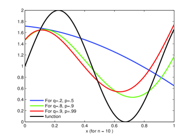
Figure 1:

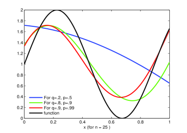
Figure 2:

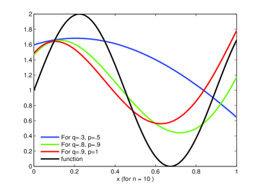
Figure 3:

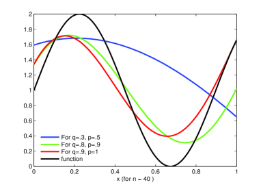
Figure 4: